Negative Diffusivity of Shorelines via the Littoral Drift Rose Concept ^†

Abstract

Conventionally, long-term coastline evolution is usually described using the diffusion equation. Particularly, the diffusion coefficient, ε, is a function of the wave angle: this implies that the diffusivity can assume negative values when wave angles are >45°. The negative-diffusivity concept is often unfamiliar to engineers; therefore, the main purpose of this study is to further investigate its possible implications on shoreline evolution. Practically, negative diffusivity leads to the instability of the coast: any existing perturbation indefinitely grows, and periodic fluctuations of the coast (sand waves) are detected. This research will document the presence of unstable behaviors in some areas of the Adriatic coast, corroborated by the concept of Littoral Drift Rose (LDR).

1. Introduction

Recently, a number of research has revealed that the evolution of a coast due to gradients in along-shore sediment transport is highly dependent upon wave angles, triggering an instability in shoreline shape that can generate different types of naturally occurring coastal landforms. Traditional findings showed that on an open, long, sandy coast, long-shore sediment transport tends to smooth the coastline if the angle between wave crests and the shoreline is relatively small [1]. However, for waves approaching at a large angle with respect to the shoreline, the littoral transport gradients, which originate from shoreline irregularities, may reinforce those irregularities, rendering the rectilinear coast unstable. This had been suggested in the past by a number of authors (e.g., [2]), who recognized the potential of this instability mechanism to generate shoreline features at large spatial scales (1–10 km), such as cuspate shorelines, sand waves, and sand spits.

A quantitative investigation of this phenomenon was first presented by [3], and later pursued by [4,5,6]. It was shown that a number of shoreline morphologies around the world were related to this instability [7].

Although these studies showed that high-wave angle instability, and thereby negative diffusion, may be relevant in the formation of coastal undulations and growth, the physics behind the instability was not deeply discussed in the research.

Thus, the aim of the present paper is to provide further insight into the processes behind high-angle wave instability. An analytical modeling of negative diffusivity of the shoreline is presented, and the physics are discussed with the use of very simple concepts based on the LDR approach.

2. Materials and Methods

2.1. The Shoreline Diffusion Theory

The governing equation of the one-line model first introduced by [8] has been simplified by [9] into the diffusion equation, assuming small breaking wave angles and mild shoreline curvature ∂y/∂x. These assumptions allowed for the consideration of a linear relation between wave incidence angle and littoral drift. If the amplitude of the long-shore sand transport rate and the incident breaking wave angle are constant (independent of x and t), transport relation may be combined with the one-line equation to yield:

$$\frac{\partial y}{\partial t}=\epsilon \frac{{\partial }^{2}y}{\partial x^2}$$

(1)

Equation (1) is the “shoreline diffusion equation”, formally identical to the one-dimensional equation describing the conduction of heat in solids. The coefficient ε is interpreted as a diffusion coefficient expressing the time scale of shoreline change following a disturbance. According to existing literature (e.g., [10]), the diffusion coefficient is intensely dependent on breaking wave height, $H_b$, wave direction, ${\alpha }_b$, and the dimensionless empirical coefficient in the sediment transport rate formula, K [11].

Ref. [10] proposed a modeling of the diffusion coefficient of the following form (called the “classical approach”), considering the long-shore transport rate given by the CERC formulation:

$$\epsilon =\frac{K{g}^{0.6}{H}_0^{12/5}{T}^{1/5}}{8\left(s-1\right)\left(1-n\right)2^{1.4}{\pi }^{0.2}{\gamma }^{0.4}}\frac{1}{\left(D_c+D_B\right)}\cos \left(2\left(\beta -{\alpha }_0\right)\right)$$

(2)

In this equation the $\epsilon$ coefficient depends on off-shore wave characteristics. This dependence can lead the diffusion coefficient to become negative for wave angles > 45°. Therefore, when the angle between the waves and the shoreline is sufficiently large, small perturbations to a straight shoreline will grow, inducing an unstable behavior of the coast. This can be immediately read in the following section, in which an analytical approach is presented.

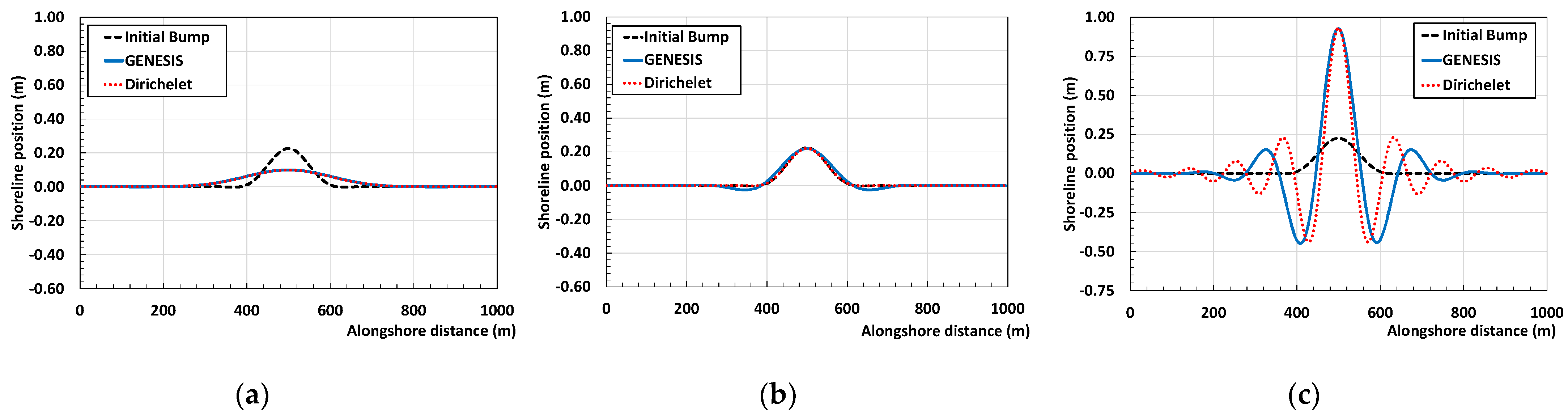
Analytical Modeling of Negative Shoreline Diffusion

The case of a coast with a length of $l$, with an initial position $f\left(x\right)$, is analyzed here. The domain is bound by two pinned points, for which shoreline position $y\left(x,t\right)$ does not move over time. This implies no interruption on the long-shore sediment transport, and the alongshore littoral gradient constant over time.

Mathematically, the pinned boundary conditions for the problem analyzed here give rise to a Dirichlet problem, with Equation (1) as the governing equation, $y\left(x,0\right)=f\left(x\right)$, the initial condition and $y\left(0,t\right)=0 , y\left(l,t\right)=0$ the conditions on the bounds domain.

The Dirichlet problem can be solved by applying the separation of variable technique, for which the general solution can be written as:

$$y\left(x,t\right)={\displaystyle \sum }_{n=1}^{\infty }{A}_{0n}{e}^{-{\left(\frac{n\pi }{l}\right)}^2\epsilon t}\mathrm{sen}\left(\frac{n\pi }{l}x\right)$$

(3)

With:

$$A_{0n}=\frac{2}{l}\underset{0}{\overset{l}{{\displaystyle \int }}}f\left(x\right)\mathrm{sen}\left(\frac{n\pi }{l}x\right)dx$$

(4)

In Equation (3) the time function is an exponential function, in which it compares the diffusion coefficient $\epsilon$. The shoreline response strictly obeys the sign of the coefficient. If the diffusion coefficient is considered positive, the response of the shoreline to an external perturbation of the system is to diminish any protuberance of the initial shoreline position. A positive sign of diffusion occurs when in stable conditions, in other words when the wave angle is less than 45°; otherwise, with wave angle > 45°, $\epsilon$ becomes negative and unstable conditions occur. In fact, by representing the initial condition $f\left(x\right)$in terms of a sine Fourier series, we see the initial shoreline is made up of a series of n components characterized by a certain frequency, of which, small bumps or holes will be characterized by lower frequencies. When entering Equation (3) with a negative diffusion, the response is to enhance the lower frequencies of the shore, therefore, bumps will accrete and holes erode. This effectively resembles what happens in an unstable shoreline condition.

This is proved by considering a straight coastline of 1 km length, initially perturbed by a small bump of 20 cm (Figure 1a–c). The coastline has fixed limits at x = 0 and x = 1000 m. The analytical solution was determined and the shoreline response was analyzed by varying the sign and magnitude of the diffusion coefficient. Moreover, the analytical solution was compared with the corresponding numerical modeling carried out with GENESIS [12], in which the change in sign and magnitude of the shoreline diffusivity is obtained by varying the off-shore wave angle (from 0° to 80°).

As seen in Figure 1, with the increase of the off-shore wave angle, which ranges from 0 to 80°, the initial bump tends to grow when arriving at high wave angle (>45°). Particularly, the numerical solution fits properly with the analytical one, confirming the absolute power of the simple one-line theory to predict shoreline evolution.

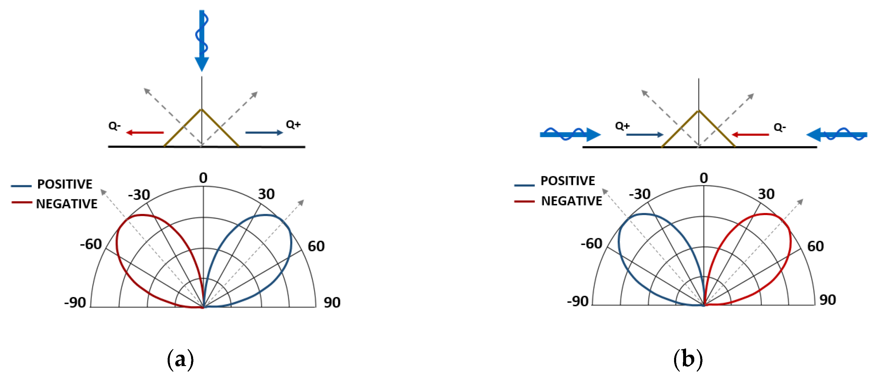
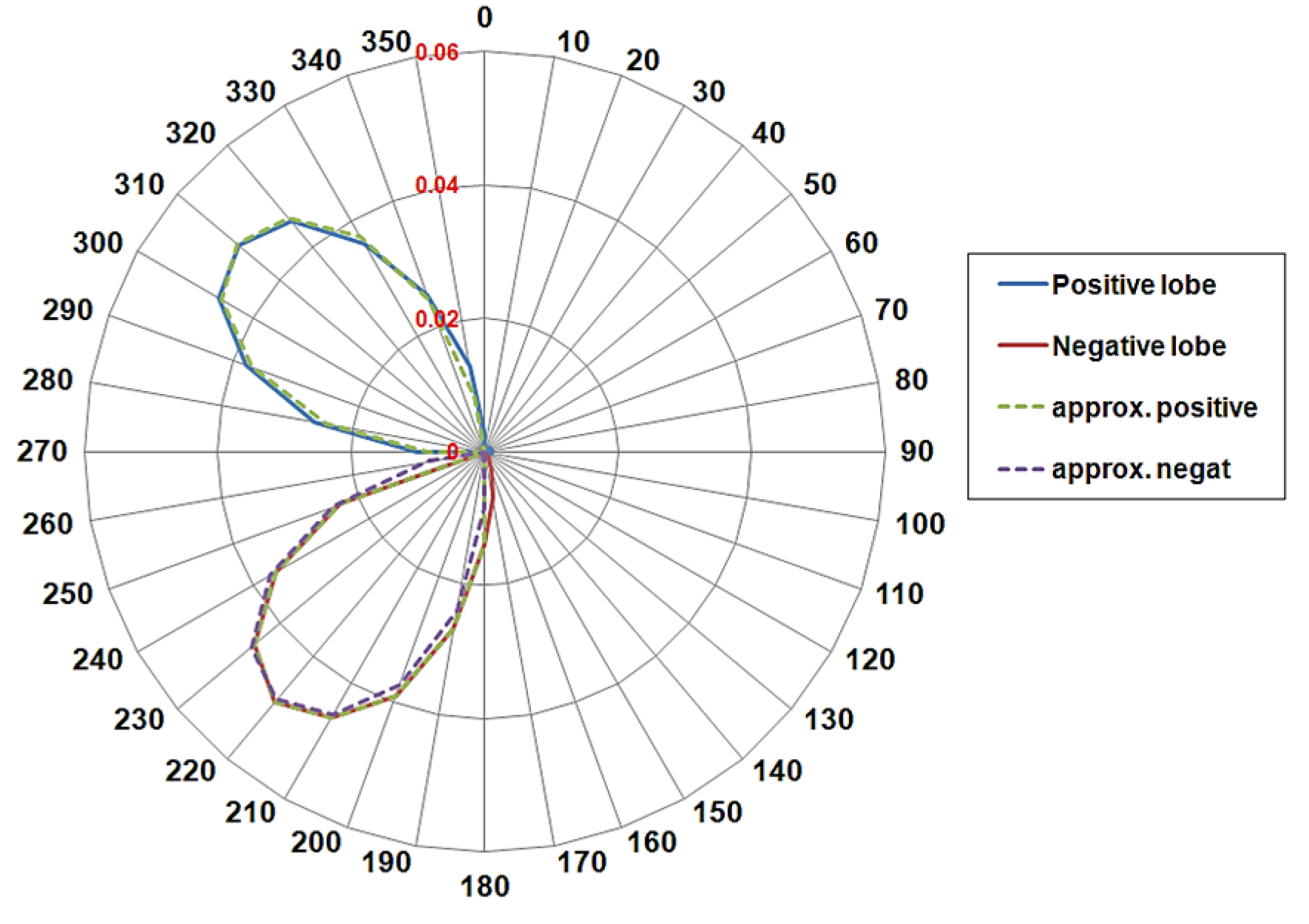
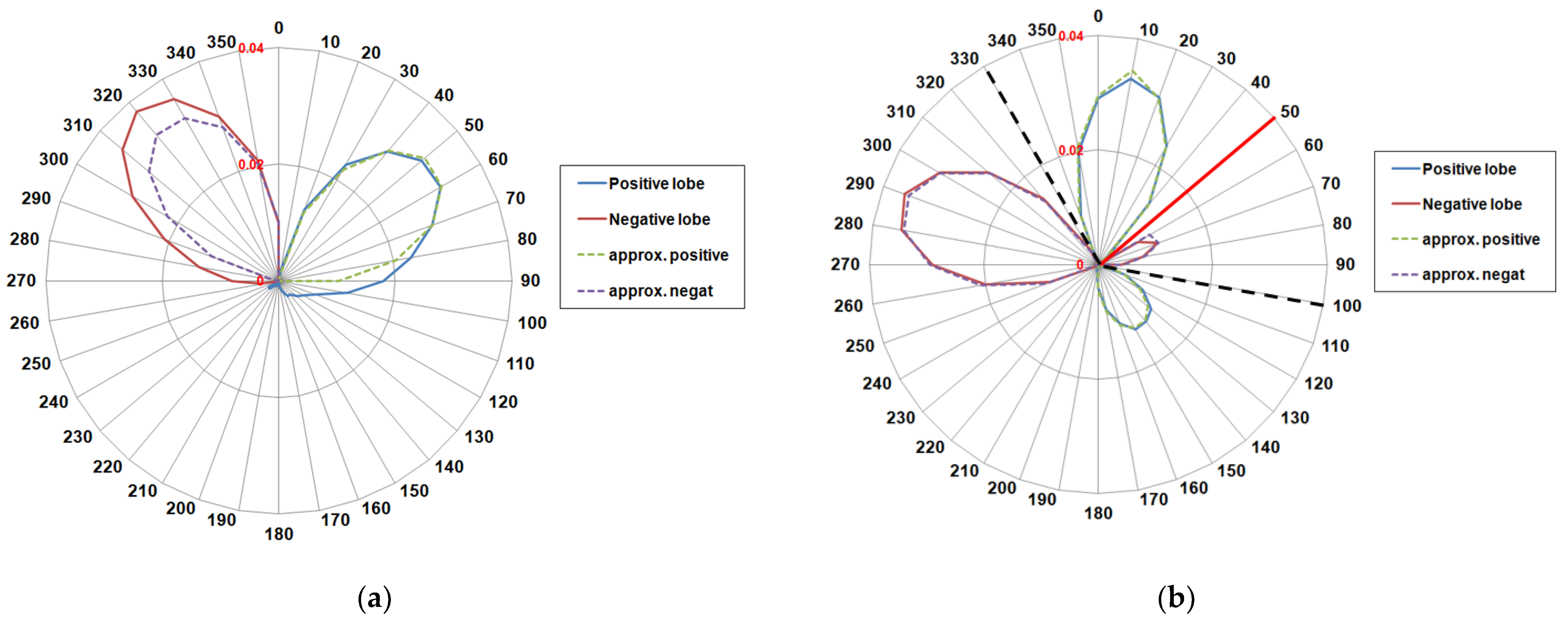
2.2. LDR Concept to Detect Possible Instabilities of Shoreline

Ref. [2] first introduced the littoral drift rose (LDR) concept, where littoral transport is represented in a polar graph by varying the shoreline orientations, (the wave climate to be uniform over the coastal area).

Therefore, the net potential littoral drift rate, (β), for a stretch of coast with normal azimuth β, can be calculated as follows:

$$Q\left(\beta \right)={{\displaystyle \sum }}_{{\alpha }_{0i}=\beta -\raisebox{1ex}{$\pi $}\!\left/ \!\raisebox{-1ex}{$2$}\right.}^{{\alpha }_{0i}=\beta +\raisebox{1ex}{$\pi $}\!\left/ \!\raisebox{-1ex}{$2$}\right.}{p}_i\frac{K·{\left(H_{s0,i}\right)}^{2.4}·{\left(T_{p0,i}\right)}^{0.2}·g^{0.6}}{16·\left(s-1\right)·\left(1-n\right)·{\pi }^{0.2}·{\gamma }^{0.4}·2^{1.4}} sin\left[2\left(\beta -{\alpha }_{0i}\right)\right]$$

(5)

where, $H_{s0,i}$, $T_{p0,i},$ ${\alpha }_{0i}$are the wave parameters of components wave climate is made up of, while $p_i$ is the probability of occurrence; $K$ is a sediment transport coefficient estimated empirically, $g$ is gravity, $s$ = 2.6 is the ratio between the specific gravity of sediment and that of water, $n$ = 0.4 is the in-place porosity, and $\gamma$ = 0.6 is the breaker index (wave height to depth ratio). Given a time-averaging interval, the total positive and negative littoral transports are calculated and plotted in a polar graph, which generally exhibits a null-point, that is the shoreline orientation at which littoral transport nullifies (positive and negative drifts have the same magnitude).

Following the approach by [2], the effect of the whole wave climate in terms of littoral transport is found to be equivalent to that which would occur for a single wave component, of parameters H_s0,eq, T_p0,eq, α_0,eq:

$$Q\left(\beta \right)={{\displaystyle \sum }}_{{\alpha }_{0i}=\beta -\raisebox{1ex}{$\pi $}\!\left/ \!\raisebox{-1ex}{$2$}\right.}^{{\alpha }_{0i}=\beta +\raisebox{1ex}{$\pi $}\!\left/ \!\raisebox{-1ex}{$2$}\right.}{p}_i·\frac{K·{\left(H_{s0,i}\right)}^{2.4}·{\left(T_{p0,i}\right)}^{0.2}·g^{0.6}}{16·\left(s-1\right)·\left(1-n\right)·{\pi }^{0.2}·{\gamma }^{0.4}·2^{1.4}} sin\left[2\left(\beta -{\alpha }_{0i}\right)\right]\cong G_{eq}· sin\left[2\left(\beta -{\alpha }_{0,eq}\right)\right]$$

(6)

where:

$$G_{eq}=\frac{K·{\left(H_{s0,i}\right)}^{2.4}·{\left(T_{p0,i}\right)}^{0.2}·g^{0.6}}{16·\left(s-1\right)·\left(1-n\right)·{\pi }^{0.2}·{\gamma }^{0.4}·2^{1.4}}$$

(7)

Consequently, the “Total-LDR”, relative to the whole climate, can be condensed into a form that is representative of a single wave propagating from a single direction (“Equivalent-LDR”). The equivalent wave direction α_0,eq corresponds to the LDR node, while wave height and period can be inferred from Equation (7).

As discussed in [2,10], the LDR concept can be successfully used to assess if shoreline behavior should be of a stable or an unstable type. In the scenario where one predominant directional mode occurs orthogonal to the general shoreline orientation, the resulting LDR is of a stable type, showing the positive drift lobe to the right of the negative one (Figure 2a). Under this condition, typically observed in open coast areas where longer fetches lie normal to the shoreline, any natural or man-made perturbations of the coast is diminished over time.

By contrast, when longer fetches exist more parallel to the shore while shorter ones exist perpendicular to the shore, an unstable LDR occurs, in which the negative (net) drift lobe lies to the right of the positive (net) one. Figure 2b shows an extreme example of an unstable shoreline scenario where the wave climate consists of two equal but opposite wave components parallel to the general shoreline orientation. For this scenario, a perturbation in the shoreline (however initiated) is unstable, and grows (i.e., see [2]).

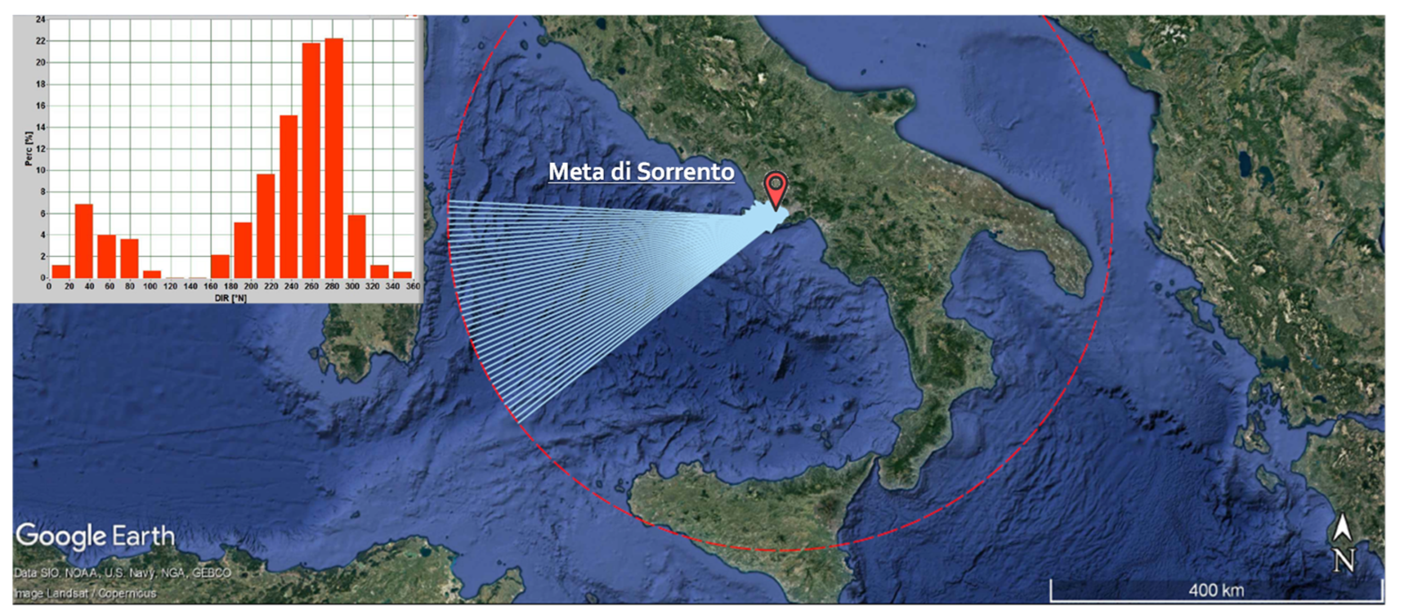
2.3. Comparing Different LDRs of the Italian Seas

The unstable conditions found by Walton and Dean, and recently further analyzed by [6,7] can also be detected in the Italian seas, particularly in the Adriatic Sea, which presents the same characteristics of the elongated water bodies analyzed in previous literature.

According to the LDR approach, the birth of unstable conditions on a certain stretch of coast, and consequently the formation of unstable plane shapes, will be clear in the light of the null-type of the LDR graph. Therefore, for the case of the Adriatic Sea, an unstable LDR is expected. However, as it will be shown in the next sections, although unstable wave components are not able to generate an unstable LDR for the Adriatic Sea, their presence determines a change in the LDR shape. Two different types of LDRs are presented and compared in the following sections.

2.3.1. The LDR Graph for the Tyrrhenian Sea

A stable LDR condition can be detected at the coastal site of Meta di Sorrento, which faces the Tyrrhenian Sea. As shown in Figure 3, for this case, longer fetches lie quite normal of the shore; consequently, the predominant mode of wave climate is near orthogonal to the general shoreline orientation. As a consequence, the wave climate is of a monomodal type: in this case, the most frequent direction originates from a single direction which is responsible of the long-term sculpting of the coast (Figure 3).

Figure 4 shows the resulting LDR graph: in this case, as expected, the stable type is determined, and the graph shows nearly symmetrical lobes with the positive (net) littoral drift to the right to the negative (net) one. The equivalent wave component, calculated from the procedure suggested by [10], has a wave height of about 1 m and an equivalent direction, corresponding to the null point of the total LDR, equal to 265° N.

Most notably, Figure 4 shows that the equivalent component is able to accurately fit the total LDR, since the average net drift rose for the total wave climate has lobes that cause the magnitude to vary in a sinusoidal manner. Particularly, from Figure 4 it is seen that the total LDR do not exhibit asymmetrical lobes: the net drift varies over the shoreline normally, in a sinusoidal manner, and so the equivalent climate is able to accurately fit the transport due to the entire wave climate.

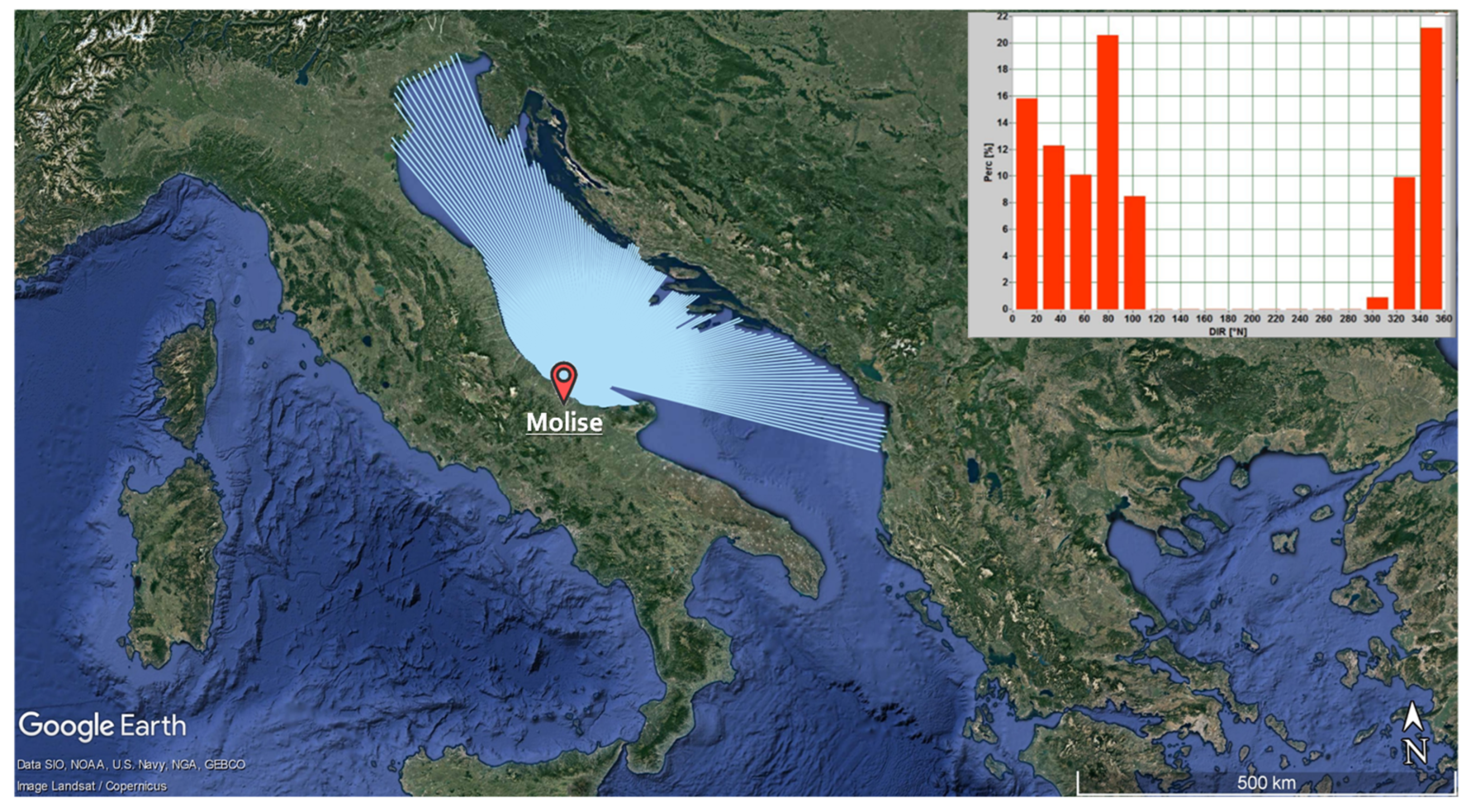
2.3.2. The LDR Graph for the Adriatic Sea

Conversely, if we move to the Adriatic Sea, matters look quite different. Focusing on the Molise case study, presented in the previous chapter, we can see long fetch lengths for wave growth more parallel to the shore, while short fetch lengths perpendicular to the shore (Figure 5). As a result, wave climate is affected by an inherent bimodality, with two opposite modes, from 340° N and 80° N respectively (Figure 5).

Surprisingly, the net littoral transport here results in a stable LDR (Figure 6a). As shown, this LDR graph, different to the Meta di Sorrento case study, exhibits nearly asymmetrical lobes.

The shape of the LDR graph suggests that the magnitude of littoral transport does not vary in a sinusoidal manner, and the approximation given by the single equivalent sinusoidal wave component is not more satisfactory. In this case, the equivalent component gives a proper approximation only for the positive lobe, while an underestimation of the negative lobe is detected. This happens because longer fetches lie more oblique to the shore, which generate high angle components, which then generate a possible unstable condition. Therefore, we considered a wave climate only made up of the more oblique direction, generated by fetches comprised between 320 and 339° N from the northern quadrant and between 93 and 104° N from the east quadrant. The resulting LDR graph is then determined using two opposite wave components, with different magnitudes, from 330° N and 100° N respectively (Figure 6b). These two components lead, within the shoreline orientation range of Molise coast (340° N–110° N), to an unstable LDR. The equivalent “unstable” wave component is oriented toward 50° N, (the red line in Figure 6b). The unstable component detected from the graph can cause, in turn, a negative diffusion zone within coastal stretches nearly orientated towards 50° N.

3. Results and Conclusions

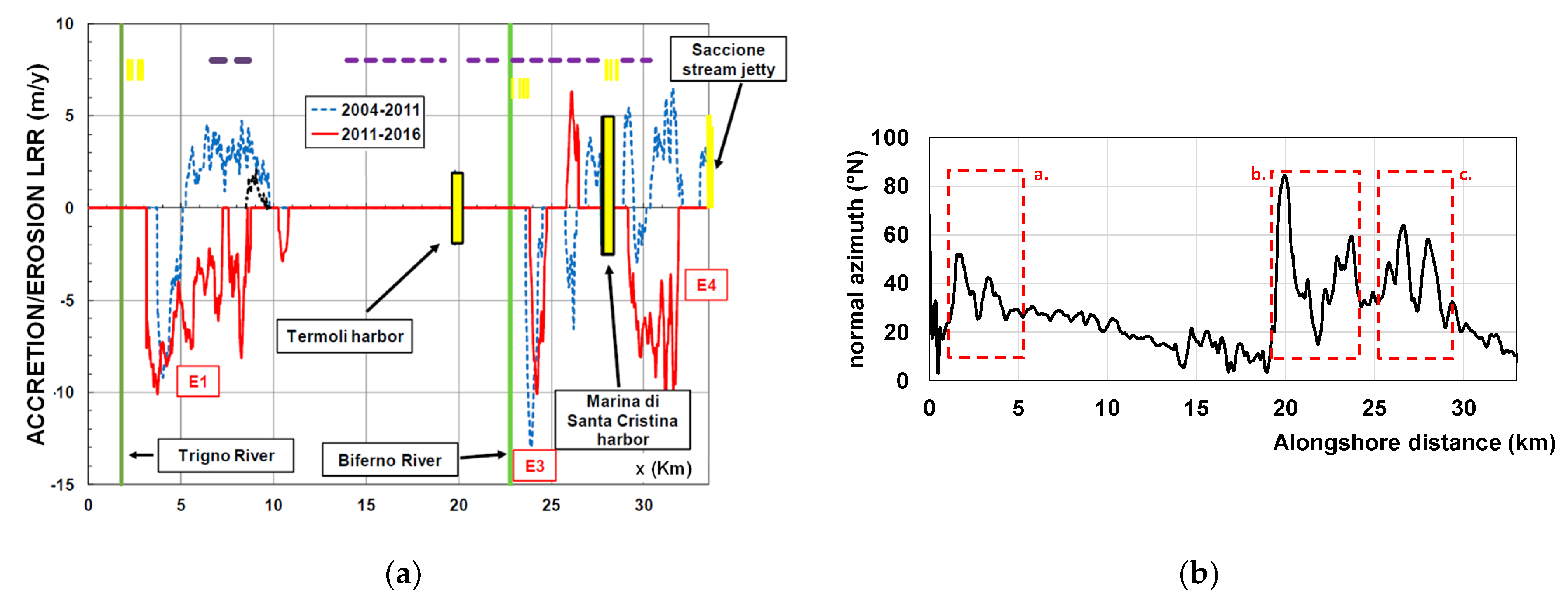
The Inspection of Shoreline Instabilities on the Molise Coast

In the framework of a collaboration between the University of Molise and the University of Napoli “Federico II”, a shoreline change study was carried out in order to analyze the most recent trends of Molise coast evolution, and investigate the possible relationships between wave direction and shoreline response [13,14]. More recently, [15,16,17] analyzed the average rate of shoreline change of the entire Molise coast within the reference time interval 2004–2016, using the Linear Regression Rate (LRR) as an indicator. Those analyses led us to propose that the unstable components, generated by longer fetches, are responsible for particular aspects of shoreline evolution.

Ref. [15] demonstrates that the stable component is sufficient to explain the bulk of the Molise coastline evolution; additionally, the detailed analysis presented by [18], for the Trigno river mouth area verified this. A more accurate analysis revealed that, recently, the erosion processes widely accelerated, suddenly spreading to the neighboring areas of the foremost erosion zones. These latest dynamics are depicted in Figure 7a, where the LRR function has been determined by splitting the analysis time window into two parts, from 2004 to 2011 and from 2014 to 2016, respectively. It shows that accretionary bulges preceded erosional depressions in the area just south the river mouths (Trigno and Biferno respectively), and also for the area just south the Marina of Santa Cristina harbor. Particularly, as shown in Figure 7b, the aforementioned areas affected by these instability features have shoreline orientations about 30–40° N, very close to the unstable orientation of 50° N detected from the LDR in Figure 6b.

This peculiar evolution of the Molise coast can be ascribed to the presence of accretion/erosion sand waves, which follow one another along the shore in the direction of the net littoral drift. These local irregularities of the beach form, appreciable by comparison of beach profiles with time and distance along the beach, can be associated with the negative diffusivity generated by unstable wave components, with a high angle with respect to the shoreline average. Particularly, according to the analysis of [6], sand waves occur for climates with a slight predomination for high-angle waves and a moderate amount of directional asymmetry, which is just the case of the directional distribution of the Molise wave climate.

References

1. Komar, P.D. Beach Processes and Sedimentation, 2nd ed.; Prentice Hall: Upper Saddle River, NJ, USA, 1998. [Google Scholar]
2. Walton, T.L.; Dean, R.J. Application of Littoral Drift Roses to Coastal Engineering Problems. In Proceedings of the Conference on Engineering Dynamics in the Surf Zone, Institution of Engineers, Sydney, Australia, 14–17 May 1973; pp. 221–227. [Google Scholar]
3. Ashton, A.; Murray, A.B.; Arnoult, O. Formation of coastline features by large-scale instabilities induced by high-angle waves. Nature 2001, 414, 296–300. [Google Scholar] [CrossRef] [PubMed]
4. Falques, A. On the diffusivity in coastline dynamics. Geophys. Res. Lett. 2003, 30, 2119. [Google Scholar] [CrossRef]
5. Falques, A.; Calvete, D. Large-scale dynamics of sandy coastlines: Diffusivity and instability. J. Geophys. Res. Earth Surf. 2005, 110, C03007. [Google Scholar] [CrossRef] [Green Version]
6. Ashton, A.D.; Murray, A.B. High-angle wave instability and emergent shoreline shapes: 1. Modeling of sand waves, flying spits, and capes. J. Geophys. Res. Earth Surf. 2006, 111, F04011. [Google Scholar] [CrossRef] [Green Version]
7. Ashton, A.D.; Murray, A.B. High-angle wave instability and emergent shoreline shapes: 2. Wave climate analysis and comparisons to nature. J. Geophys. Res. Earth Surf. 2006, 111, F04012. [Google Scholar] [CrossRef] [Green Version]
8. Pelnard-Considere, R. Essai de theorie de l’evolution des formes de rivage en plages de sable et de galets. In 4th Journees de l’Hydraulique, Les Energies de la Mer, III; La Houille Blanche: Grenoble, France, 1956. [Google Scholar]
9. Larson, M.; Hanson, H.; Kraus, N.C. Analytical Solutions of the One-Line Model of Shoreline Change; Technical Report CERC-87; U.S. Army of Engineer Waterways Experiment Station, Coastal Engineering Research Center: Washington, DC, USA, 1987. [Google Scholar]
10. Walton, T.L.; Dean, R.J. Longshore Sediment Transport Via Littoral Drift Rose. Ocean Eng. 2010, 37, 228–235. [Google Scholar] [CrossRef]
11. US Army Corps of Engineers. Shore Protection Manual; Coastal Engineering Research Centre: Washington, DC, USA, 1984.
12. Hanson, H. GENESIS: A Generalized Shoreline Change Numerical Model for Engineering Use. Ph.D. Thesis, University of Lund, Lund, Sweden, 1989. [Google Scholar]
13. Rosskopf, C.M.; Di Paola, G.; Atkinson, D.E.; Rodriguez, G.; Walker, I.J. Recent shoreline evolution and beach erosion along the central Adriatic coast of Italy: The case of Molise region. J. Coast. Conserv. 2018, 22, 879–895. [Google Scholar] [CrossRef]
14. De Vincenzo, A.; Covelli, C.; Molino, A.J.; Pannone, M.; Ciccaglione, M.C.; Molino, B. Long-term Management Policies of Reservoirs: Possible Re-use of Dredged Sediments for Coastal Nourishment. Water 2019, 11, 15. [Google Scholar] [CrossRef] [Green Version]
15. Buccino, M.; Di Paola, G.; Ciccaglione, M.C.; Rosskopf, C.M. A Medium-Term Study of Molise Coast Evolution Based on the One-Line Equation and “Equivalent Wave” Concept. Water 2020, 12, 2831. [Google Scholar] [CrossRef]
16. Di Paola, G.; Ciccaglione, M.C.; Buccino, M.; Rosskopf, C.M. Influence of Hard Defence Structures on Shoreline Erosion Along Molise Coast (Southern Italy): A Preliminary Investigation. Rendiconti Online Soc. Geol. Ital. 2020, 52, 2–11. [Google Scholar] [CrossRef]
17. Buccino, M.; Ciccaglione, M.C.; Di Paola, G. The use of one-line model and littoral drift rose concept in predicting long term evolution of the Molise coast. In Proceedings of the 30th International Ocean and Polar Engineering Conference, Virtual, 11–16 October 2020. [Google Scholar] [CrossRef]
18. Ciccaglione, M.C.; Buccino, M.; Di Paola, G.; Calabrese, M. Trigno River Mouth Evolution Via Littoral Drift Rose. Water 2021, 13, 2995. [Google Scholar] [CrossRef]
Figure 1. Numerical (orange solid line) and analytical (black dot line) comparison of the evolution of an initial bump under different wave conditions. (a) 10° (b) 50° (c) 80°.
Environsciproc 21 00078 g001
Figure 2. (a) Stable littoral drift rose. Note blue line (positive drift) lobe of LDR is on the right side of diagram. (b) Unstable littoral drift rose. Note blue line (positive drift) lobe of LDR is on the left side of diagram.
Environsciproc 21 00078 g002
Figure 3. Fetches of Meta di Sorrento site, which faces the Tyrrhenian Sea. The upper panel shows the frequency direction wave climate.
Environsciproc 21 00078 g003
Figure 4. Littoral Drift Rose of Meta di Sorrento. Solid lines represent the Total LDR (blue line positive drift, red line negative drift), while dashed lines represent the Equivalent rose, given by a sinusoidal component of parameters: H0,eq = 1 m, Tp,eq = 5 s, α0,eq = 265° N.
Environsciproc 21 00078 g004
Figure 5. Fetches of Molise coast site which faces the Adriatic Sea. The upper panel shows the frequency direction wave climate.
Environsciproc 21 00078 g005
Figure 6. (a) Littoral Drift Rose of Molise coast. Solid lines represent the Total LDR (blue line positive drift, red line negative drift), while dashed lines represent the Equivalent rose, given by a sinusoidal component of parameters: H0,eq = 0.83 m, Tp,eq = 5.08 s, α0,eq = 9° N. (b) Littoral Drift Rose of Molise coast computed from the more oblique directions (320–339° N and 93–104° N). Dashed lines represent the Equivalent rose, given by two equivalent component of parameters: H0,eq = 0.91 m, Tp,eq = 5.08 s, α0,eq = 330° N and H0,eq = 0.56 m, Tp,eq = 5.08 s, α0,eq = 110° N. The red solid line represent the direction of the unstable component, which generates within the normal range of Molise coast (340–120° N).
Environsciproc 21 00078 g006
Figure 7. (a) LRR of Molise coast. Horizontal dashes indicate detached breakwaters; vertical dashes indicate groin fields. Red line 2014–2016; blue dashed line 2004–2011. (b) normal azimuth along the Molise coast. Area a. Trigno river mouth area, area b. Biferno river mouth area, area c. Santa Cristina Harbor area.
Environsciproc 21 00078 g007
Publisher’s Note: MDPI stays neutral with regard to jurisdictional claims in published maps and institutional affiliations.