Abstract
In this paper, two different strategies are presented that allow for the assessment of the effects of climate change on urban pluvial flooding, in order to understand potentialities and limitations, advantages and drawbacks. The two strategies are hereby defined as “top-down” and “bottom-up”, according to the relative position of climate change modelling with respect to flood modelling (upstream for top-down, downstream for bottom-up). To provide a practical example, the two strategies are applied to a case study located in Naples, Italy. However, they can be successfully extended for the assessment of any potential impact of climate change in any location.
1. Introduction
According to the most recent Reports of the Intergovernmental Panel on Climate Change (IPCC), climate change is very likely to result in extreme rainfall regime all over the world [1]. The perils induced by a possible increase in the severity of extreme rainfall events are expected to be particularly critical in urban areas, because of the high exposures (people, buildings, infrastructure, economic activities) and because urban areas are usually subject to rainfall-related risks already under current climate conditions [2]. This particularly applies to historical urban settlements that have experienced continuous population growth, resulting in complex and stratified urban drainage systems that have often been developed under the structural constraints posed by historical buildings and underground ruins.
A robust and reliable quantification of climate change effects on the extreme rainfall regime of urban areas, and the related impacts in terms of urban flooding, is a scientific and technical challenge, especially when the interest concerns future climate scenarios, as per the guidelines of IPCC reports. The currently available rainfall projections, as those included in the EURO-CORDEX initiative (https://www.euro-cordex.net/, accessed on 1 September 2018, [3]), come from the running of Regional Climate Models (RCMs) that are not able to fully resolve atmospheric convection (which is an acknowledged cause for hazardous extreme rainfall events) but only treat it as a “sub-grid” process by means of specific parameterizations [4,5]. As a result, projection data usually have to undergo a bias adjustment post-process to be used as a suitable input for impact models, such as flood modelling [6]. This adds a significant computational burden to the process, alongside the need to consider multiple climate scenarios (namely, RCPs), multiple future horizons (namely, short-term and long-term), and multiple climate models.
In order to deal with such uncertainties, simplified approaches for flood modelling are particularly appreciated because they do not add computational burden to the simulation chain [7]. However, simplifications are only suitable when the overall goal of the analysis is to look at some macroscopic features of flooding, for example when the objective is a comparison among different alternatives (such as different intervention scenarios, or different rainfall severity levels): this is usually referred to as “scenario analysis” [8,9]. In turn, detailed flood models are needed when the focus is on specific locations or when spatialized features have to be investigated, such as the distribution of flood depths over the domain.
In this paper, two opposed strategies allowing for the quantification of climate change effects on urban flooding are compared and discussed. As will be clarified in the Methods Section, the first strategy can be defined as “top-down”: it consists of a fully detailed urban pluvial flood model where climate change acts by altering the rainfall. The second can be defined as “bottom-up” since flood modelling is performed with the same degree of detail but the climate change information is only included afterwards, when the flood modelling has already been performed. The Case Study Section describes the pilot area and the rainfall data used as inputs. The Results Section shows the products of the two approaches and the Discussion Section highlights potentialities and drawbacks.
2. Methods
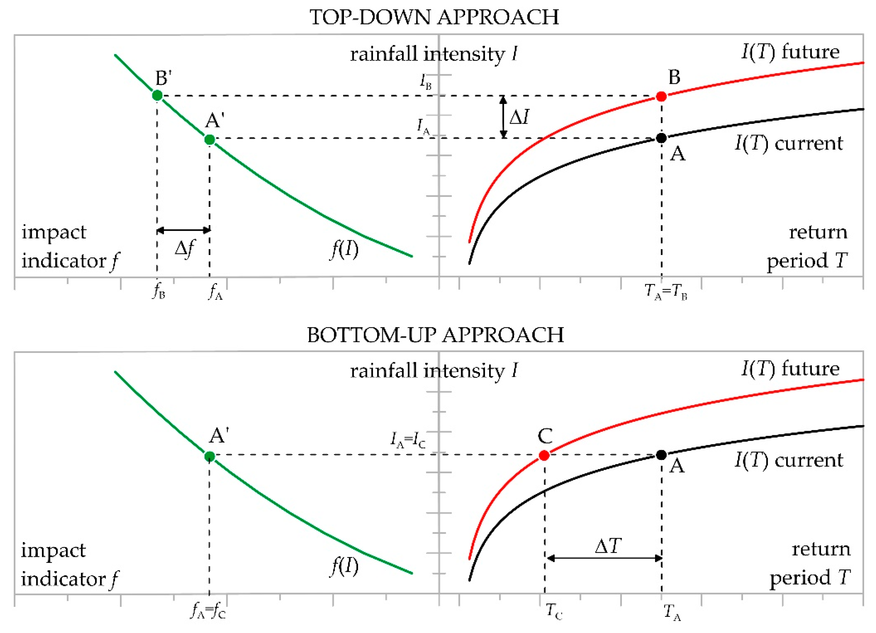
Figure 1 shows the difference between the “bottom-up” strategy, proposed by [7] and a more common “top-down” approach [10,11].
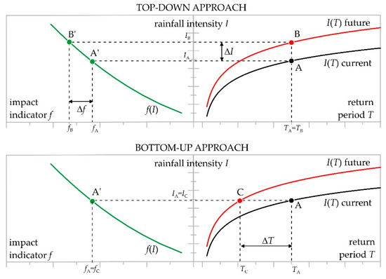
Figure 1.
Impact simulation chain with a top-down (upper panel) and a bottom-up (lower panel) approach.
Let point A with coordinates (TA, IA) represent a rainfall event with a selected duration that, under current (observed) climate conditions, has an intensity IA and occurs with an average frequency of TA years. Let point A′ with coordinates (fA, IA) represent the flood conditions over a domain of interest for the rainfall event A. According to such a notation, f can be any desired flood feature of interest, such as flooded area, runoff volume, flood depth in a specific location, hazard level in a portion of the domain, etc.: in other words, the “impact” of rainfall on the domain.
Under current climate conditions, the relationship between T and I is usually known, either by means of extreme value analysis of observed site data or by means of a regional frequency analysis, which is the case in Italy (http://www.idrologia.polito.it/gndci/Vapi.htm, accessed on 1 September 2018). The relationship between I and f is not known a priori but it can be built by running the flood model for a sufficient number of rainfall scenarios.
Under future climate conditions, a new relationship can be built between T and I so that, for the very same return period TB = TA, a new intensity value IB can be found (point B), with IB > IA, implying an increase in the severity of the extreme rainfall regime because of climate change. A new impact value fB will occur (point B′), with fB > fA if IB > IA, and vice versa. The increase ∆f is the focus of the top-down approach.
Let point C identify a rainfall event with the very same intensity and impact values of A (IC = IA and fC = fA). However, as shown by Figure 1, point C occurs with a novel return period TC, with TC < TA if climate change entails an increase in the severity of extreme rainfall. The reduction ∆T is the focus of the bottom-up approach.
3. Case Study: Pilot Area, Rainfall Scenarios and Modelling Assumptions
3.1. Pilot Area
The domain used for the analysis is Fuorigrotta, one of the administrative units of the City of Naples, located in the western part of the city. The overall domain is about 2.1 km2 wide and it roughly coincides with the storm water drainage catchment serving the neighborhood. The area comprises a highly strategic area (the football stadium and the commercial activities nearby) and a residential area, where the secondary road network often experiences traffic jams during rainfall events, both because of the possible limited visibility and because of frequent potholes. Additional information about the pilot area can be retrieved in [11].
3.2. Flood Modelling Assumptions, Tools and Indicators
CADDIES Caflood is a flood modelling software relying on Cellular Automata (CA), and based on a square regular grid and von Neumann neighborhood [12]. This model employs simple transition rules and a weight-based system rather than shallow water equations to resolve the flow movement, minimizing the need for solving computationally expensive algorithms while maintaining high accuracy [9]. Caflood is able to account for spatially and temporally variant rainfall intensities and infiltration rates, which must be manually fed by users as time series; the main outputs consist of spatially and temporally distributed water depths and flow velocities. In this work the focus is on the flooded area indicator (FAI), defined as the total extent of flood, expressed as a percentage of the flood-prone area of the domain. Since FAI varies over time during the flood event, the peak value is considered: peak “p” refers to an ideal condition where each cell of the domain experiences its maximum flood depth.
All the details about the flood modelling component, including the parameters’ values for infiltration and roughness, and the role of the sewer network, are explained in [11]. Details are not given here, since the approach, which is the focus of this work, holds regardless of the domain and the conceptual/technical modelling in use.
3.3. Rainfall Scenarios
The National Flood Evaluation Project (“VAPI”) developed a regional rainfall frequency analysis [13] for Italy that relies on the storm index method [14]. According to the storm index method, the annual maximum extreme rainfall depth (h) for any rainfall duration (tr) and return period (T) can be computed as the product of the average of annual maxima μ[h(tr,T)] and a growth factor kT:
The former represents the deterministic part of the extreme rainfall regime, and can be computed as a parametric function of rainfall duration and site elevation. The latter represents the probabilistic part, and can be computed relying on the Two-Component Extreme Value distribution, although a simplified logarithm dependence on the return period is also available. For the area of interest, parameters’ values for both terms are provided by the VAPI Synthesis Report for the Campania Region [13], so that the relationship between T and h is known under current climate conditions. For a rainfall duration of one hour and an elevation averaged within the domain (equal to 46 m above sea level), the relationship is the following:
where μ = 27 mm, a = 0.384, and b = 0.614, and h is expressed in mm. In [15], a novel bias adjustment technique relying on Quantile Delta Mapping [16] was applied to 19 climate projections of the EURO-CORDEX ensemble, for the future horizon 2071–2100 under RCP 4.5 and 8.5. According to this approach, the rainfall depth for any given rainfall duration and return period, expected in a future climate scenario, is provided by the product of the rainfall depth for the same duration and return period occurring in the observed climate, and a change factor CF which can be expressed as a logarithm function of return period T (Equation (3)). Finally, for a rainfall duration of one hour, the future, bias-corrected rainfall depth (hbc) can be expressed by combining Equations (2) and (3), obtaining Equation (4):
Table 1 shows the list of coefficients (c and d) for a small selection of the 19 tested and bias-corrected climate simulation chains (CSCs, comprised of a driving global model and a RCM): specifically, only models identified by labels #9, #11, #12, and #19 are retained, since they provide a good representation of the overall spread of the ensemble. It can be noted from Table 1 that c = 0 for all the models and RCPs. This occurs because, for such models, the change factor (CF) is only due to a shift in the average of annual maxima, whereas the shape of the probabilistic distribution of annual maxima remains unchanged [15]. It can also be observed from Table 1 that for model #11 the RCP 8.5 scenario provides a decrease in the severity of extreme rainfall (in opposition with the other considered models) testified by the lower value of d under RCP 8.5 with respect to RCP 4.5.

Table 1.
Parameters of Equation (3) for a selection of Climate Simulation Chains.
Flood simulations were performed using rainfall intensity values referring to a duration of 1 hr as the input. For the top-down strategy, two input rainfall scenarios were used, both occurring under current climate conditions, with return periods T1 = 10 yr and T2 = 200 yr. For each of them, updated rainfall values for each CSC and each RCP were derived by Equation (4) with parameters in Table 1: they provided 2 × 4 = 8 additional flood simulations, for a total of ten. For the bottom-up strategy, six input rainfall scenarios were used that occurred, under current climate conditions, with return periods of 10, 20, 30, 125, 200, and 250 years.
4. Results
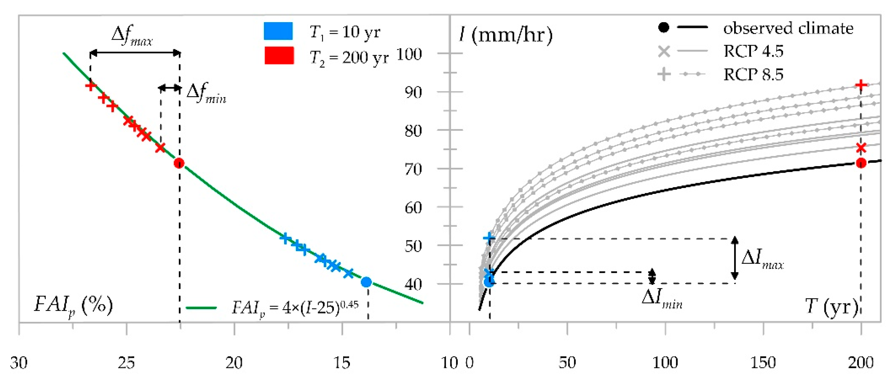
Figure 2 shows the application of the top-down approach for two reference return periods (T1 = 10 yr and T2 = 200 yr). For each return period, first the rainfall intensity values corresponding to current and future climate are identified by means of Equations (2) and (4). Then, each so-determined rainfall scenario is set as the input for CADDIES Caflood and a value of the impact indicator is extracted. In this work, impact results are shown in terms of the lumped flood indicator FAIp. The experimental points in the plane (I, FAIp) gather along a common curve whose equation is shown in Figure 2.
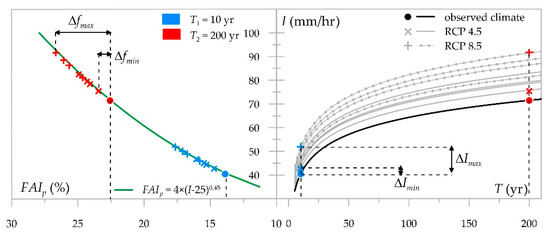
Figure 2.
Impact simulation chain with a top-down approach: (left) flood modelling; (right) climate change modelling. Fitting green line in the left panel has R2 > 99%. Grey curves in the right panel represent the CSCs in Table 1 (from top to bottom under both RCPs: #12, #19, #9, #11). Deltas are visualized for just one experimental point as an example.
For T1, as highlighted in Figure 2, ∆Imin = 5.6% (CSC #19, RCP 4.5) and ∆Imax = 28.3% (CSC #12, RCP 8.5). For T2 the same values hold, since, as testified by Table 1, climate change effects do not vary with the return period (c = 0 for all CSCs). In terms of impact, for T1 ∆fmin = 6.0% and ∆fmax = 27%, whereas for T2 ∆fmin = 3.9% and ∆fmax = 18.1%. All ∆ values are expressed as a percentage increase with respect to current climate conditions. This implies an attenuation of the negative impact of climate change on flooding for increasing severe floods under the current climate conditions. In other words, the higher the severity of flooding under the current climate, the lower the increase in severity because of climate change.
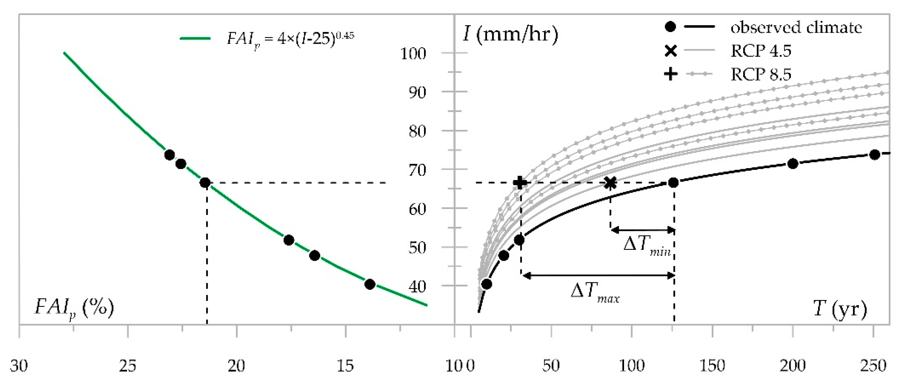
Figure 3 shows the application of the bottom-up approach for six reference return periods (10, 20, 30, 125, 200, 250 yr). For each return period, first the rainfall intensity values corresponding to current climate are identified by means of Equation (2). Then, each so-determined rainfall scenario is set as the input for CADDIES Caflood and a value of the impact indicator is extracted. Then, for each CSC and each RCP scenario, an updated value of the return period is extracted by means of Equation (4). The regression curve FAIp(I) strictly coincides with the curve in Figure 2, but it is derived from different sample points.
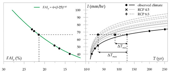
Figure 3.
Impact simulation chain with a bottom-up approach: (left) flood modelling; (right) climate change modelling. The fitting green line in the left panel has R2 > 99%. Grey curves in the right panel represent the CSCs in Table 1 (from top to bottom under both RCPs: #12, #19, #9, #11). Deltas are visualized for just one experimental point as an example.
As suggested by Figure 3, ∆Tmax and ∆Tmin identify a variability range that is significantly small for lower return periods and significantly large for higher return periods. For the smallest T (10 yr), it results in ∆Tmin = −5.0% and ∆Tmax = −67.3%; for the largest T (250 yr), it results ∆Tmin = −33.9% and ∆Tmax = −87.0%.
5. Discussion
In accordance with Figure 1 (specified by Figure 2 and Figure 3), the overall impact modelling can be conceived as comprising of two components, namely the climate change modelling and the flood modelling. Generally speaking, flood modelling and climate change modelling can be performed with any desired detail level according to the scope of the analysis and to the availability of data. In this work, for the top-down strategy, a selection of data from [11] is used that come from the application of CADDIES Caflood, a grid-based tool relying on Cellular Automata. An example of the bottom-up strategy relying on a fully resolved flood model, namely the 2D-SWE model developed by [17], is shown in [7]. For climate change assessments, the envisaged tool should allow for the estimation of updated intensity-duration-frequency (IDF) curves. In this work, the one proposed by [15] is adopted, which is based on Quantile Delta Mapping [16] and on the storm-index method. In [15], results are shown, in terms of Equation (3), for the mean and standard deviation of the ensemble of 19 EURO-CORDEX CSCs. However, in this work, only a selection of 4 CSCs is considered, and the parameters of Equation (3) for these models are presented as a novelty element. Finally, both strategies can be effectively applied for flood impacts other than FAIp.
The two strategies should not be considered strictly as alternatives, but rather as complementary. The first practical difference consists in the different number of simulations that should be performed. For the bottom-up approach, only one flood simulation is required, namely the one referring to current climate, whereas for the top-down approach at least two flood simulations are required, one corresponding to current climate and the other corresponding to a future scenario. In this work, a higher number of simulations is performed to simulate a real-case application: for the top-down approach, only two current climate rainfall scenarios are simulated, and for each of them multiple future scenarios are considered; for the bottom-up approach, six current climate rainfall scenarios are simulated. In the former case, two RCP scenarios are considered, which is usually recommended for climate change studies, and different CSCs (however, an alternative could be considered that uses the mean and a measure of spread for a large ensemble of CSCs). In the latter case, the representation of multiple rainfall percentiles is a common standard in practical applications. The second difference regards the need of assessing climate change effects on extreme rainfall upstream (for the top-down approach) or downstream (for the bottom-up approach) of flood simulations. It should be noted that flood modelling is a common procedure, albeit with different degrees of detail, for practical applications as well as for scientific purposes, and a plethora of codes and tools for flood modelling exist that can be adapted to any situation in terms of data availability and purpose of the analysis [11]. In other words, the reliability of flood modelling is merely a matter of costs, including, in this work, the overall amount of needed resources (data, codes, computational means, personal skills). Instead, climate change modelling is far from being a solved problem, due, for instance, to the availability of suitable CSCs, continuously increasing in terms of resolutions and parameterizations [18]. In other words, the reliability of the climate change modelling component is still an open question, and the related modelling tools should be continuously questioned and/or updated. Keeping this in mind, the bottom-up approach doesn’t entail the need of repeating flood simulations if the function I(T) for future scenarios changes. On the other hand, in the top-down approach, the update of intensity values is performed first, and, if updated intensity changes because of a change in the function I(T) for future scenarios, flood modelling needs to be performed again.
The preferability of the bottom-up against the top-down approach does not hold when it is considered acceptable to infer the values of an impact indicator from the function f(I), instead of extracting it from a flood simulation. This typically occurs for lumped indicators, such as FAIp. In this case, the only restriction on the number of flood simulations is that there should be enough to calibrate the function f(I). However, if flood-related evaluations focus on (i) distributed flood features (e.g., a proper flood mapping), or (ii) on localized indicators (e.g., flood depth at specific coordinates), then the mathematical relationship f(I) becomes (i) useless or (ii) could decrease the reliability of the results. In this case, modelers could rely on one approach over the other according to their needs. For example, if the purpose of the analysis is that of simulating the impacts of specific future rainfall values (e.g., a rainfall value expected in the future with a specific return period, against rainfall values occurring with the same return period in the current climate conditions), then the top-down is the only suitable approach [11]. Instead, if the purpose is that of communicating climate change-related risks, the bottom-up approach is useful since it provides new frequencies for hazardous events that are already perceived as extremes under current climate conditions [7].
6. Conclusions
In this work the advantages, drawbacks, potentialities, and limitations are shown for two different strategies allowing for the estimation of climate change effects on urban flooding. The strategies can be referred to as “top-down” and “bottom-up”, where the labels highlight the position of climate change modelling with respect to flood modelling (upstream or downstream, respectively). The contribution shows results for a pilot area located in Naples, Italy. For this area, IDF curves are updated to include the climate change effects in accordance with the model proposed by [15], and flood modelling is performed by means of CADDIES Caflood [12] and quantified by means of the FAIp indicator [7,11]. However, the entire methodology can be successfully applied with any other climate change or impact modelling tool/metric, and it can also be exported to any other impact different from flooding. For this reason, details about flood modelling are not fully reported in this contribution.
The aim of investigating two different strategies is to help understand which modelling contexts and situations suit each approach best. This contribution shows that the bottom-up approach generally over performs the top-down strategy merely because of the reduced number of requested flood simulations. However, the top-down approach is the only suitable procedure when flood outputs at specific return periods are required. The preferability of one strategy over the other ceases if the impacts can be reliably inferred by a curve f(I), which usually occurs for lumped indicators, such as flooded areas or flood models. If not, then modelers could rely on one approach over the other according to their specific needs.
Author Contributions
Conceptualization and methodology, R.P. and P.C.; software and formal analysis, R.P.; writing—original draft preparation, R.P.; writing—review and editing, P.C., C.C. and G.R.; visualization, R.P.; supervision, P.M. and G.D.G. All authors have read and agreed to the published version of the manuscript.
Funding
This research received no external funding.
Institutional Review Board Statement
Not applicable.
Informed Consent Statement
Not applicable.
Data Availability Statement
Not applicable.
Acknowledgments
The Authors acknowledge the World Climate Research Programme’s Working Group on Regional Climate, and the Working Group on Coupled Modeling, former coordinating body of CORDEX and responsible panel for CMIP5. They also acknowledge the responsible team for CADDIES Caflood at the Centre for Water Systems (University of Exeter) for technical and scientifical support and for providing Pro version. CADDIES Caflood free software and documentation can be found at https://www.cafloodpro.com/caflood-software/ (accessed on 1 September 2019).
Conflicts of Interest
The authors declare no conflict of interest.
References
- IPCC. Summary for Policymakers. In Climate Change 2021: The Physical Science Basis. Contribution of Working Group I to the Sixth Assessment Report of the Intergovernmental Panel on Climate Change; Masson-Delmotte, V., Zhai, P., Pirani, A., Connors, S.L., Péan, C., Berger, S., Caud, N., Chen, Y., Goldfarb, L., Gomis, M.I., et al., Eds.; Cambridge University Press: Cambridge, UK, 2021; in press. [Google Scholar]
- IPCC. Summary for policymakers. In Climate Change 2014: Impacts, Adaptation, and Vulnerability. Part A: Global and Sectoral Aspects. Contribution of Working Group II to the Fifth Assessment Report of the Intergovernmental Panel on Climate Change; Field, C.B., Barros, V.R., Dokken, D.J., Mach, K.J., Mastrandrea, M.D., Bilir, T.E., Chatterjee, M., Ebi, K.L., Estrada, Y.O., Genova, R.C., et al., Eds.; Cambridge University Press: Cambridge, UK; New York, NY, USA, 2014; pp. 1–32. [Google Scholar]
- Jacob, D.; Teichmann, C.; Sobolowski, S.; Katragkou, E.; Anders, I.; Belda, M.; Benestad, R.; Boberg, F.; Buonomo, E.; Cardoso, R.M.; et al. Regional climate downscaling over Europe: Perspectives from the EUROCORDEX community. Reg. Environ. Chang. 2020, 20, 51. [Google Scholar] [CrossRef]
- Meredith, E.P.; Maraun, D.; Semenov, V.A.; Park, W. Evidence for added value of convection-permitting models for studying changes in extreme precipitation. J. Geophys. Res. Atmos. 2015, 120, 12500–12513. [Google Scholar] [CrossRef]
- Reder, A.; Raffa, M.; Padulano, R.; Rianna, G.; Mercogliano, P. Characterizing extreme values of precipitation at very high resolution: An experiment over twenty European cities. Weather Clim. Extremes 2021, 35, 100407. [Google Scholar] [CrossRef]
- Arnbjerg-Nielsen, K.; Willems, P.; Olsson, J.; Beecham, S.; Pathirana, A.; Bülow Gregersen, I.; Madsen, H.; Nguyen, V.T.V. Impacts of climate change on rainfall extremes and urban drainage systems: A review. Water Sci. Technol. 2013, 68, 16–28. [Google Scholar] [CrossRef] [PubMed]
- Padulano, R.; Costabile, P.; Costanzo, C.; Rianna, G.; Del Giudice, G.; Mercogliano, P. Using the present to estimate the future: A simplified approach for the quantification of climate change effects on urban flooding by scenario analysis. Hydrol. Process. 2021, 35, e14436. [Google Scholar] [CrossRef]
- Webber, J.L.; Booth, G.; Gunasekara, R.; Fu, G.; Butler, D. Validating a rapid assessment framework for screening surface water flood risk. Water Environ. J. 2019, 33, 427–442. [Google Scholar] [CrossRef]
- Cao, R.; Li, F.; Feng, P. Exploring the hydrologic response to the urban building coverage ratio by model simulation. Theor. Appl. Climatol. 2020, 140, 1005–1015. [Google Scholar] [CrossRef]
- Kaspersen, P.S.; Høegh Ravn, N.; Arnbjerg-Nielsen, K.; Madsen, H.; Drews, M. Comparison of the impacts of urban development and climate change on exposing European cities to pluvial flooding. Hydrol. Earth Syst. Sci. 2017, 21, 4131–4147. [Google Scholar] [CrossRef]
- Padulano, R.; Rianna, G.; Costabile, P.; Costanzo, C.; Del Giudice, G.; Mercogliano, P. Propagation of variability in climate projections within urban flood modelling: A multi-purpose impact analysis. J. Hydrol. 2021, 602, 126756. [Google Scholar] [CrossRef]
- Gibson, M.J.; Savíc, D.A.; Djordjevíc, S.; Chen, A.S.; Fraser, S.; Watson, T. Accuracy and computational efficiency of 2D urban surface flood modelling based on cellular automata. Procedia Eng. 2016, 154, 801–810. [Google Scholar] [CrossRef]
- Rossi, F.; Villani, P. Valutazione delle Piene in Campania; Flood Evaluation in Campania; CNR-GNDCI, Publ. No. 1472; Grafica Matelliana & C.: Cava de’ Tirreni, Italy, 1994. (In Italian) [Google Scholar]
- Viglione, A.; Laio, F.; Claps, P. A comparison of homogeneity tests for regional frequency analysis. Water Resour. Res. 2007, 43, W03428. [Google Scholar] [CrossRef]
- Padulano, R.; Reder, A.; Rianna, G. An ensemble approach for the analysis of extreme rainfall under climate change in Naples (Italy). Hydrol. Process. 2019, 33, 2020–2036. [Google Scholar] [CrossRef]
- Cannon, A.J.; Sobie, S.R.; Murdock, T.Q. Bias correction of GCM precipitation by quantile mapping: How well do methods preserve changes in quantiles and extremes? J. Climatol. 2015, 28, 6938–6959. [Google Scholar] [CrossRef]
- Costabile, P.; Costanzo, C.; De Bartolo, S.; Gangi, F.; Macchione, F.; Tomasicchio, G.R. Hydraulic characterization of river networks based on flow patterns simulated by 2-d shallow water modeling: Scaling properties, multifractal interpretation and perspectives for channel heads detection. Water Resour. Res. 2019, 55, 7717–7752. [Google Scholar] [CrossRef]
- Fosser, G.; Kendon, E.; Chan, S.; Lock, A.; Roberts, N.; Bush, M. Optimal configuration and resolution for the first convection-permitting ensemble of climate projections over the United Kingdom. Int. J. Climatol. 2020, 40, 3585–3606. [Google Scholar] [CrossRef]
Publisher’s Note: MDPI stays neutral with regard to jurisdictional claims in published maps and institutional affiliations. |
© 2022 by the authors. Licensee MDPI, Basel, Switzerland. This article is an open access article distributed under the terms and conditions of the Creative Commons Attribution (CC BY) license (https://creativecommons.org/licenses/by/4.0/).

