A Methodological Approach to Assess Nature-Based Solutions’ Effectiveness in Flood Hazard Reduction: The Case Study of Gudbrandsdalen Valley ^†

Abstract

This work reports the results of a study on the effects of an earth levee in flow depth and velocity reduction found by mapping the flood hazard for the baseline and Nature-Based Solution scenarios for one of the case studies of the H2020 Phusicos Project, namely, the Jorekstad site, in the town of Lillehammer (Norway). To achieve this target, the study employed various modelling procedures. These included climate, GIS, hydrological and hydraulic modelling structured in an integrated workflow. By running the FLO-2D model, the flooded areas were computed, and maximum flow depth and velocity were assessed by varying the return period with reference to different settings of the antecedent moisture conditions.

1. Introduction

Floods are acknowledged to be one of the most dangerous and widespread climate-related natural hazards [1]. They are estimated to be responsible for almost 15% of the total economic losses due to natural disasters. About 50% of the total population was exposed to their effects in 2018 [2]. Due to climate change, the intensity of extreme rainfall events is predicted to increase all over the world [3], and it will potentially lead towards an increase in the magnitude of extreme flows, which has implications for landowners, flood mitigation strategies and infrastructure design [4]. Flooding is not only responsible for harm in urban environments, causing damage; loss of life, property and infrastructure; and disruption of public services [5]. It can also provoke the loss of food crops and livestock and the depletion of soil quality due to oxygen deficiency [6,7,8].

Hazards related to hydro-meteorological events are significantly amplified in mountainous areas, since the rate of warming tends to grow with elevation, and this amplifies changes in mountain ecosystems and their hydrological regimes [9,10]. Nevertheless, mountainous regions do not attract as much attention as densely populated urban areas in European disaster-risk-reduction plans. Actually, the Sendai Framework for Disaster Risk Reduction (SFDRR) 2015–2030 [11], and the Paris Climate Change Agreement, and ultimately the 2030 Action Agenda for the Sustainable Development Goals, directly refer to the urban and peri-urban environments, but climate change has a much broader scope. Adaptation strategies need to be implemented at a larger territorial scale [12].

In recent years, Nature-Based Solutions (NBSs) have been widely applied in urban contexts in order to manage the increase in intensity of urban flooding, and several studies have investigated the pros and cons of their implementation, when working either alone or coupled with gray infrastructures [13,14,15]. Conversely, there is a lack of adequate proof of concept for NBSs being able to address hydro-meteorological events in rural and mountainous regions. In this regard, given the low exposure of people and assets in mountainous contexts, the evaluation of NBS effectiveness is mainly influenced by the comparison of flood hazard estimation with and without NBS implementation.

2. Materials and Methods

2.1. Methodological Approach

The methodology presented herein aims to map the flood risk for both the baseline and the NBS scenarios, by implementing different modelling procedures. These included rainfall, GIS, hydrological and hydraulic flood modelling structured in an integrated workflow, as shown in Figure 1 and discussed in the current section.

Rainfall modelling allows calculating the intensity-duration-frequency (IDF) curves through a disaggregation procedure performed on rainfall data measured at a local weather station.

By processing a digital elevation model (DEM) in a GIS environment, the watershed boundary is identified, and its extension, length and slope are derived. These work as input data of the hydrological model, which are useful for assessing the amounts of stream flow generated by rainfall extreme events. The hydrological model computes the extreme values by taking into account rainfall data time series, topography, soil type and land-use–land-cover features of the watershed. The outputs of the hydrological model are the soil curve number (CN) and the hydrographs. Finally, the hydraulic model is applied to process the DEM and the hydrograph at the inlet section identified on the river network, to compute the stream flow conditions, such as flow velocity, flow depth and the possible flooded areas, by using the software FLO-2D, as described in the present section.

2.2. Study Area

Gudbrandsdalen Valley is one of the most populated rural areas in Norway, extending for roughly 140 km from the town of Lillehammer, on the south side, to the village of Dombås, in the north. The wide floodplains extending along the river, which are mostly farmland dotted with many scattered residential settlements, are exposed to a range of hydro-meteorological hazards, flooding by the main river and by the tributary rivers, debris flows and debris slides, rockfall and snow avalanches.

Gudbrandsdalen Valley is one of the demonstrator cases of the PHUSICOS project [16], which promotes the implementation of NBS interventions in rural and mountainous areas. The NBS proposed for the case study in question consists in a receded floor barrier to be implemented on the lower side of the river Gausa, a tributary river to Gudbrandsdalslågen, at Jorekstad in the town of Lillehammer (Figure 2a).

The river Gausa experiences frequent flooding, including occasional extreme events, such as in 1995, 2011 and 2013. The frequency and severity of extreme events are expected to increase over the coming decades. The lower parts of Gausa at Jorekstad, where the river moves across Gudbrandsdalslågen, is particularly vulnerable to floods, since the confluence area between the two rivers, where farms and housing and public facilities are located, has been repeatedly damaged during past flooding events [17]. Moreover, eroded sediments from Gausa have been depositing in the confluence zone over the years, changing the river bottom’s form and thereby enhancing the flooding effects [18].

The area where the NBS is supposed to be implemented is private land in the Lillehammer municipality with a total extension of 7.28 km² (Figure 2b). The planned NBS consists of a receded flood barrier along the lower reaches of the Gausa river having a total length of 2878 m split into three sections of 2682, 133 and 63 m, respectively. It was designed to be made of earth with an elevation range from 0 to about 3 m above ground level, a flat crown of 4 m wide and 2:1 sloped sides (Figure 2c). Given that the floodplain along Gausa has a riparian forest with several endangered species and valuable biodiversity, the flood barrier was designed to be outside of the forest with the aim of re-establishing the natural floodplain processes that have been jeopardized by an existing grey barrier [18].

2.3. Rainfall Modelling

The rainfall modelling procedure involved three steps hereunder described.

The first step is the selection of meteorological stations. For the present study, the weather station of Lillehammer, located 7 km far from Jorekstad, just outside the investigated watershed, was selected because the rainfall data from this station were able to significantly contribute to the flooding simulation of Jorekstad using the FLO-2D model.

Then, the IDF curves were estimated by processing IDF values provided by the Norwegian Centre for Climate Services (NCCS) for Lillehammer station, considering 23 seasons, from 1969 to 1991, with reference to the return periods of 2, 5, 10, 20, 25, 50, 100 and 200 years to be used for both the simulations in the FLO-2D environment and the calculation of the rainfall intensity.

Finally, rainfall intensity was calculated as the average rainfall depth hr that falls per time increment i = hr/d, where d is the rainfall duration measured in millimeters per hour [19]. The rainfall intensity hr for a given return period T and duration d can be calculated from a bi-parameter power-law [20]:

hr(T) = a(T) · dⁿ,

(1)

The parameters of the rainfall curve a [mm/hⁿ] and n [-] can be estimated by a simple linear regression analysis in bi-logarithmic scale (

Table 1. Parameters of the bi-parameter power-law that describes the rainfall intensity hr for a given return period T and duration d at Lillehammer station.

Parameters	Return Period T [years]
	2	5	10	20	25	50	100	200
a [mm/hn]	10.154	11.963	13.23	14.39	14.791	15.867	17.017	18.129
n	0.4204	0.4198	0.4166	0.4133	0.4106	0.4117	0.4088	0.4036

). It is worth nothing that, although the n parameter approximates a constant value (0.41), the hydraulic model described below was built considering the exact functional curves calibrated using the probabilistic approach.

2.4. GIS Modelling

To achieve the data required for the hydrological modelling, some spatial data were extracted from the Norwegian national website—map data and other spatial information [21]. The GIS modelling was carried out by processing a digital elevation model (DEM) with 0.25 m spatial resolution in ArcMap 10.7. It was clipped using the river Gausa’s watershed boundary, and then the extension and the average slope were calculated via geoprocessing tools. The total area of the watershed was 946 km², and the average slope was around 16.5%. Rivers and creeks networks were similarly clipped along the watershed boundaries, and the length of the main river was estimated to be 71.33 km.

2.5. Hydrological Modelling

To model the runoff in the studied watershed and to predict the hydrographs generated by rainfall extreme events, the Soil Conservation Service Curve Number (SCS-CN) method was applied. Originally developed by the U.S. Department of Agriculture’s Soil Conservation Service in the late 1950s and since then updated several times [22], it accounts for several factors which influence runoff generation, gathering them in a single parameter, the Curve Number (CN) [23,24]. For ungauged watersheds, CNs are derived from the National Engineering Handbook (NEH) tables using watershed features such as Hydrologic Soil Group (HSG), land use cover and antecedent moisture condition (AMC) [25].

For the Jorekstad case study, the sediment cover map of the river Gausa’s watershed, provided by the Geological Survey of Norway (NGU), was reclassified according to the four HSGs defined by SCS. Similarly, the land use map of the river Gausa’s watershed was reclassified by assigning to each land use class a Land Cover type as defined by SCS. A CN equal to 100 was set for swamplands, rivers and lakes.

Once the HSGs and land cover types were assigned, this two-polygon shapefile was processed in GIS with an intersection tool to detect the isoparametric sub-areas. Then, the CN area-weighted average was calculated by assessing for the river Gausa’s watershed a total CN of 78.95.

A hydrograph was used to generate and estimate the peak flow Q_p of the watershed. It was derived from the physical features of the catchment calculated as outputs of GIS processing: slope and total extension of the catchment and length of the longest stream. Furthermore, other hydrological parameters, such as the concentration time (t_c), the accumulation time (t_a) and the lag time (t_L) of the hydrograph, were calculated based on the Simas equation [26]. Once the rainfall event duration t_p and Q_p were calculated for eight return periods, T, and considering AMC II and AMC III, the D-hr unit hydrograph for the analyzed watershed was achieved by using the dimensionless Mockus unit hydrograph [27].

2.6. Hydraulic Modelling

The hydraulic model was used to compute the flow velocity, the depth and the area of possible inundation with FLO-2D software, given its suitability for assessing the possible range of flow properties (velocity and depth) and predicting the potential inundated areas [28].

To build up the baseline scenario, a 1 m resolution DEM of the study area was imported into the software as an ASCII grid file, so as to allow easier conversion of XYZ grid files in the Global Mapper software. Grid computation was performed with the ASCII file. The analysis cell-size of the model was set to be equal to 20 m. FLO-2D used grid interpolation to assign the representative elevation of each grid element. In addition, cumulative 2, 5, 10, 20, 25, 50, 100 and 200-year return periods of climate modelling and hydrological model results of hydrograph and soil CNs were used to simulate the FLO-2D baseline scenario. The inlet section was set to where the river Gausa crosses the boundary of the study area. Similarly, outlet sections were set to the intersection between the Gudbrandsdalenslågen river and the boundary of the study area. The baseline scenario model was refined by importing both building footprints and a land use map containing the Manning roughness coefficient for each land use class.

In the NBS scenario, the model built for the baseline scenario was modified by importing 3 cloud-point files (.xyz) containing the location and the elevation of the barrier crown. The imported levee is capable of cuting off up to 8 possible overland flow directions for each crossed grid element. The results of the simulations were post-processed in Mapper software, resulting in the maps of maximum flow depth and maximum flow velocity occurring at each cell.

3. Results and Discussion

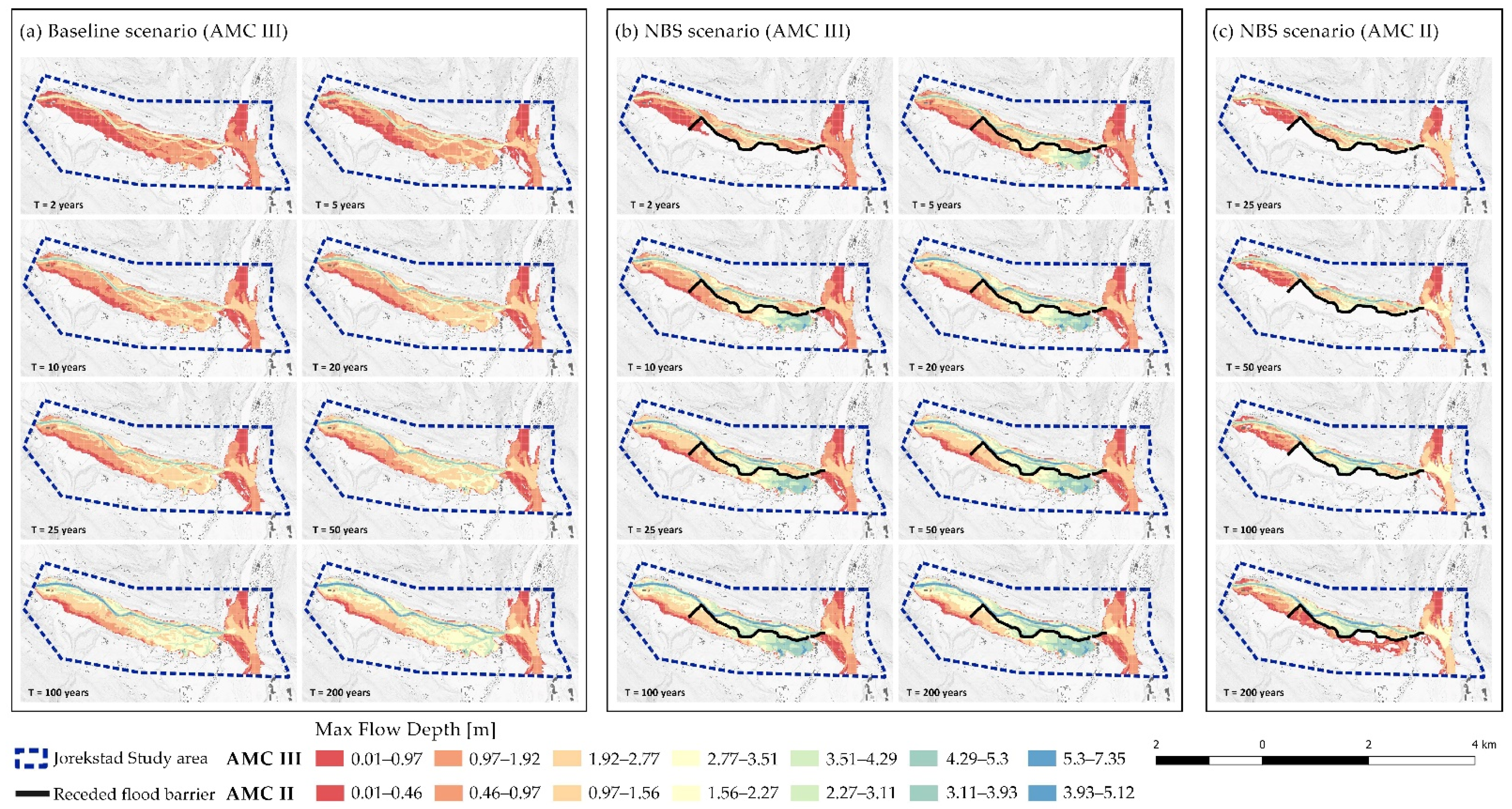
As the flood hazard simulation target was to forecast the maximum discharge at different return periods, a first simulation run was carried out considering the most severe situation of 5-day antecedent rainfalls, namely, AMC III.

In the baseline scenario, the flood plain was inundated at each return period. Starting from the 10-year return period, the flooded area threatened the sports facilities at Jorekstad. The average maximum flow depth ranged from 1.28 m in the 2-year return period (with an absolute maximum of 3.37 m in the floodplain) to 2.60 m in the 200-year return period (with an absolute maximum of 5.2 m in the floodplain). Concerning the average maximum flow velocity, it ranged from 0.40 m/s in the 2-year return period (with an absolute maximum of 0.50 m/s in the floodplain) to 0.57 m/s in the 200-year return period (with an absolute maximum of 0.84 m/s in the floodplain (Figure 3a)).

The NBS scenario simulation revealed how the receded flood barrier is able to prevent the floodplain inundation only when a 2-year return-period rainfall event occurs. In the other cases, the portion of the barrier perpendicular to the river was bypassed to the south by the flood, and the levee was almost totally overstepped. Therefore, the flood plain was always fully inundated, and the Jorekstad sport center was threatened by the flood. Moreover, it did not contribute to limit flow depth and velocity. Actually, the average maximum flow depth ranged from 1.52 m in the 2-year return period (with an absolute maximum of 0.17 m in the small portion of the floodplain that was inundated) to 2.90 m in the 200-year return period (with an absolute maximum of 6.2 m in the floodplain). Similarly, the maximum flow velocity ranged from 0.51 m/s in the 2-year return period (with an absolute maximum of 0.40 m/s in the floodplain) to 0.60 m/s in the 200-year return period (with an absolute maximum of 1.6 m/s in the floodplain) (Figure 3b).

By comparing the total numbers of flooded areas in the baseline scenario and in the NBS one, it was observed that the flood barrier might actually increase the flooded area just after it is overstepped, i.e., starting from a 5-year return period. Similar results were observed when the levee was slightly modified by both prolonging its initial portion to the south and raising the barrier crown by 1 or 2 m.

A second simulation run was carried out considering the average situation of 5-day antecedent rainfall, AMC II, to assess the effectiveness of the flood barrier in less severe soil moisture conditions. In this case, the levee avoided the plain flooding for each return period not longer than 100 years. Furthermore, even in the case of a 200-year rainfall event, the extension of the flooded area was efficiently limited, and the flood did not threaten the Jorekstad settlements (Figure 3c).

4. Conclusions

Flooding is the major natural hazard threatening the Jorekstad study area and the river Gausa watershed. The methodology applied for flood hazard assessment in the frame of PHUSICOS project allowed generating high-resolution hazard maps of several stream flow conditions, such as flow velocity, flow depth and the extension of the possible flooded areas, for both the baseline and the NBS scenario, at different soil moisture conditions. Through FLO-2D modelling, the flooded areas were detected, and the maximum flow depth and the velocity were assessed for each analyzed 20 m of the study area at 2, 5, 10, 20, 25, 50, 100 and 200-year return periods.

In the most severe soil moisture conditions (AMC III), the flood barrier proved to be ineffective against rainfall events having return periods longer or equal to 5 years. Moreover, it showed the opposite effect of reducing stream flow conditions, since the flow overstepping the barrier was no longer spilled into the river. This provoked higher maximum flow depth and velocity and bigger flooded areas than in the baseline scenario.

Different physical features of the barrier (+140 m long, +2 m high) did not contribute to enhance its effectiveness. It is worth nothing that raising the earth barrier crown more than 2 m would not be technically and economically feasible, since its 2:1 sloped sides would entail a much greater footprint.

In average soil moisture conditions (AMC II), the simulations revealed how the planned NBS was fully effective against flooding caused by rainfall events having a return period longer than 100 years. Even when 200-year rainfall events occur, the flood barrier would limit the flooded areas and protect the exposed settlements.

Future applications of the methodology herein discussed should account for the hydraulic model having an even higher resolution, as long as glitches, due to data processing capacity, can be easily overcome.

References

- Jonkman, S.N. Global Perspectives on Loss of Human Life Caused by Foods. Nat. Hazards 2005, 34, 151–175. [Google Scholar] [CrossRef]
- CRED. Natural Disasters 2018; Centre for Research on the Epidemiology: Brussels, Belgium, 2018. [Google Scholar]
- Groisman, P.Y.; Knight, R.W.; Easterling, D.R.; Karl, T.R.; Hegerl, G.C.; Razuvaev, V.N. Trends in Intense Precipitation in the Climate Record. J. Clim. 2005, 18, 1326–1350. [Google Scholar] [CrossRef]
- Eccles, R.; Zhang, H.; Hamilton, D. A Review of the Effects of Climate Change on Riverine Flooding in Subtropical and Tropical Regions. J. Water Clim. Chang. 2019, 10, 687–707. [Google Scholar] [CrossRef]
- Talbot, C.J.; Bennet, E.M.; Cassell, K.; Hanes, D.M.; Minor, E.C.; Paerl, H.; Raymond, P.A.; Vargas, R.; Vidon, P.; Wollheim, W.; et al. The Impact of Flooding on Aquatic Ecosystem Services. Biogeochemistry 2018, 141, 439–461. [Google Scholar] [CrossRef] [PubMed]
- Atta-ur-Rahman; Khan, A.N. Analysis of Flood Causes and Associated Socio-economic Damages in the Hindukush Region. Nat. Hazards 2011, 59, 1239–1260. [Google Scholar] [CrossRef]
- Akpoveta, V.O.; Osakwe, S.A.; Ize-Iyamu, O.K.; Medjor, W.O.; Egharevba, F. Post Flooding Effect on Soil Quality in Nigeria: The Asaba, Onitsha Experience. Open J. Soil Sci. 2014, 4, 72–80. [Google Scholar] [CrossRef][Green Version]
- Walls, R.L.; Heller Wardrop, D.; Brooks, R.P. The impact of experimental sedimentation and flooding on the growth and germination of floodplain trees. Plant Ecol. 2005, 176, 203–213. [Google Scholar] [CrossRef]
- Schneiderbauer, S.; Fontanella Pisa, P.; Delves, J.L.; Pedoth, L.; Rufat, S.; Erschbamer, M.; Thaler, T.; Carnelli, F.; Granados-Chahin, S. Risk perception of climate change and natural hazards in global mountain regions: A critical review. Sci. Total Environ. 2021, 784, 146957. [Google Scholar] [CrossRef]
- Mountain Research Initiative EDW Working Group. Elevation-dependent warming in mountain regions of the world. Nat. Clim. Change 2015, 5, 424–430. [Google Scholar] [CrossRef]
- UNISDR. Sendai framework for disaster risk reduction 2015–2030. In Proceedings of the Third United Nations World Conference on DRR, Sendai, Japan, 14–18 March 2015. [Google Scholar]
- EC Directorate-General for R&I. Evaluating the Impact of Nature-Based Solutions: A Handbook for Practitioners; Publications Office of the European Union: Luxembourg, 2021. [Google Scholar]
- Huang, Y.; Tian, Z.; Ke, Q.; Liu, J.; Irannezhad, M.; Fan, D.; Hou, M.; Sun, L. Nature-based Solutions for Urban Pluvial Flood Risk Management. WIREs Water 2020, 7, e1421. [Google Scholar] [CrossRef]
- Cohen-Shacham, E.; Walters, G.; Janzen, C.; Maginnis, S. Nature-Based Solutions to Address Global Societal Challenges; IUCN: Gland, Switzerland, 2016. [Google Scholar]
- Zölch, T.; Henze, L.; Keilholz, P.; Pauleit, S. Regulating urban surface runoff through nature-based solutions—An assessment at the micro-scale. Environ. Res. 2017, 157, 135–144. [Google Scholar] [CrossRef] [PubMed]
- PHUSICOS R&D Project—Horizon 2020. Available online: https://phusicos.eu/ (accessed on 10 September 2021).
- Oppland County Administration Regional Plans. Available online: https://innlandetfylke.no/_f/p1/i34056176-b265-41c3-a53b-e63f4b9ab5cb/lagen-plan_english_main-document.pdf (accessed on 7 October 2021).
- Solheim, A.; Capobianco, V.; Oen, A.; Kalsnes, B.; Wullf-Knutsen, T.; Olsen, M.; Del Seppia, N.; Arauzo, I.; Garcia Balaguer, E.; Strout, J.M. Implementing Nature-Based Solutions in Rural Landscapes: Barriers Experienced in the PHUSICOS Project. Sustainability 2021, 13, 1461. [Google Scholar] [CrossRef]
- De Paola, F.; Giugni, M.; Topa, M.E.; Bucchignani, E. Intensity-Duration-Frequency (IDF) Rainfall Curves, for Data Series and Climate Projection in African Cities. Springerplus 2014, 3, 133. [Google Scholar] [CrossRef] [PubMed]
- Erena, S.H.; Worku, H.; De Paola, F. Flood Hazard Mapping Using FLO-2D and Local Management Strategies of Dire Dawa city, Ethiopia. J. Hydrol. Reg. Stud. 2018, 19, 224–239. [Google Scholar] [CrossRef]
- Norwegian Mapping Authority. National Website for Map Data and Other Location Information in Norway. Kartverket. Available online: http:///www.geonorge.no (accessed on 1 October 2021).
- Natural Resources Conservation Service. National Engineering Handbook Part 630 Hydrology; United States Department of Agriculture: Washington, DC, USA, 2021. [Google Scholar]
- Ponce, V.M.; Hawkins, R.H. Runoff Curve Number: Has It Reached Maturity? J. Hydrol. Eng. 1996, 1, 11–19. [Google Scholar] [CrossRef]
- Soulis, K.X. Soil Conservation Service Curve Number (SCS-CN) Method: Current Applications, Remaining Challenges, and Future Perspectives. Water 2021, 13, 192. [Google Scholar] [CrossRef]
- Lal, M.; Mishra, S.K.; Pandey, A.; Pandey, R.P.; Meena, P.K.; Chaudhary, A.; Jha, R.K.; Shreevastava, A.K.; Kumar, Y. Evaluation of the Soil Conservation Service Curve Number Methodology Using Data from Agricultural Plots. Hydrogeol. J. 2017, 25, 151–167. [Google Scholar] [CrossRef]
- Simas, M. Lag Time Characteristics in Small Watersheds in the United States. A Dissertation Submitted to School of Renewable Natural Resources; University of Arizona: Tucson, AZ, USA, 1996. [Google Scholar]
- Mockus, V. Use of Storm and Watershed Characteristics in Synthetic Hydrograph Analysis and Application; American Geophysical Union: Sacramento, CA, USA, 1957. [Google Scholar]
- O’Brien, J.; Garcia, R. FLO-2D Reference Manual, Version 2009. Available online: https://docs.dicatechpoliba.it/filemanager/303/PROTEZIONE%20IDRAULICA%202016-2017/3.3_FLO-2D%20Reference%20Manual%202009.pdf (accessed on 7 October 2021).