Pressure-Driven Simulation of Water Distribution Networks: Searching for Numerical Stability ^†

Abstract

EPANET uses a demand-driven approach to compute pressures and flows in the water distribution system. The demand-driven approach (DDA) assumes that the required demand is always fully satisfied no matter the existing pressure. In scenarios of pressure-deficient conditions the DDA results are not accurate, and a pressure-driven approach (PDA) is needed. Frequently, the PDA is accomplished by using equations that compute the available demand/leakage as a function of the current pressure. However, embedding such equations into the solver introduces convergence problems. This paper details the actions taken in WaterNetGen—an EPANET extension—to bring numerical stability to the pressure-driven solver, namely, by smoothing the pressure–demand/leakage relationship and the pump curve.

1. Introduction

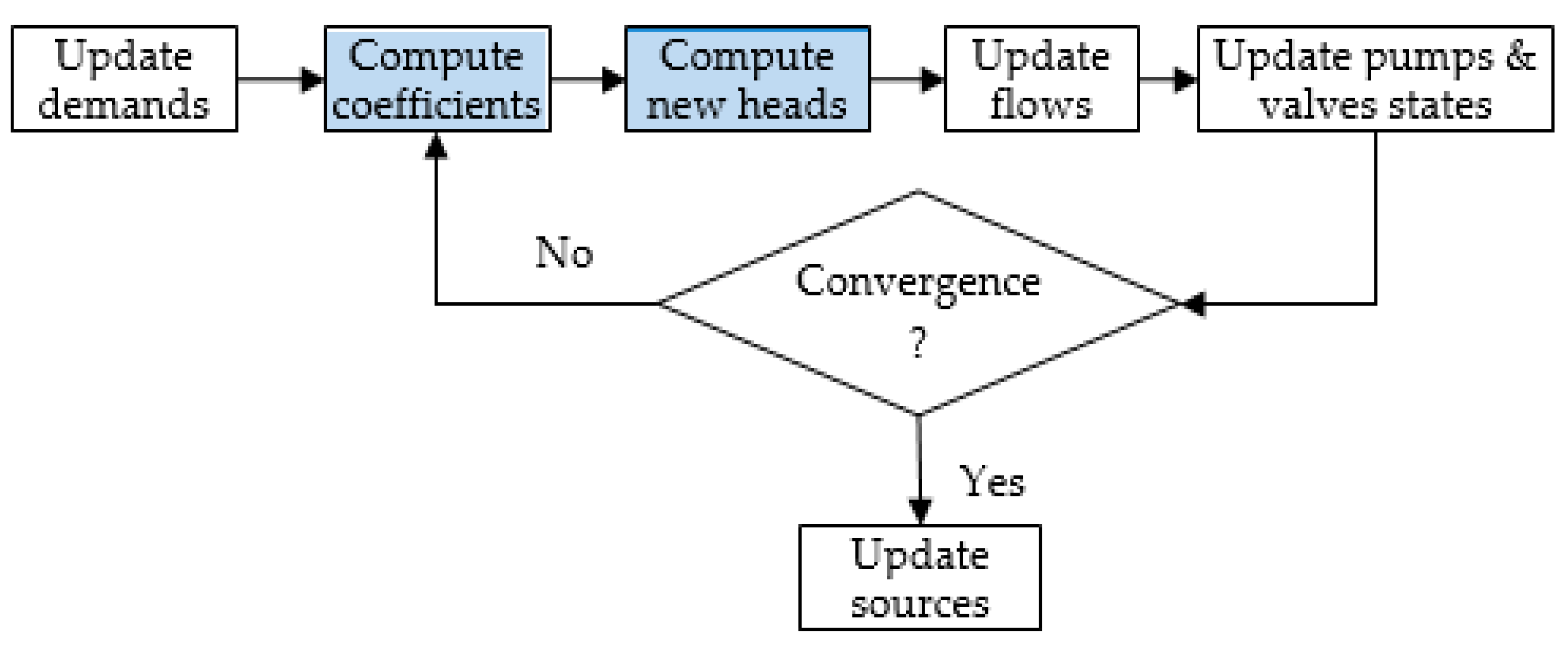
EPANET [1] is a public domain Windows software developed by the U.S. Environmental Protection Agency (USEPA). EPANET performs extended period simulations of the hydraulic and water quality behaviour of drinking water distribution systems. EPANET uses a link-node formulation, where consumption along the pipes is assigned to their end-nodes and defined as demand. 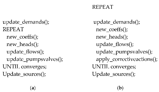To compute the nodal heads and the link flows, EPANET iteratively solves a linear system of equations until some convergence criterion is achieved—see Figure 1 and Listing 1a.

A linear system of equations results from the linearization of the mass conservation and energy equations by the Newton–Raphson method [2]. The iterative computation of Figure 1 stops when some level of accuracy is reached. Thus, the heads (and flows) are computed to satisfy the desired demand, which can lead to solutions with negative pressures. In other words, the demand is always satisfied independently of the available nodal pressure, even in the presence of negative pressures—a physical impossibility. Due to this behaviour, it is said that EPANET performs a Demand-Driven Analysis (DDA).

A better approach is to compute the demand as a function of the current pressure—Pressure-Driven Analysis (PDA). In this case, the iterative process must include the “Update demands” block from Figure 1—see Listing 1b.

Listing 1. Pseudocode for the iterative computation of heads and flows: (a) Demand-Driven; (b) Pressure-Driven.

The computation of the demand inside the loop frequently introduces numerical instability, which requires some corrective actions. In [3], the authors used a pressure–demand/leakage relationship to compute the available demand/leakage and employ relaxation coefficients to deal with these convergence difficulties. However, the authors concluded that in some cases the relaxation coefficients are not enough to guarantee convergence. This paper proposes a smoothing technique to build a differentiable pressure–demand/leakage relationship to improve the convergence of the iterative process.

The next section briefly introduces the Global Gradient Algorithm [2], its pressure-driven version [4] and the proposed smoothing technique to be applied to demands, leakages and pump curves computation. Section 3 includes some results. Section 4 concludes the paper and discusses some future developments.

2. Materials and Methods

At the core of the EPANET solver is the Global Gradient Algorithm (GGA). Section 2.1 introduces the EPANET solver, Section 2.2 describes the pressure-dependent changes to the GGA and Section 2.3 describes the smoothing technique proposed.

2.1. EPANET Solver

Considering a hydraulic network composed of np pipes with unknown flow rates, nn nodes with unknown heads and n0 nodes with known heads, the GGA states:

$$\left[\begin{array}{cc}{{\displaystyle A}}_{11}& {{\displaystyle A}}_{12}\\ {{\displaystyle A}}_{21}& 0\end{array}\right]\left[\begin{array}{c}Q\\ H\end{array}\right]=\left[\begin{array}{c}-{{\displaystyle A}}_{10}{{\displaystyle H}}_0\\ -q\end{array}\right],$$

(1)

where Q = [Q₁, Q₂, ..., Q_np]^T is the column vector of unknown pipe flow rates; H = [H₁, H₂, ..., H_nn]^T is the column vector of unknown nodal heads; H₀ = [H₀₁, H₀₂, ..., H_0n0]^T is the column vector of known nodal heads; and q = [q₁, q₂, ..., q_nn]^T is the column vector of known demands.

In Equation (1), A₁₁ is a np × np diagonal matrix whose elements correspond to the pipe head losses; A₁₂ = A₂₁^T and A₁₀ = A₀₁^T are the topological incidence matrices of size np × nn and np × n0, respectively.

Assuming a head loss formula as follows:

$${{\displaystyle h}}_i={{\displaystyle R}}_i\cdot {{\displaystyle Q}}_i{{\displaystyle \left|{{\displaystyle Q}}_i\right|}}^{{{\displaystyle n}}_i-1},$$

(2)

the A₁₁ matrix takes the form

$${{\displaystyle A}}_{11}=\left[\begin{array}{ccccc}{{\displaystyle R}}_1{{\displaystyle \left|{{\displaystyle Q}}_1\right|}}^{{{\displaystyle n}}_1-1}& & & & \\ & {{\displaystyle R}}_2{{\displaystyle \left|{{\displaystyle Q}}_2\right|}}^{{{\displaystyle n}}_2-1}& & & \\ & & \cdot & & \\ & & & \cdot & \\ & & & & {{\displaystyle R}}_{np}{{\displaystyle \left|{{\displaystyle Q}}_{np}\right|}}^{{{\displaystyle n}}_{np}-1}\end{array}\right],$$

(3)

Considering D₁₁ as the derivative of A₁₁ with respect to pipe flows, the iterative formulation to find a solution of (1) can be stated as follows:

$$\begin{array}{l}{{\displaystyle A}}^k={{\displaystyle A}}_{21}{{\displaystyle ({{\displaystyle D}}_{11}^k)}}^{-1}{{\displaystyle A}}_{12}\\ {{\displaystyle {{\displaystyle F}}^k={{\displaystyle (A}}_{21}Q}}^k-q)-{{\displaystyle A}}_{21}{{\displaystyle ({{\displaystyle D}}_{11}^k)}}^{-1}{{\displaystyle (A}}_{10}{{\displaystyle H}}_0+{{\displaystyle A}}_{11}^k{{\displaystyle Q}}^k)\\ {{\displaystyle H}}^{k+1}={{\displaystyle ({{\displaystyle A}}^k)}}^{-1}{{\displaystyle F}}^k\\ {{\displaystyle Q}}^{k+1}={{\displaystyle Q}}^k-{{\displaystyle ({{\displaystyle D}}_{11}^k)}}^{-1}{{\displaystyle ({{\displaystyle A}}_{11}^k{{\displaystyle Q}}^k+{{\displaystyle A}}_{12}{{\displaystyle H}}^{k+1}+A}}_{10}{{\displaystyle H}}_0)\end{array}$$

(4)

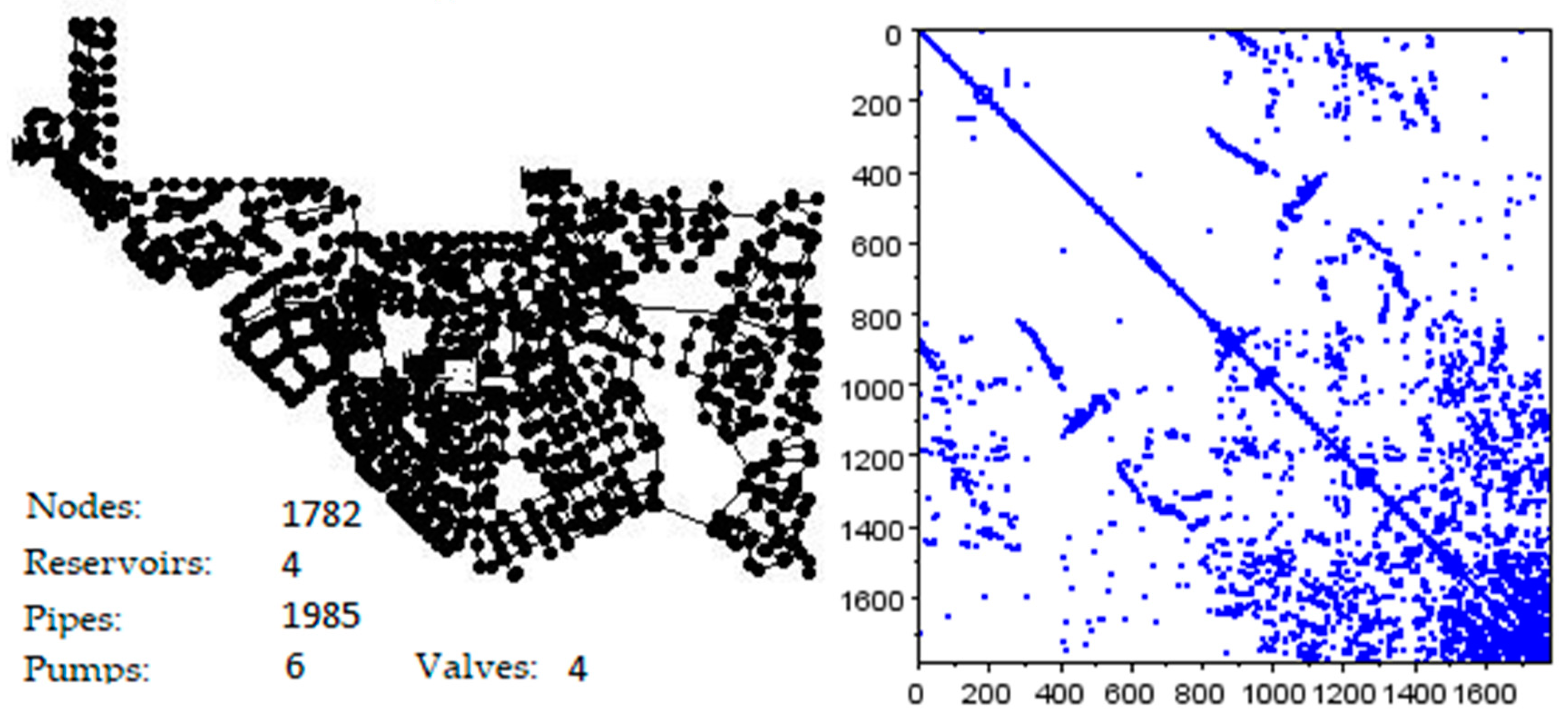
The computation of the new head, H^k+1, corresponds to solving a system of linear equations Ax = b, with A = A^k, x = H^k+1 and b = F^k, where the coefficients matrix A is sparse, symmetric and positive definite—see Figure 2. EPANET solves this linear system through a direct method (LL^T—Cholesky factorization) customised to sparse matrices.

The EPANET implementation of the linear system solver first applies an ordering (Minimum Degree) algorithm to reduce the fill-in problem linked to the factorization of sparse matrices [6]. Figure 2 shows the matrix sparsity pattern that results from the ordering phase (and before numerical factorization) of the benchmark network Wolf–Cordera Ranch.

2.2. Pressure-Dependent Demand

There are two types of pressure dependent demands to be considered: the demand itself and pipe leakage. The pressure-dependent demand for a node i can be computed by the following relationship [7]:

$$q_i^{avl}\left(P_i\right)=q_i^{req}\times DSR(P_i,P_i^{min},P_i^{ref},\alpha ),$$

(5)

where P_i^ref is the reference (or service) pressure necessary to fully satisfy the required demand q_i^req, P_i^min is the pressure below which no water can be supplied, P_i is the current pressure at node i and DSR (Demand Satisfaction Ratio) is the ratio between the available and the required demands defined by

$$DSR(P_i,P_i^{min},P_i^{ref},\alpha )=\{\begin{array}{cc}1& P_i\ge P_i^{ref}\\ {\left(\frac{P_i-P_i^{min}}{P_i^{ref}-P_i^{min}}\right)}^{\alpha }& P_i^{min}<P_i<P_i^{ref}\\ 0& P_i\le P_i^{min}\end{array},$$

(6)

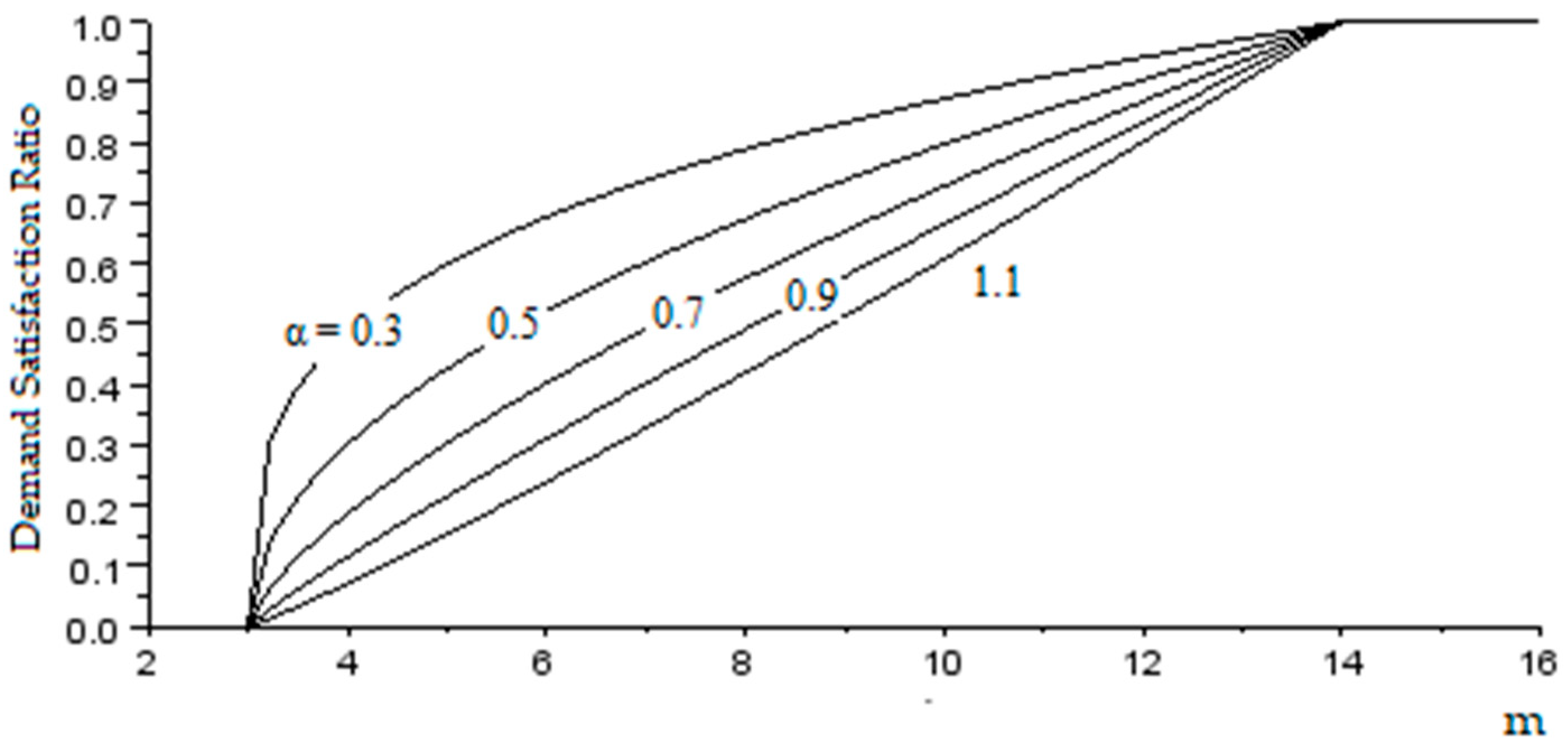
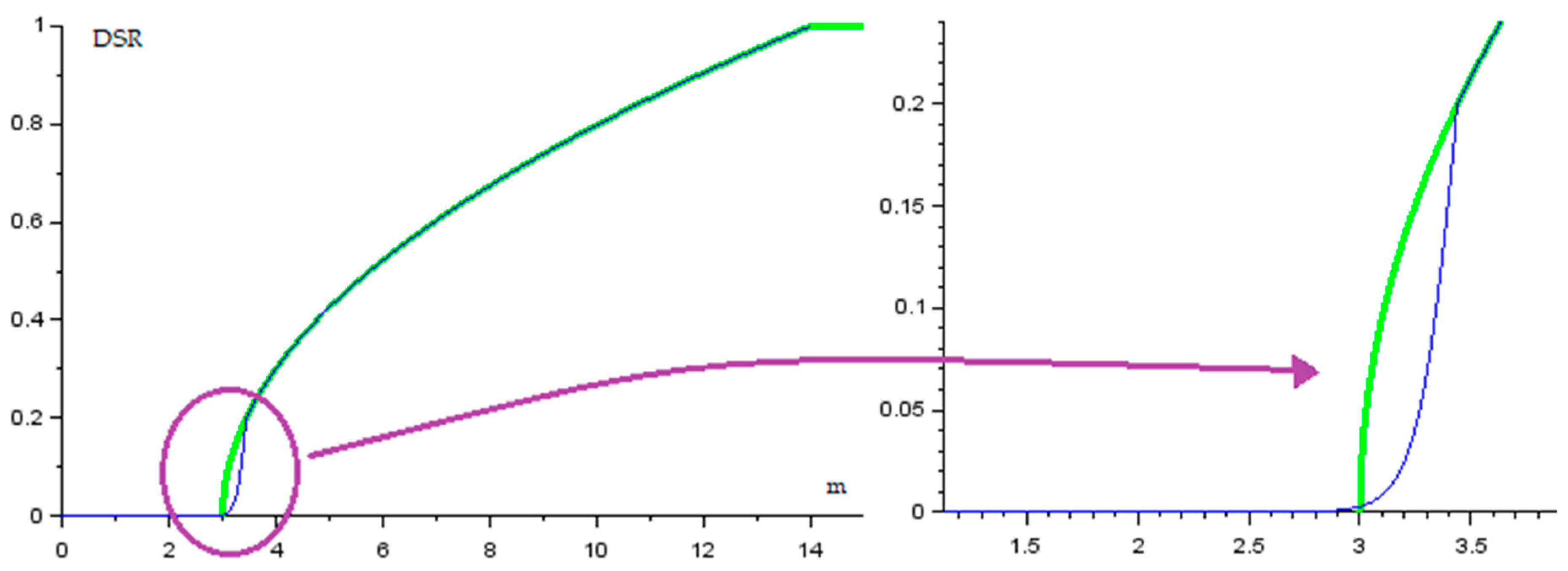
The exponent of the pressure–demand relationship, α, typically assumes the value 0.5, but should be set by calibration. Figure 3 illustrates the DSR for different values of the exponent and considering P^min = 3 m and P^ref = 14 m.

Leakage also depends on the pressure. In fact, leakage increases when pressure rises and decreases when pressure falls. The pipe leakage can be expressed by the sum of two components: background leakage and bursts leakage. The pressure–leakage relationship can be set as follows [8]:

$$q_k^{leak}\left(P_k\right)=\{\begin{array}{cc}{{\displaystyle \beta }}_k{{\displaystyle l}}_k{{\displaystyle (P_k)}}^{{{\displaystyle \alpha }}_k}+{{\displaystyle C}}_k{{\displaystyle (P_k)}}^{{{\displaystyle \delta }}_k}& P_k>0\\ 0& P_k\le 0\end{array},$$

(7)

where q_k^leak is the total leakage flow along pipe k; l_k is the length of pipe k; α_k and β_k are parameters of the background leakage model; C_k and δ_k are parameters of the bursts leakage model (classical orifice flow formulas); and P_k is the average pressure in pipe k computed as the arithmetic mean of the pressure values of its end nodes. According to Lambert [9], the α_k parameter can take values between 0.5 and 2.5, depending on the leak type. The β_k parameter is related to the pipe material deterioration, and its value must be set by calibration (initial values can be set around 10⁻⁷).

The iterative formulation for the PDA is as follows:

$$\begin{array}{l}{{\displaystyle DDL}}_{22}^k={{\displaystyle D}}_{22}^k+{{\displaystyle DL}}_{22}^k\\ {{\displaystyle A}}^k={{\displaystyle A}}_{21}{{\displaystyle ({{\displaystyle D}}_{11}^k)}}^{-1}{{\displaystyle A}}_{12}-{{\displaystyle DDL}}_{22}^k\\ {{\displaystyle {{\displaystyle F}}^k={{\displaystyle [A}}_{21}Q}}^k-({{\displaystyle q}}_{avl}^k-{{\displaystyle q}}_{leak}^k)]-{{\displaystyle A}}_{21}{{\displaystyle ({{\displaystyle D}}_{11}^k)}}^{-1}{{\displaystyle (A}}_{10}{{\displaystyle H}}_0+{{\displaystyle A}}_{11}^k{{\displaystyle Q}}^k)-{{\displaystyle DDL}}_{22}^k{{\displaystyle H}}^k\\ {{\displaystyle H}}^{k+1}={{\displaystyle ({{\displaystyle A}}^k)}}^{-1}{{\displaystyle F}}^k\\ {{\displaystyle Q}}^{k+1}={{\displaystyle Q}}^k-{{\displaystyle ({{\displaystyle D}}_{11}^k)}}^{-1}{{\displaystyle ({{\displaystyle A}}_{11}^k{{\displaystyle Q}}^k+{{\displaystyle A}}_{12}{{\displaystyle H}}^{k+1}+A}}_{10}{{\displaystyle H}}_0)\end{array}$$

(8)

where DL₂₂ and D₂₂ are the derivatives of q_leak and q_avl functions, Equations (5)–(7), with respect to pipe pressures and nodal pressures, respectively, and k is the current step.

WaterNetGen [4,10] uses relaxation coefficients to improve PDA convergence.

2.3. Function Smoothing

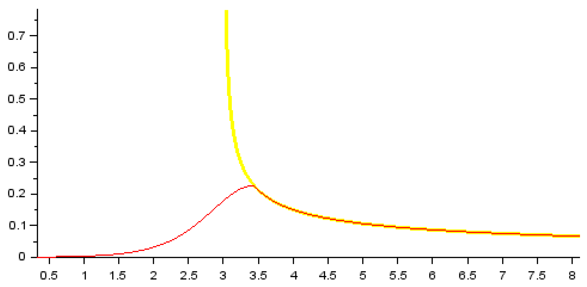
Despite the incorporation of relaxation coefficients in the pressure-dependent formulation, the PDA still evidences problems in some cases [3]. One source of such problems is the inclusion of the derivative terms of Equations (5)–(7) in the iterative process. For example, considering expression (6), when the current pressure approaches the minimum required pressure (P^min), the derivative tends to infinity. These derivative terms should be smoothed.

One way of dealing with ill-conditioned behaviour derivative terms is to cut part of the pressure–demand relationship extremity. Figure 4 illustrates the idea for the DSR (6): the extremity is replaced by another well-behaved curve, chosen to be differentiable.

The logistic sigmoid function (Equation (9)) is a good candidate to this operation, because it is differentiable and can be parametrised. Thus, the logistic function can be implanted at an appropriate location of the original function, for example, at a point X₀ corresponding to a DSR of 20%.

$$\begin{array}{l}f(x)=\frac{1}{1+{{\displaystyle e}}^{-\frac{{{\displaystyle x}}_{}-{{\displaystyle X}}_0}{K}}}\\ f’(x)=\frac{f(x)(1-f(x))}{K}\end{array}$$

(9)

The value of K can be computed to guarantee smooth derivatives too:

$$K=\frac{{{\displaystyle (P_i^{ref}-P_i^{min})}}^{\alpha }}{2\cdot \alpha {{\displaystyle (X_0-P_i^{min})}}^{\alpha -1}},$$

(10)

Figure 5 shows the graph of derivatives of the original and the smoothed functions and yellow and red lines, respectively.

The above function smoothing technique is a little elaborate to be applied to pressure–leakage functions. Thus, following the same idea of function smoothing, a pragmatic approach results: use the cubic Hermite interpolation [11]. Cubic Hermite curves provide continuity of first-order derivatives and match the set of (chosen) slopes. They are simple to calculate and only need two control points and two control tangents. Accordingly, two points can be considered x₁ = P^min and x₂ = x₁ + Δ, with function values f₁ = DSR(x₁, P^min, P^max, 0.5) = 0.0 and f₂ = DSR(x₂, P^min, P^max, 0.5). The Δ can be selected to produce a good smooth derivative curve (Figure 5). The corresponding tangent points, df₁ and df₂, can be set to a small value (for example, 1 × 10⁻¹⁰) and to the derivative of DSR on x₂, respectively. The curve coefficients (a, b, c, d) can be obtained by solving the following linear system:

$$\left[\begin{array}{cccc}{{\displaystyle x}}_1^3& {{\displaystyle x}}_1^2& {{\displaystyle x}}_1^{}& 1\\ {{\displaystyle x}}_2^3& {{\displaystyle x}}_2^2& {{\displaystyle x}}_2^{}& 1\\ {{\displaystyle 3x}}_1^2& {{\displaystyle 2x}}_1^{}& 1& 0\\ {{\displaystyle 3x}}_2^2& {{\displaystyle 2x}}_2^{}& 1& 0\end{array}\right]\left[\begin{array}{c}a\\ b\\ c\\ d\end{array}\right]=\left[\begin{array}{c}{{\displaystyle f}}_1\\ {{\displaystyle f}}_2\\ {{\displaystyle df}}_1\\ {{\displaystyle df}}_2\end{array}\right],$$

(11)

which is equivalent to computing

$$\begin{array}{l}a=\frac{2({{\displaystyle f}}_2-{{\displaystyle f}}_1)-({{\displaystyle x}}_2^{}-{{\displaystyle x}}_1^{})({{\displaystyle df}}_1+{{\displaystyle df}}_2)}{{{\displaystyle x}}_1^3-{{\displaystyle x}}_2^3+{{\displaystyle 3x}}_1^{}{{\displaystyle x}}_2^{}({{\displaystyle x}}_2^{}-{{\displaystyle x}}_1^{})}\\ b=\frac{({{\displaystyle df}}_2-{{\displaystyle df}}_1)-3({{\displaystyle x}}_2^2-{{\displaystyle x}}_1^2)\cdot a}{2({{\displaystyle x}}_2^{}-{{\displaystyle x}}_1^{})}\\ c={{\displaystyle df}}_1-{{\displaystyle 3x}}_1^2\cdot a-{{\displaystyle 2x}}_1^{}\cdot b\\ d={{\displaystyle f}}_1-{{\displaystyle x}}_1^3\cdot a-{{\displaystyle x}}_1^2\cdot b-{{\displaystyle x}}_1^{}\cdot c\end{array}$$

(12)

In WaterNetGen, the cubic Hermite curve, with the necessary adjustments, is applied to both extremities of the DSR function, to leakage (background and burst) components and to the pump curves.

3. Results

WaterNetGen is an EPANET extension that allows both demand-driven and pressure-driven simulations. The PDA is achieved with pressure–demand/leakage relationships (Equations (6)–(8)) and with relaxation coefficients. However, in a previous work [3] the authors found that in certain cases the process did not converge. These cases are related to valve interactions and to problems with the derivative terms.

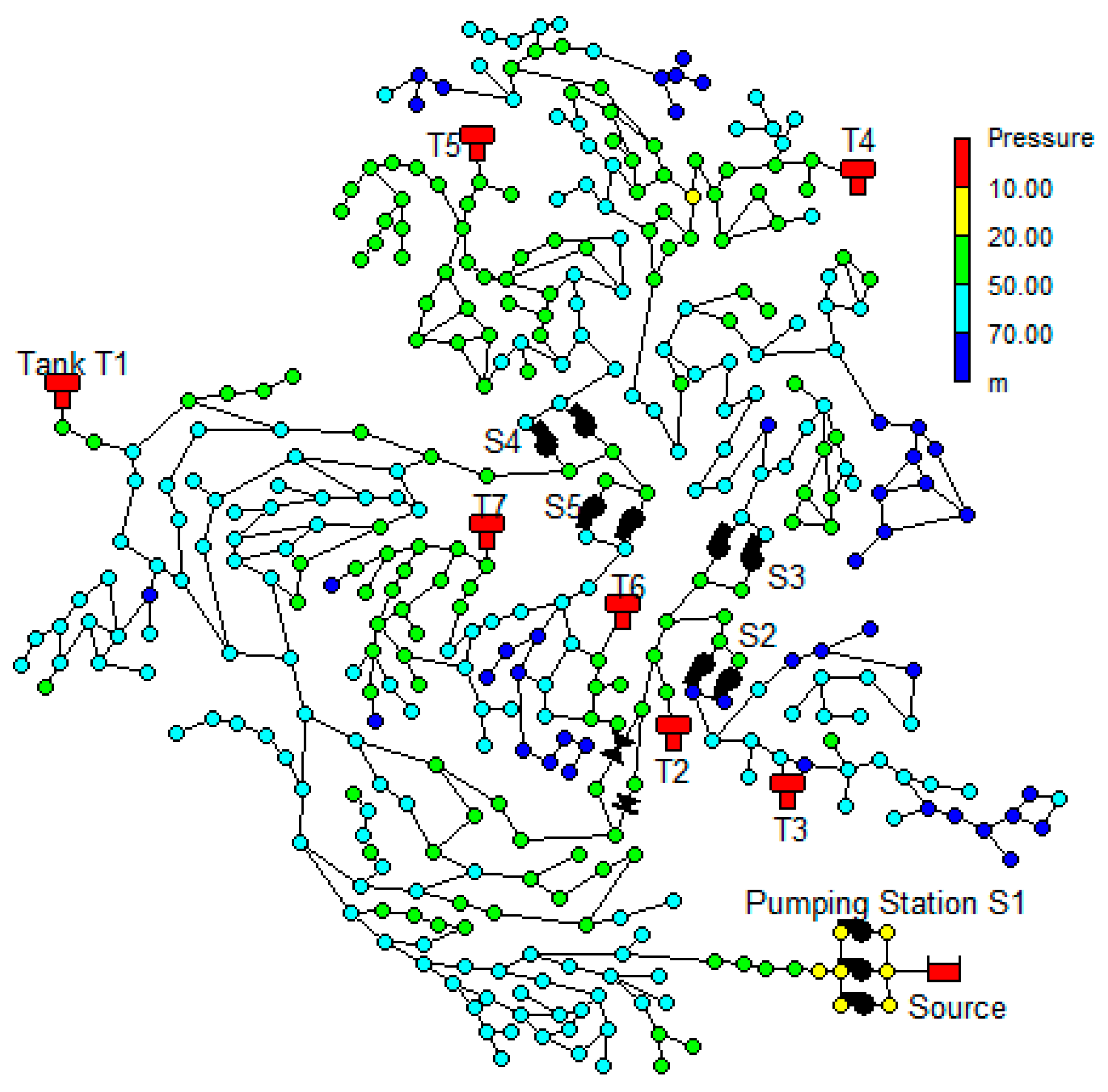
Figure 6 shows the C-Town network, used in the Battle of Background Leakage Assessment for Water Networks (BBLAWN) [12], where WaterNetGen was used to define a pump scheduling in order to minimise the operational costs (energy) and background leakage. In some runs WaterNetGen revealed some difficulties and did not converge.

The tool with the proposed smoothing technique is running again and almost does a decent job. However, there remain some cases where the process does not converge. That is, although there are improvements in the number of successful runs, there are still cases that deserve more research.

One final note about the research. The EPANET 2.2 [13], released on December 2019, comes with PDA capability based on Equations (5) and (6). This new version was used to simulate the behaviour of the BBLAWN network, but the result is always “WARNING: System unbalanced at…”. Therefore, this new version of EPANET still needs some reworking to deal with more complex networks.

4. Discussion and Conclusions

EPANET is the outstanding tool to study water distribution networks. However, EPANET is built around the demand-driven approach, which is not suitable to simulate pressure-deficient scenarios or pipe leakage. For these cases, the demand cannot be considered as constant known value, but instead must be considered as pressure dependent. A common way of specifying pressure-dependent demand is to consider a pressure–demand relationship and use it in the (iterative) simulation process.

The embedding of the pressure–demand relationship into the iterative process introduces instabilities in the solver. In the past, the authors tried to circumvent these instabilities with the inclusion of relaxation coefficients, which revealed to be essential to the convergence of the solver. Nevertheless, there persist some cases in which the solver does not converge.

The smoothing technique proposed in this work allowed one to overcome some more cases of lack of convergence. However, it is not a finished subject; there remain some cases not solved, so more research is needed.

In the future, the authors plan to add a backtracking algorithm, to assure global convergence for the Newton–Raphson method, and exploit it in combination with the techniques here introduced.