Article

Machine Learning Approaches for Soil Moisture Prediction Using Ground Penetrating Radar: A Comparative Study of Tree-Based Algorithms

by
Jantana Panyavaraporn
1,
Paramate Horkaew
2,
Rungroj Arjwech
3 and
Sitthiphat Eua-apiwatch
4,*
1
Department of Electrical Engineering, Faculty of Engineering, Burapha University, Chonburi 20131, Thailand
2
School of Computer Engineering, Suranaree University of Technology, Suranaree, Nakhon Ratchasima 30000, Thailand
3
Department of Geotechnology, Faculty of Technology, Khon Kaen University, Khon Kaen 40002, Thailand
4
Department of Civil Engineering, Faculty of Engineering, Burapha University, Chonburi 20131, Thailand
*
Author to whom correspondence should be addressed.
Earth 2025, 6(3), 98; https://doi.org/10.3390/earth6030098 (registering DOI)
Submission received: 28 June 2025 / Revised: 13 August 2025 / Accepted: 14 August 2025 / Published: 16 August 2025

Abstract

Accurate soil moisture estimation is critical for precision agriculture and water resource management, yet traditional sampling methods are time-consuming, destructive, and provide limited spatial coverage. Ground Penetrating Radar (GPR) offers a promising non-destructive alternative, but optimal machine learning approaches for GPR-based soil moisture prediction remain unclear. This study presents a comparative analysis of regression tree and boosted tree algorithms for predicting soil moisture content from Ground Penetrating Radar (GPR) histogram features across 21 sites in Eastern Thailand. Soil moisture content was measured at multiple depths (0.5, 1.0, 1.5, 2.0, 2.5, and 3.0 m) using samples collected during Standard Penetration Test procedures. Feature extraction was performed using 16-bin histograms from processed GPR radargrams. A single regression tree achieved a cross-validation RMSE of 5.082 and an R2 of 0.761, demonstrating superior training accuracy and interpretability. In contrast, the boosted tree ensemble achieved significantly better generalization performance, with a cross-validation RMSE of 4.7915 and an R2 of 0.708, representing a 5.7% improvement in predictive performance. Feature importance analysis revealed that specific histogram bins effectively captured moisture-related variations in GPR signal amplitude distributions. A comparative evaluation demonstrates that while single regression trees offer superior interpretability for research applications, boosted tree ensembles provide enhanced predictive performance that is essential for operational deployment in precision agriculture and hydrological monitoring systems.

1. Introduction

Precision agriculture and environmental monitoring require accurate estimation of soil moisture, but spatial coverage remains limited due to the time-consuming and destructive nature of traditional sampling. Non-destructive approaches offer promising alternatives for soil moisture estimation [1]. GPR technology enables high-resolution stratigraphy mapping and borehole data extension [2], supporting the transition toward non-invasive soil characterization methods. This limitation significantly impacts agricultural decision-making and water management efficiency. Non-destructive alternatives with a high resolution are offered by ground-penetrating radar (GPR) with accompanying machine-learning algorithms. Current methods predominantly rely on empirical relationships between dielectric permittivity and water content, which have received extensive experimental validation across diverse soil conditions [3,4,5,6,7]. However, systematic comparative evaluations of machine learning architectures for GPR-based soil moisture prediction remain limited in the literature [8,9,10,11,12,13]. This study compares single regression trees and boosted-tree ensemble regression to predict soil moisture using GPR data obtained through histogram features recorded at 21 different sites in Eastern Thailand. The main hypothesis of the current work is that compared to single regression trees, boosted-tree ensembles will perform better in terms of generalization. However, this comes at the expense of reduced interpretability.
This study addresses the research gap through the following specific objectives:
  • Systematically compare single regression trees versus boosted tree ensembles for soil moisture prediction using GPR histogram features from 21 Eastern Thailand sites;
  • Determine the performance trade-offs between model interpretability and predictive accuracy for operational deployment guidance;
  • Assess model reliability through uncertainty analysis and cross-validation across diverse soil categories (coastal sandy, transitional mixed, inland clayey).
To address these objectives, the study first establishes the theoretical foundation through a literature review, then develops a systematic methodology for comparative algorithm evaluation using field data from diverse geological conditions in Eastern Thailand. The analysis proceeds with comprehensive performance assessment and uncertainty quantification, followed by a discussion of the practical implications for precision agriculture and infrastructure monitoring applications.

2. Literature Review

2.1. Soil Moisture Estimation Using GPR

Ground-penetrating radar has played a crucial role in soil moisture characterization due to the strong reflection of dielectric properties of the subsurface through the propagation of electromagnetic waves. Empirical relationships between dielectric constants and volumetric water content have been established and continue to form the basis of current modeling approaches [3]. Comprehensive documentation exists on key subsurface factors, including soil texture and pore-water content, that influence GPR responses [4]. Calibration functions emphasizing frequency sensitivity and site-specific processes have been developed to improve measurement accuracy [5].
Recent advances in signal processing have shown the effectiveness of different feature extraction methods. Frequency-domain analysis has demonstrated significant relationships (R2 = 0.89–0.97) between peak frequency shifts and soil moisture across various soil types [6]. Experimental validation of the Average Envelope Amplitude (AEA) technique shows high correlation coefficients (R2 = 0.9869) between GPR parameters and dielectric permittivity [7]. Wave velocity approaches have achieved moderate accuracy (R2 = 0.514) for field-scale soil moisture estimation [8]. Furthermore, site-specific parameter calibration of mixed-media models, as demonstrated in desert steppe environments, has been shown to significantly enhance the accuracy of GPR-based soil moisture estimation [9]. Beyond moisture quantification, GPR has been applied to identify anthropogenic alterations in soil structure, where amplitude reductions indicate compaction and porosity changes, providing valuable insight for soil management [10].
GPR frequency selection significantly influences measurement depth and resolution capabilities. Higher frequencies (400–1000 MHz) provide enhanced near-surface resolution but limited penetration depth, while lower frequencies (100–400 MHz) enable deeper investigation at reduced spatial resolution. The choice of antenna configuration and survey parameters directly affects data quality and interpretation accuracy, requiring careful consideration of site-specific conditions and measurement objectives.

2.2. Geophysical Data Analysis Using Machine Learning

Building upon these GPR measurement principles, machine learning techniques have emerged as powerful tools for automated interpretation and prediction. The application of machine learning in geophysical interpretation has grown significantly in recent years. Ensemble architectures using polarimetric SAR data have demonstrated strong performance with R2 values of 0.94 for training and 0.79 for validation [11]. Compact polarimetric features combined with Gaussian Process Regression have achieved R2 = 0.73 [12]. Comparative assessments demonstrate Random Forest consistently outperforming Support Vector Regression and Gradient Boosting across evaluation metrics, highlighting ensemble advantages over traditional methods.
Specifically, for GPR-based applications, comprehensive evaluations demonstrate that neural networks achieve the highest accuracy for soil moisture prediction [13]. RBF neural networks show superior performance over multiple regression, reducing errors from 28.36% to 7.83% [14]. Fuzzy logic integration with machine learning classifiers achieves 90% classification accuracy for volumetric water content prediction [15]. Recent work integrating multiple GPR-derived signal features into backpropagation neural networks has outperformed single-feature approaches (e.g., AEA and frequency-shift), achieving high coefficients of determination [16].
Tree-based machine learning methods have proven particularly effective for environmental regression tasks, with Random Forest emerging as a widely adopted ensemble method [17]. Boosting algorithms have extensive regression applications [18], with gradient-boosting theory providing the foundation for modern ensemble approaches [19]. Combined GPR and electromagnetic-induction data achieve RMSE < 0.14 g/cm3 for soil bulk density prediction, demonstrating ensemble model viability for geophysical applications [20]. Integration of proximal sensing datasets, such as UAV-derived vegetation indices with soil properties, has also been used for accurate field-scale crop growth prediction, supporting the role of machine learning in precision agriculture [21]. Furthermore, combining GPR with Sentinel-1 SAR has been shown to capture both localized moisture variation and broader spatial trends [22], while laboratory experiments coupling time-domain reflectometry with GPR have demonstrated the potential of multi-method approaches for high-resolution spatiotemporal monitoring [23].

2.3. Advanced GPR Signal Processing and Feature Extraction

While algorithmic advances have improved prediction capabilities, signal processing refinements continue to enhance data quality and feature extraction. New signal-processing designs have been aimed at advanced feature extraction to achieve better subsurface characterization. Numerical modeling studies have demonstrated that surface moisture significantly affects electromagnetic wave propagation, emphasizing the necessity of comprehending electromagnetic interactions in wet surroundings for accurate soil characterization. Real-time GPR processing methods utilizing frequency domain filtering and nonlinear optimization have been developed to correct surface moisture measurements, resulting in significant data quality improvements [24]. Multi-modal sensor fusion approaches combining GPR with thermal imaging have demonstrated improved performance through deep-learning and ensemble methods, emphasizing the importance of histogram-based features [25]. Intelligent adaptive GPR systems utilizing power spectral feature extraction have enhanced near-surface moisture forecasting capabilities using Random Forest and XGBoost models [26].
Advanced envelope detection methods have achieved mean relative errors of moisture ranging between 2.81 and 7.41% to depths up to 3 m [27]. These results support the feasibility of envelope amplitude and early-time signals for depth characterization while providing strong evidence for histogram-oriented feature extraction approaches. GPR-derived image classification has achieved 98.2% accuracy using CNN-based feature extraction combined with ensemble classifiers [28].

2.4. Comparative Algorithm Studies and Research Gaps

Despite these technological advances, systematic comparative studies evaluating different approaches remain limited. The field of soil moisture prediction through machine learning has grown tremendously over recent years. However, comparative evaluation studies that systematically evaluate and critically assess methodological choices remain rather limited. Data-fusion methods combining hyperspectral and simulated GPR data have been investigated for soil moisture estimation, achieving R2 = 0.833 using linear regression with 94 datapoints from four measurement plots [29]. This work focused primarily on data fusion strategies using simulated data rather than conducting direct algorithmic comparisons between ensemble and regression-tree methods, highlighting the need for more comprehensive comparative studies using real-world data to systematically evaluate different machine learning approaches for soil moisture prediction.
Several studies have contributed to understanding how soil properties influence GPR signals, thereby enhancing the theoretical development of algorithm design. Research on soil compaction effects has revealed high correlation between bulk density and electromagnetic wave velocity (r = 0.882, p = 0.020) [30]. Controlled experiments have demonstrated GPR’s capability to identify compaction heterogeneity, although analysis has relied on visual rather than automated assessment methods [31].
Infrastructure applications have provided additional insights into algorithm performance. Theoretically grounded electromagnetic mixing density prediction models have been developed with recording errors of 2.2–2.8% in pavement applications [32]. Comparative evaluations of electromagnetic models for material property estimation have shown that ensemble methods, such as the Al-Qadi, Lahouar and Leng (ALL) model, outperform simpler approaches [33]. However, these studies focused on pavement materials rather than soil moisture applications.
Recent reviews highlight the potential and limitations of both single-tree and ensemble-tree algorithms in geophysical parameter estimation. However, comparisons are usually not controlled or performed as head-to-head analyses. Most explorations underscore the capabilities of individual algorithms instead of systematically evaluating trade-offs. This gap makes it difficult to guide practitioners on algorithm selection for site-specific requirements, especially in Southeast Asian contexts where limited comparative research exists.
The identified limitations in existing comparative studies highlight the need for systematic evaluation of machine learning approaches for GPR-based soil moisture prediction. This study addresses these gaps through controlled comparison of single regression trees versus boosted tree ensembles using real-world field data across diverse geological conditions.

3. Methodology

The current study develops a methodological framework to address this research gap by introducing a systematic process to test soil moisture prediction algorithms based on GPR data. The methodology is organized into two main domains. The problem domain encompasses fundamental data acquisition and processing components, including study area selection, GPR data acquisition, soil sampling procedures, and signal processing. The solution domain focuses on histogram-based feature extraction, algorithm implementation, and evaluation, including a single regression tree approach, boosted tree ensemble methodology, and a comprehensive performance evaluation framework. This dual-domain structure provides clear separation between data foundation and algorithmic solution development. The framework overview for soil moisture prediction using GPR is presented in Figure 1.

3.1. Study Area and Site Selection

A comparative study between the algorithms was conducted on 21 sites located on natural-gas-pipeline infrastructure in Rayong and Chonburi provinces of Eastern Thailand. This pipeline infrastructure provided accessible locations for systematic soil sampling and GPR data collection across diverse geological conditions. The pipeline corridor allowed us to obtain representative soil samples from coastal sands to inland clays, providing the geological diversity necessary for robust algorithm validation. The numbered highways (3, 36, 331, 344) shown on the map represent major transportation routes that provided access to the natural gas pipeline infrastructure and study sites during field data collection. The location of sites is illustrated in Figure 2.

3.2. Field Data Collection

3.2.1. GPR Data Acquisition

The fieldwork used the MALA Easy Locator GPR-system with a 500 MHz antenna. The trace intervals were 0.05 m, and the time windows were kept at 100 nanoseconds. This was performed to improve reliability by using three measurements at each location. Figure 3a demonstrates the standard protocol of the survey used at all locations.

3.2.2. Soil Sampling and Laboratory Analysis

Simultaneously with GPR acquisition, Standard Penetration Test depth samples at 0–0.5, 0.5–1.0, 1.0–1.5, 1.5–2.0, 2.0–2.5, and 2.5–3.0 m were taken using split-spoon samplers. Gravimetric moisture content was determined using analytical methods where samples were oven-dried at 105 °C to a constant mass. The actual sample size achieved was 123, rather than the planned 126 samples. Three samples could not be recovered by split-spoon samplers due to encountering coarse-grained materials with high moisture contents. This is a common occurrence in field soil sampling that prevents effective sample recovery. Other samples were successfully collected and submitted for laboratory analysis. The Standard Penetration Test (SPT) sampling procedure at the test sites is presented in Figure 3b.

3.3. Data Preprocessing

3.3.1. GPR Radargram Processing

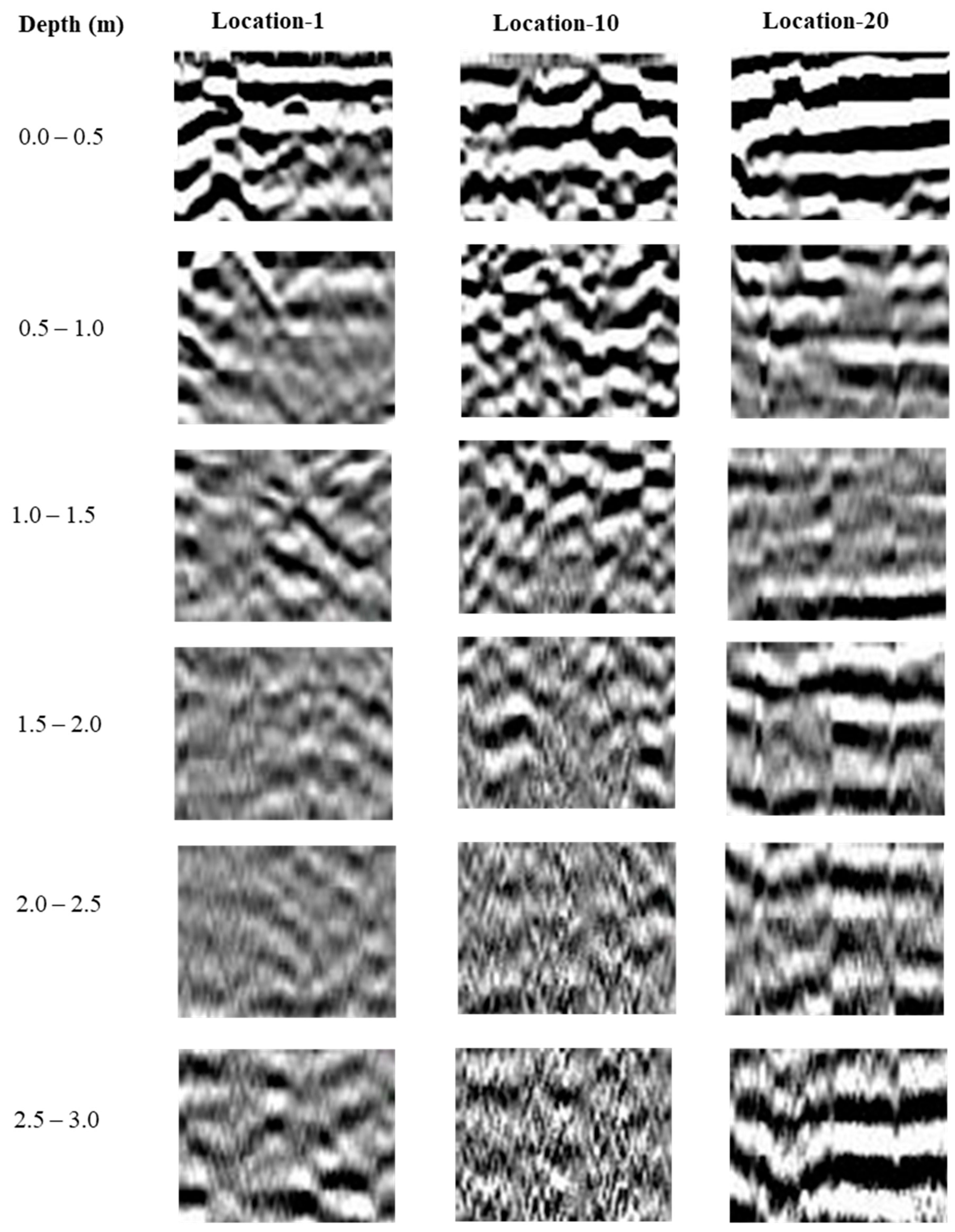
Radargrams were converted to 8-bit grayscale images. Figure 4 shows examples of GPR images at depths of 0.5, 1.0, 1.5, 2.0, 2.5, and 3.0 m, demonstrating the varying signal characteristics across different depths and geological conditions.

3.3.2. Histogram-Based Feature Extraction

A systematic evaluation was conducted using 4 to 24 bins to determine the optimal histogram configuration for feature extraction. The evaluation employed both a Single Regression Tree (with Pruning Level 10) and a Boosted Tree Ensemble (a maximum of 3 splits, 5 trees) to ensure robust parameter selection across both algorithmic approaches. A performance comparison across different histogram bin sizes is presented in Table 1.
A 16-bin configuration was selected based on its optimal balance between training accuracy and generalization capability across both algorithms. While a 24-bin configuration achieved higher training R2 values (0.778 and 0.734), the cross-validation RMSE results revealed signs of overfitting with deteriorating generalization performance (5.704 and 5.224). In contrast, the 16-bin configuration demonstrated stable cross-validation RMSE (5.082 and 4.792) while maintaining good training accuracy, indicating an optimal trade-off between model complexity and robustness. The 16-bin approach also provided sufficient granularity to capture moisture-related variations in GPR signal amplitude distributions without introducing excessive noise. Both algorithmic approaches showed consistent optimal performance in this configuration, confirming the robustness of this selection.
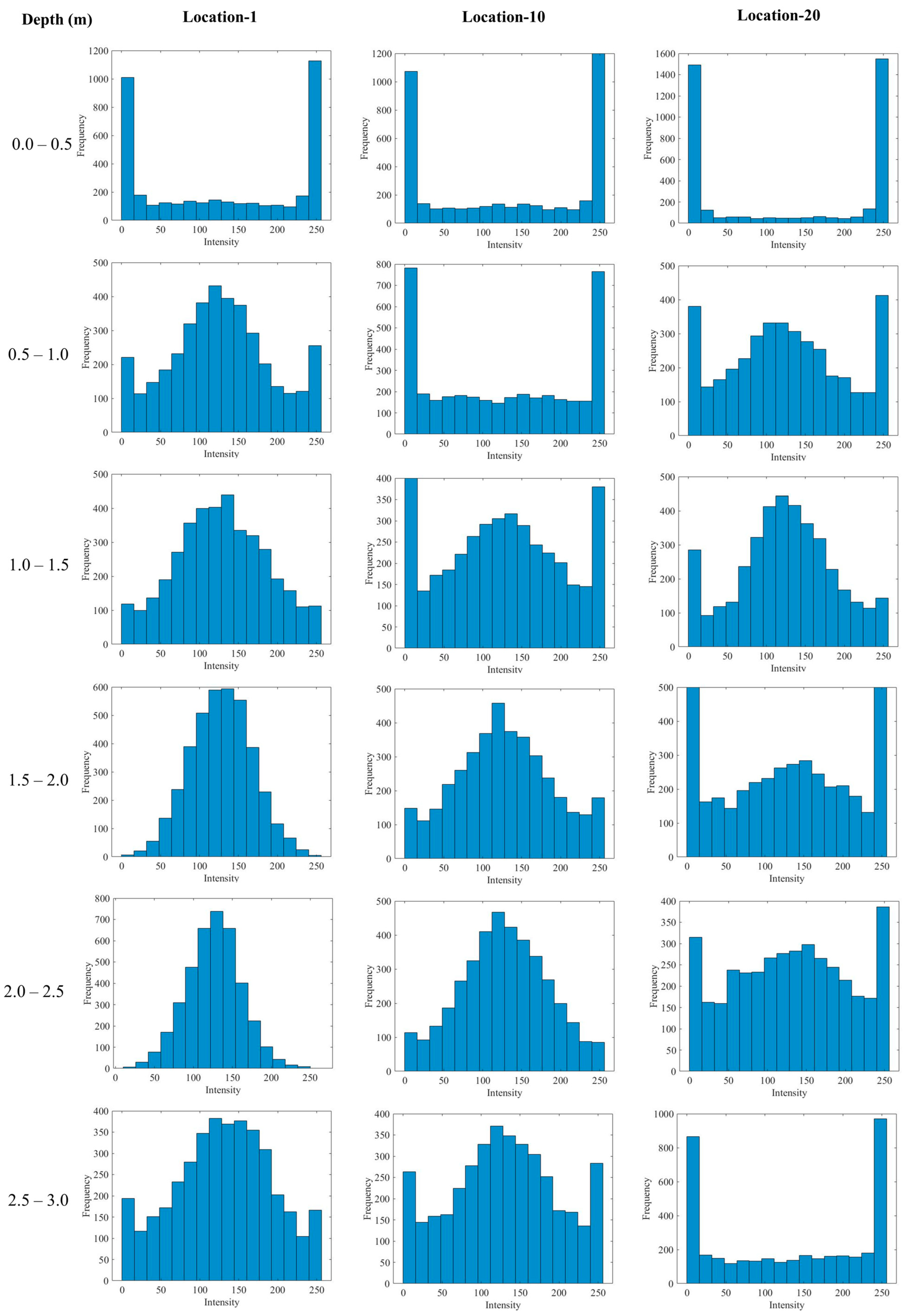
Feature extraction was based on 16-bin histogram analysis to capture the amplitude distribution of GPR images. Each radargram was divided into analysis windows corresponding to six specific depth intervals. For each window, a 16-bin histogram was computed to quantify the distribution of intensity values, which represent signal amplitudes designed to reflect variations in subsurface moisture content. Figure 5 presents examples of the resulting histograms corresponding to the GPR images at multiple depth intervals.

3.4. Machine Learning Implementation

3.4.1. Single Regression Tree Approach

The regression tree implementation used recursive data partitioning based on feature values, with the Mean Squared Error (MSE) as the splitting criterion, calculated as Equation (1)
M S E = 1 n i = 1 n y i y ¯ 2
where
n is the total number of samples in the node.
y i   is the actual target.
y ¯ is the mean of the target values in the node.
The optimal split is determined by minimizing the total weighted MSE after the split, given by Equation (2)
T o t a l M S E = n L n M S E L + n R n M S E R
Here, n L and n R refer to the number of samples in the left and right child nodes, respectively. M S E L and M S E R are the respective mean squared errors, and n is the total number of samples in the parent node. The systematic optimization approach involved data preparation, defining pruning levels from 4 to 14, cross-validation with pruning level tuning using 5-fold cross-validation, and final model training to identify optimal model complexity.

3.4.2. Boosted Tree Ensemble Approach

Boosted regression trees were implemented using the least squares boosting algorithm with sequential addition of weak learners. For regression tasks, the least squares error (L) is defined as Equation (3).
L y , y ^ = 1 2 y y ^ 2
where y is the true value of the target variable. y ^ is the predicted value from the model. Given a dataset with input (x) and a continuous target (y), the goal is to build an additive model using Equation (4).
F M x = m = 1 M λ m h m x
where F M x   is the final prediction after M boosting iterations, h m x   is the decision tree trained at iteration m, and λ m   is the step size or learning rate. At each iteration (m), the algorithm computes the residuals using Equation (5).
r i m = L y i , F x i F x i F x = F m 1 x
For least squares regression, Equation (5) was simplified to Equation (6).
r i m = y i F m 1 x i
A new tree h m x   is trained to predict the residuals. The model is updated by adding the new tree’s output, scaled by a learning rate λ 0,1 .
F M x = F m 1 x + λ h m x
The learning rate controls how much influence each tree has on the final model. A smaller learning rate leads to slower learning but often results in better generalization. The final output of the boosted model is a weighted sum of all the trees. The method allows the capture of complex, nonlinear relationships and is particularly effective for structured data. Boosted regression trees achieve high prediction accuracy by iteratively refining the model through gradient descent on the loss function. Each tree incrementally corrects the errors of its predecessors, resulting in a model capable of handling a wide range of regression tasks while reducing the risk of overfitting through various regularization mechanisms.
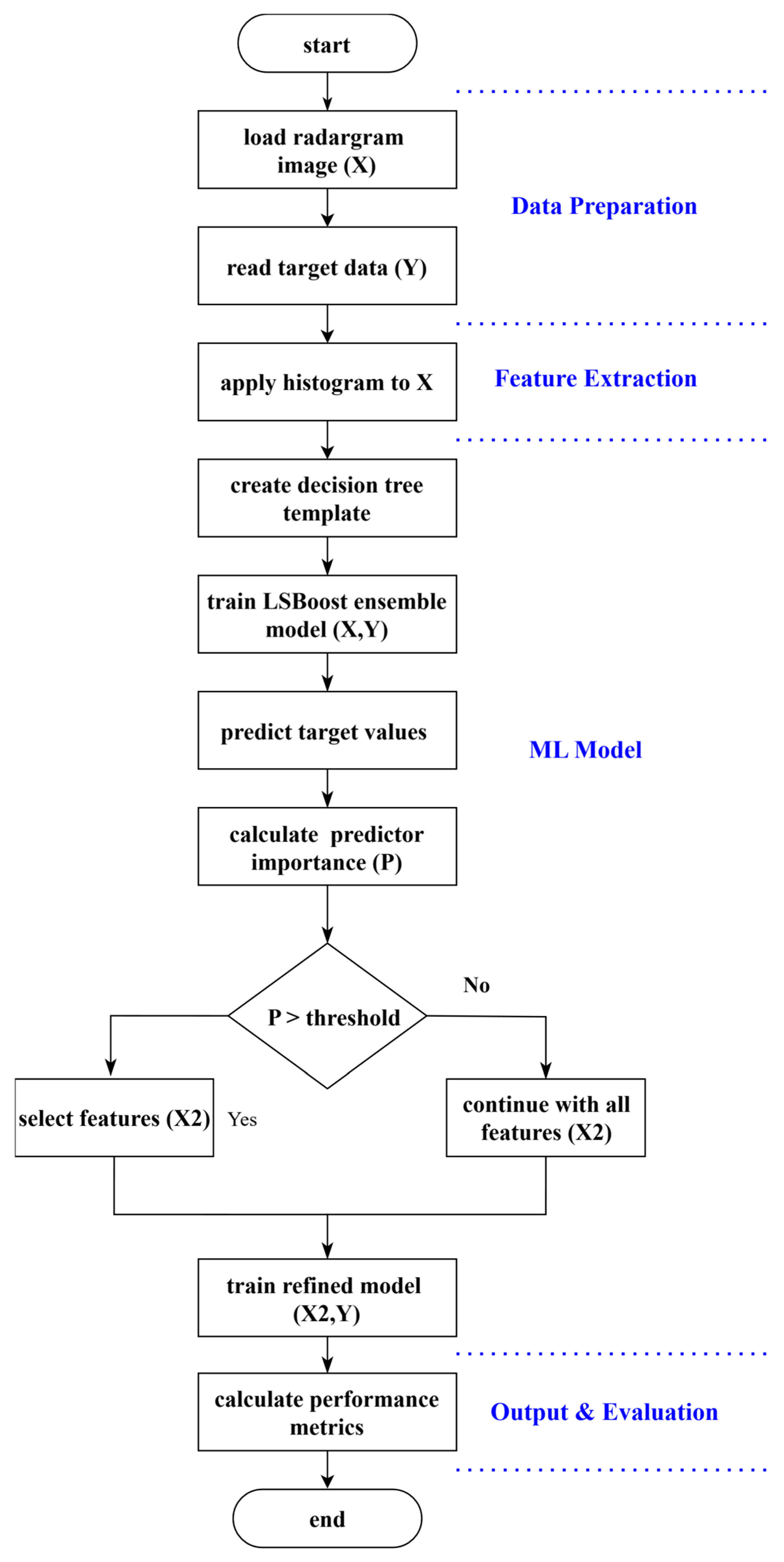
Figure 6 illustrates the complete boosted tree ensemble implementation process, including data preparation, histogram processing, model training, feature selection based on predictor importance thresholds, and performance evaluation. Hyperparameters, including maximum number of splits (1–15) and learning cycles (1–15), were optimized through a systematic grid search with 5-fold cross-validation.

3.5. Performance Evaluation

Algorithm comparison was performed using three key performance metrics, Root Mean Square Error (RMSE) assessed overall prediction accuracy; R-squared (R2) measured the proportion of variance explained by each model; and Mean Absolute Error (MAE) quantified average prediction deviations. These metrics provide complementary perspectives on algorithmic performance for soil moisture prediction applications.
  • Root Mean Square Error (RMSE) is used to evaluate the overall prediction accuracy by measuring the square root of the difference between the predicted and true values, as shown in Equation (8).
R M S E = 1 n i = 1 n y i y ^ i 2
  • R-squared (R2) represents the proportion of the variance in the observed data that is explained by the model, reflecting the explanatory power of the model, as shown in Equation (9).
R 2 = 1 i = 1 n y i y ^ i 2 i = 1 n y i y ¯ 2
  • Mean Absolute Error (MAE) represents the average of the predicted errors, providing a measure of model accuracy that can be interpreted in terms of absolute deviation, as shown in Equation (10).
M A E = 1 n i = 1 n y i y ^ i
where
n is the total number of samples;
y i is the true value of the ith sample;
y ^ i is the predicted value of the ith sample;
y ¯   is the mean of the true values.
K-fold cross-validation involves dividing the dataset into k subsets and systematically rotating the roles of the training and validation sets in each iteration. This approach reduces overfitting and ensures that the resulting performance metrics accurately reflect the generalizability of the model. It also provides a consistent and fair basis for comparing different algorithms using the same dataset.
The evaluation framework assessed training performance versus generalization capability, model interpretability, and computational efficiency. Cross-validation was implemented to ensure robust performance assessment and avoid overfitting, with the primary outcome variable being cross-validation RMSE for algorithm comparison.

4. Results

4.1. Site Characteristics and Data Collection

This study collected data from 21 sites across three geological soil types, coastal sandy (8 sites), transitional mixed (8 sites), and inland clayey (5 sites). Table 2 summarizes the diverse geological conditions encountered, ensuring comprehensive dataset variability for robust algorithm evaluation.

4.2. Algorithm Optimization Results

4.2.1. Single Regression Tree Optimization

Table 3 shows model performance across various pruning levels for single regression trees, identifying Level 10 pruning as optimal with cross-validation RMSE = 5.082 and R2 = 0.761.
Level 10 pruning was selected as optimal due to superior cross-validation performance while maintaining strong training accuracy (Table 3). This indicated the best balance between model complexity and generalization capability.
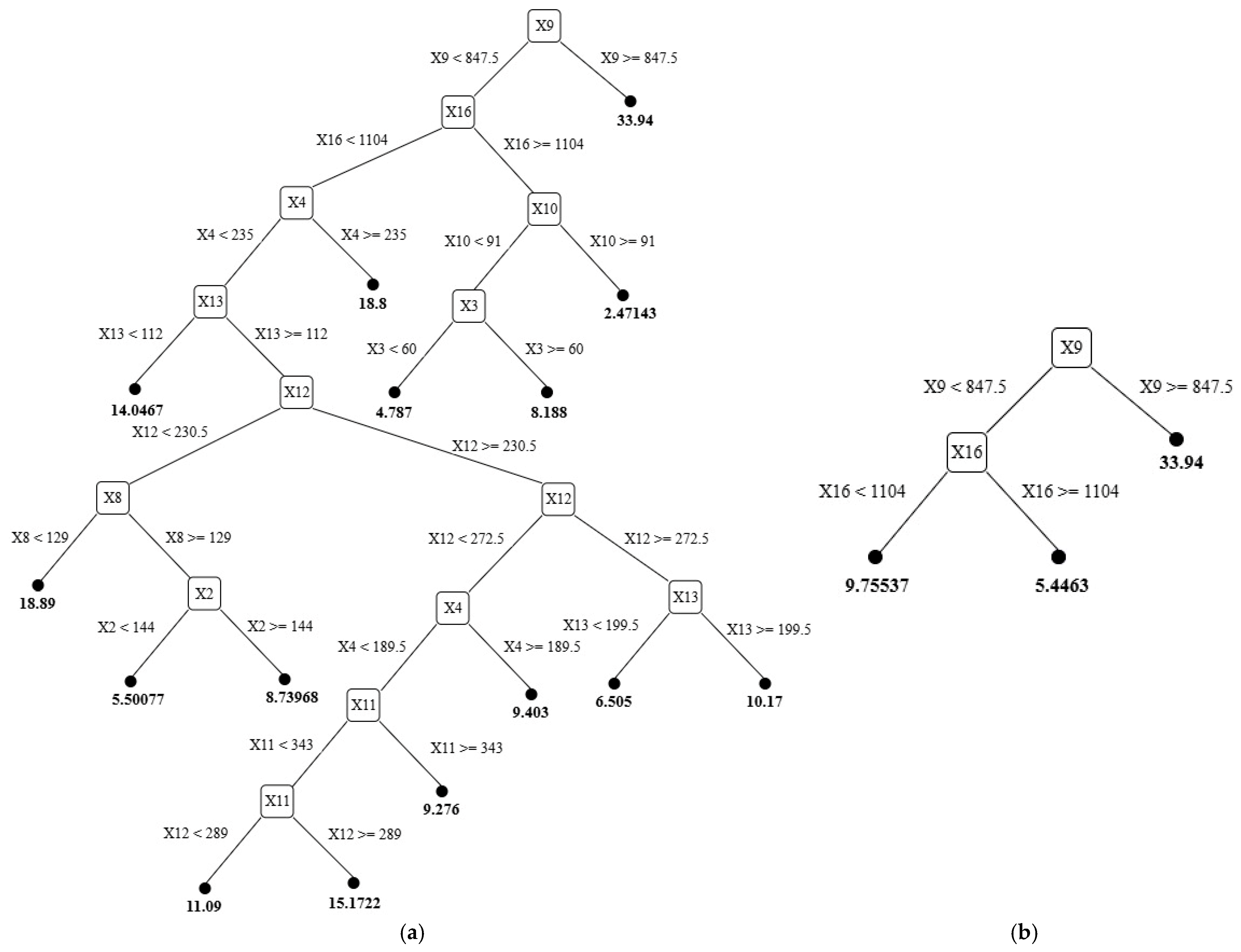
The pruned regression tree (Level 10) provides transparent decision-making pathways that can be directly interpreted in terms of soil moisture characteristics. Figure 7 compares the complete tree structure before and after pruning, demonstrating how the optimization process simplified the complex original tree (Figure 7a) into three essential decision pathways (Figure 7b), while preserving prediction accuracy.
The pruning process at Level 10 reduced the tree structure to only three essential leaf nodes, utilizing just two variables (X9 and X16), which demonstrates the model’s capability to avoid overfitting while maintaining predictive accuracy. The pruned tree structure reveals three primary decision pathways.
  • Decision Pathway 1
When X9 ≥ 847.5, the model directs to the right branch of the root node, leading to leaf node 3 with a predicted moisture content of 33.94%. This decision rule effectively identifies inland clayey soil sites where moisture retention is highest due to clay particles’ high specific surface area and low hydraulic conductivity.
  • Decision Pathway 2
When X9 < 847.5 AND X16 ≥ 1104, the model proceeds through node 2 to leaf node 5, predicting a low soil moisture content of 5.4463%. This pathway captures coastal sandy sites where rapid drainage and high hydraulic conductivity result in consistently low moisture levels.
  • Decision Pathway 3
When X9 < 847.5 AND X16 < 1104, the model predicts a moderate soil moisture content of 9.75537%. The pruning process simplified this pathway by removing node 4 and its subsequent branches, converting it directly to a leaf node to prevent overfitting while maintaining prediction accuracy. This pathway captures mixed alluvial deposits where intermediate moisture retention characteristics result from combined sandy and clayey compositions with moderate hydraulic conductivity.
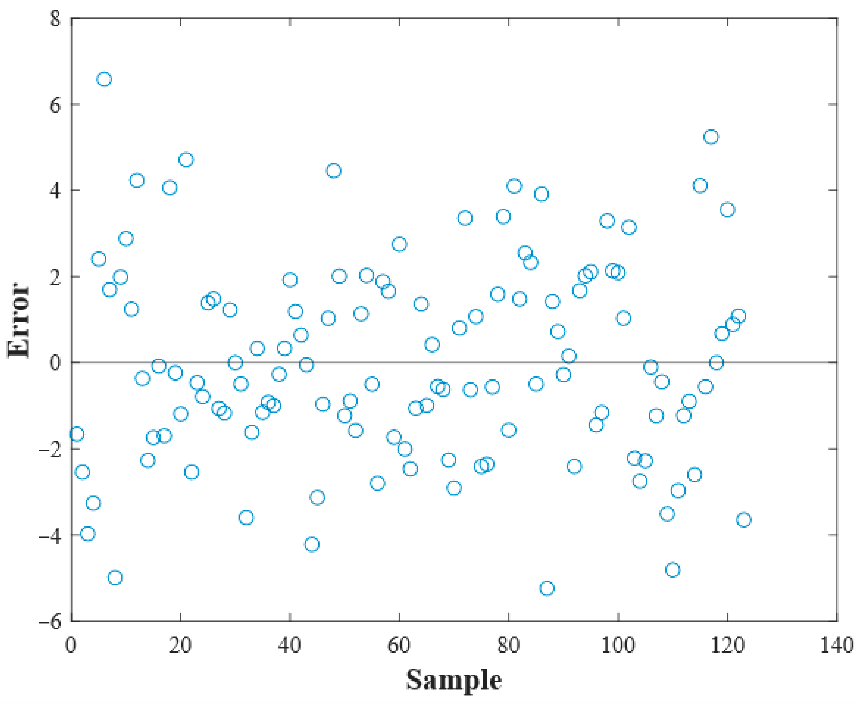
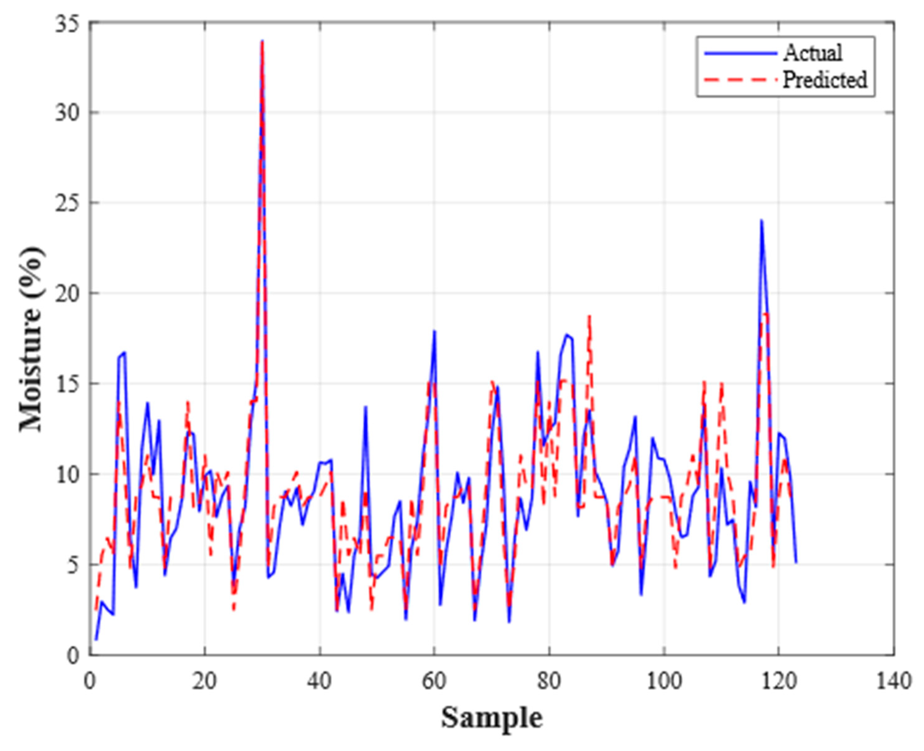
Figure 8 shows a residual plot for the pruned regression tree (Level 10), giving the distribution of prediction errors across all samples. Figure 9 presents a comparison between actual and predicted values using the optimized pruned regression tree, demonstrating the model’s prediction accuracy.

4.2.2. Boosted Tree Ensemble Optimization

Table 4 presents the maximum number of split optimization results for boosted tree ensembles, determining optimal configuration as a maximum of 3 splits with cross-validation RMSE = 4.818.
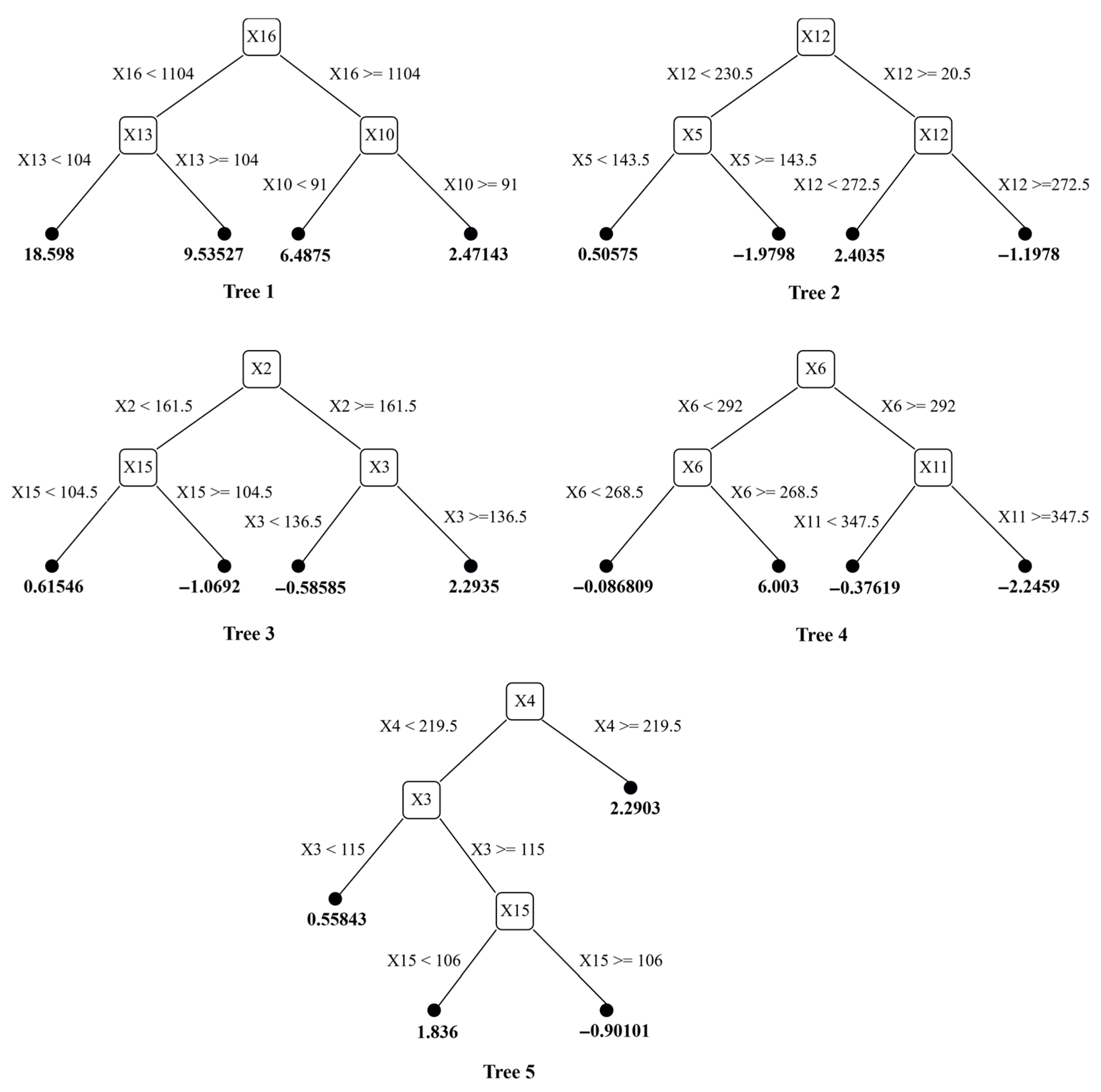
The configuration with a maximum of three splits was selected as optimal because it provided the best balance between training performance and generalization capability. While higher split numbers achieved better training metrics, they showed deteriorating cross-validation performance, indicating overfitting. Figure 10 illustrates the structure of all five trees in the refined ensemble, demonstrating the distributed decision-making process.
Unlike the single tree’s centralized decision structure, the boosted ensemble distributes the decision-making across multiple trees, each contributing to the final prediction through sequential error correction. The ensemble architecture demonstrates several key characteristics.
  • Distributed Feature Utilization
The five trees collectively utilize diverse histogram features (X16, X13, X10, X2, X12, X6, X3, X15, and others), enabling the ensemble to capture multidimensional relationships in the GPR data. This feature diversity allows the model to learn complex patterns that would be impossible for a single tree to capture.
  • Sequential Error Correction
Tree 1 provides an initial prediction based on X16 ≥ 1104, establishing the primary moisture classification. Trees 2–5 progressively refine this prediction by learning from the residual errors of previous iterations, with each tree focusing on different aspects of the feature space (X12, X6, X11, and X3).
  • Hierarchical Complexity Management
Each tree maintains simplicity (a maximum of three splits) to prevent overfitting, while the ensemble achieves complexity through the combination of multiple simple models. This approach balances predictive power and model stability.
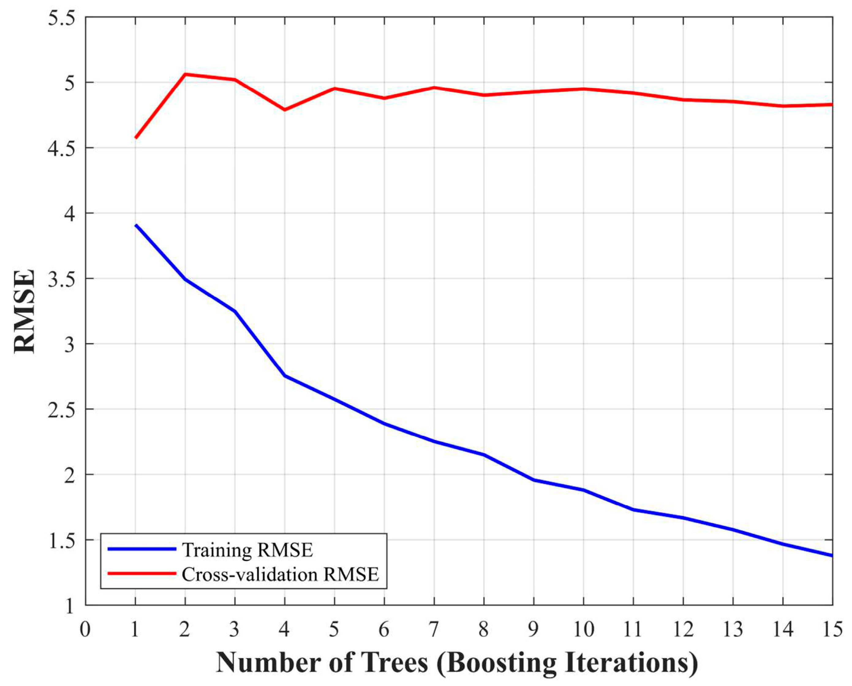
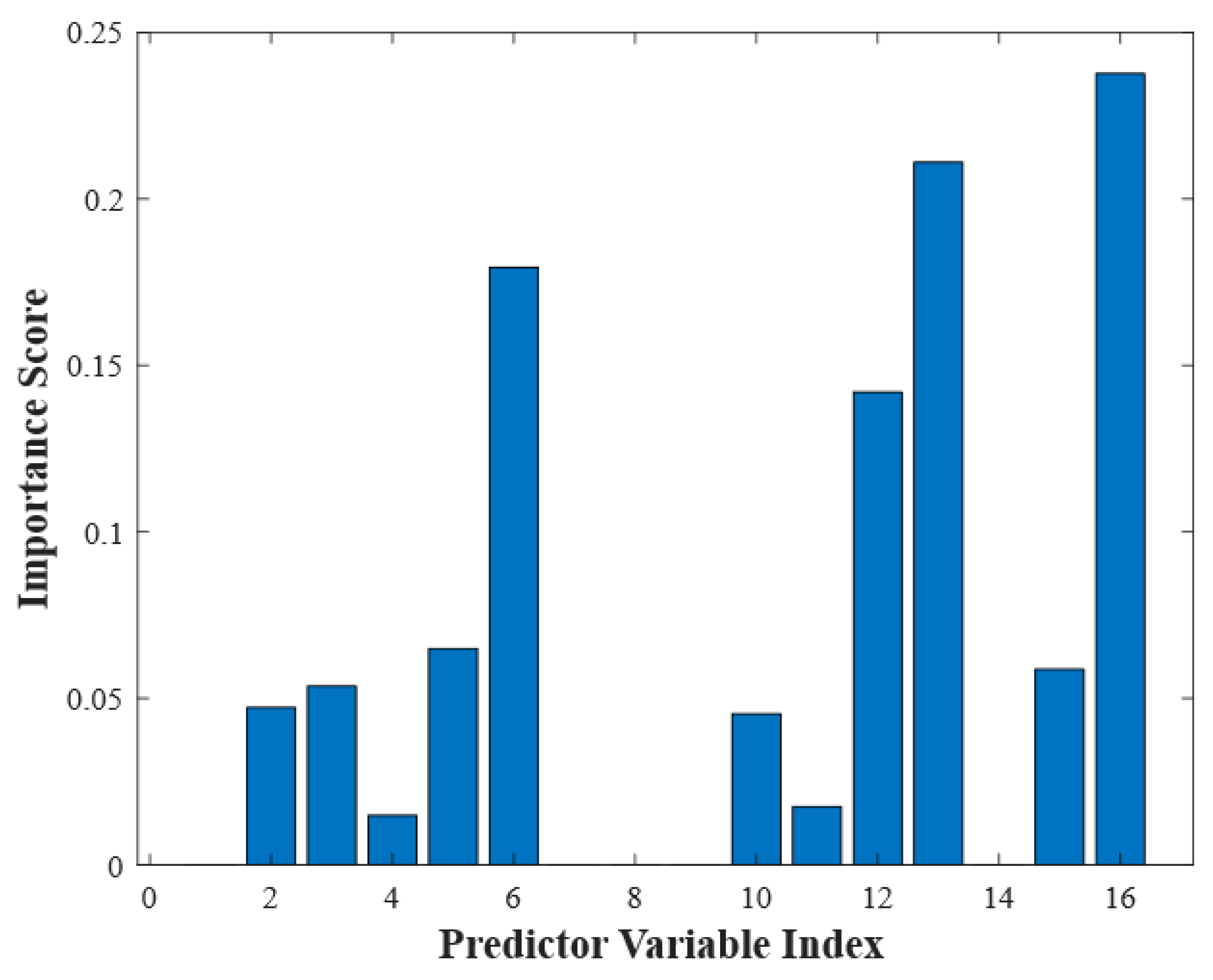
Figure 11 illustrates the learning curve of the boosted tree ensemble, showing both training and cross-validation RMSE versus the number of learning cycles. Figure 12 presents the relative importance scores across the 16-bin histogram, identifying which bins are most influential in the boosted ensemble’s prediction accuracy.
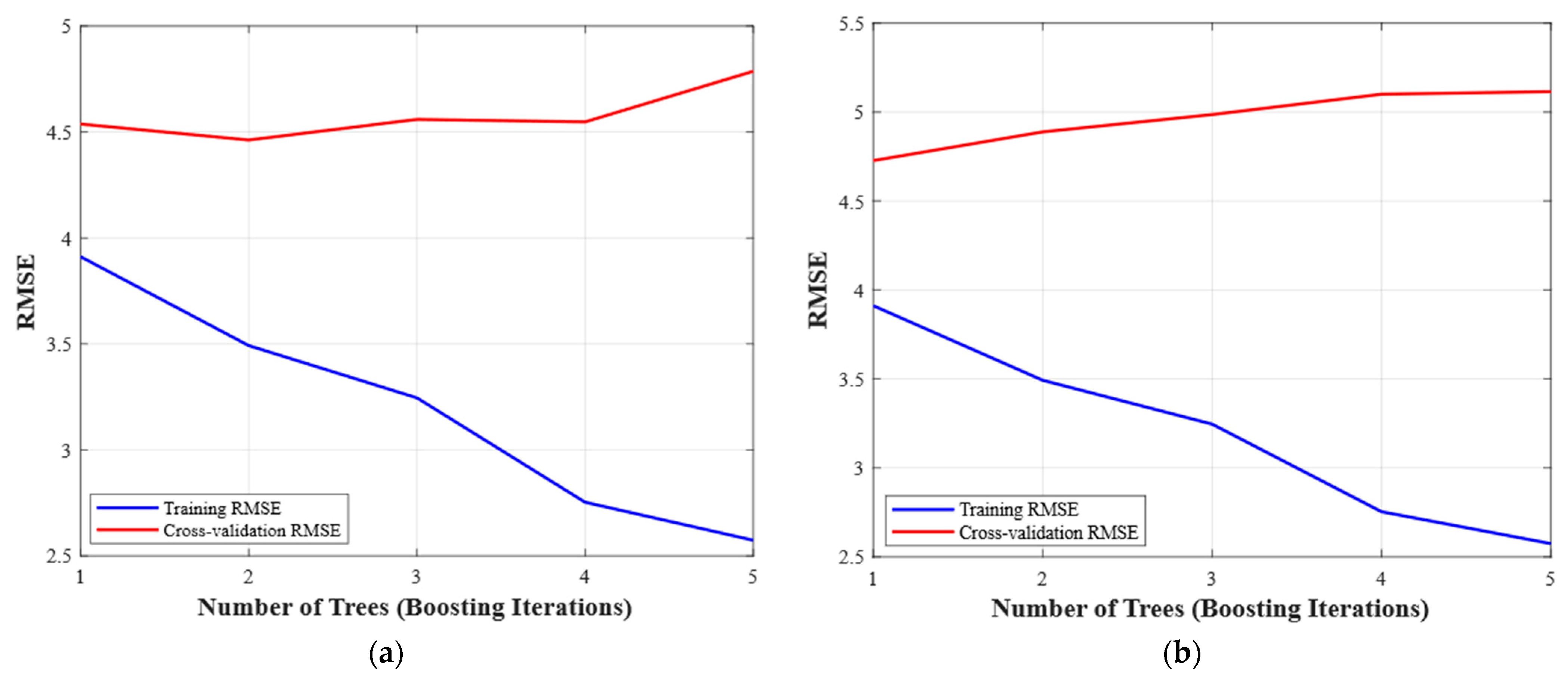
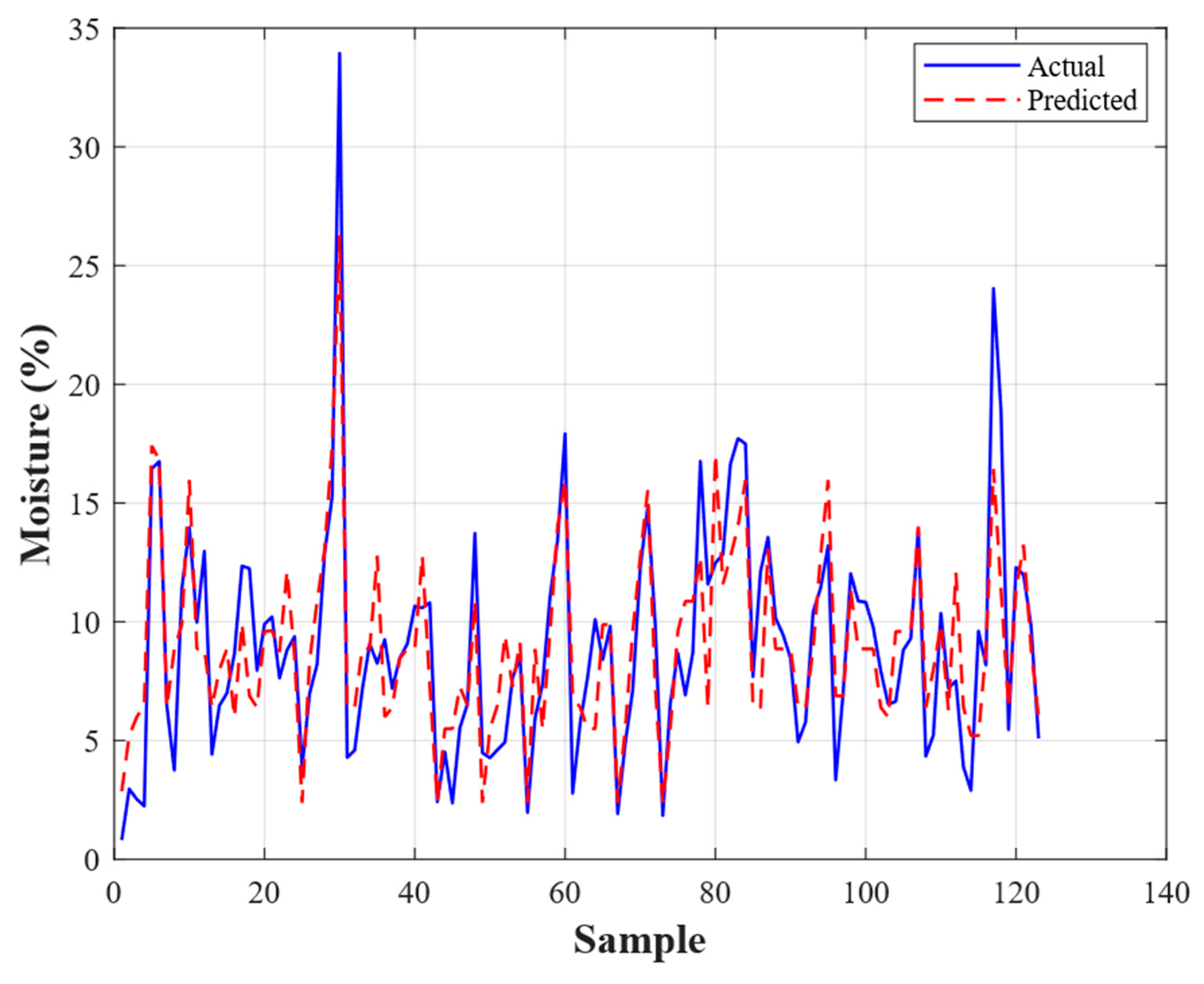
Figure 13 compares learning curves of (a) the original boosted tree ensemble, and (b) the refined model after feature selection. Figure 14 shows a residual plot of the refined boosted tree model, while Figure 15 presents a comparison of actual and predicted values using the refined model.

4.3. Comparative Performance Analysis

4.3.1. Overall Performance Comparison

Table 5 presents a systematic comparison of an optimized single regression tree and a boosted tree ensemble, revealing fundamental trade-offs that define these algorithmic approaches. The boosted tree ensemble demonstrated superior generalization performance, representing the most critical metric for real-world applications. However, the refined model showed reduced training accuracy, reflecting the classical bias-variance trade-off where ensemble methods achieve better generalization through sequential error correction at the cost of reduced training performance.

4.3.2. Performance Analysis by Soil Category

The analysis was carried out separately in each category to address the imbalance in the distribution of sites among soil categories (8 sites in coastal sandy and transitional mixed soils, 5 in inland clayey soils). A comparative evaluation of pruning Level 3 regression trees and the refined model on coastal sandy, transitional mixed, and inland clayey soils is presented in Table 6.
Of the three categories, transitional mixed soils revealed the greatest benefits of the enhanced ensemble, showing high training (R2 = 0.868 vs. 0.618) and generalization accuracy over the Level 3 tree (CV-RMSE = 4.644 vs. 4.556). The significant training enhancement shows that the ensemble error reduction is particularly effective with complex moisture patterns typical of mixed alluvial deposits. The validation-error reduction was the largest in inland clayey soils, although the sample size was smaller. The refined model had the lowest cross-validation error in all categories (CV-RMSE = 4.315 vs. 5.300), which further highlights the advantages of ensemble methods even when the training data is limited in soils with high moisture retention.

4.3.3. Algorithm Trade-Off Analysis

Comparative analysis reveals fundamental trade-offs between algorithmic approaches with important implications for practical deployment. The single regression tree has the advantage of interpretability, with easy-to-understand rules in the form of “if-then” statements that can be compared against known soil physics principles. The decision architecture of the single regression tree, defined by the X9 and X16 thresholds, gives a three-pathway decision architecture that is transparent in its reasoning to both researchers and practitioners.
In contrast, the enhanced ensemble achieves better predictive performance, but is effective only when an understanding of the entire ensemble of five interrelated trees is achieved. Thus, its interpretation is considerably more complex. Despite this complexity, the cross-validation improvements of the ensemble (5.7% improvement) indicate better generalization capability, a trend that is maintained across the three soil types (coastal sandy, transitional mixed, and inland clayey). The features of the ensemble are robust despite a skewed site distribution.
In terms of computational resource demands, the single tree is resource-light and can make predictions in real-time, which makes it applicable to field deployments. However, the ensemble has higher computational demands and produces more reliable predictions, which is a prudent trade-off when accuracy is the highest priority. The overall improvement in performance demonstrated by all categories of soil under analysis shows that the benefits of the enhanced ensemble are not limited to specific geological settings and support the overall validity of the comparative results.

4.4. Statistical Uncertainty Assessment

Statistical approaches to uncertainty evaluation were used to determine the reliability of comparative results and provide a strict validation of performance forecasts. A 5-fold cross-validation was performed 1000 times on each algorithm, with the same training data and hyperparameters used in all repetitions. This procedure was employed to isolate evaluation variance due to random fold allocation, which is a significant source of uncertainty in cross-validation, and hence increases confidence in results.
Since the accuracy of generalization, rather than training performance, is the critical dimension of model robustness, cross-validation RMSE was chosen as the main measure of uncertainty. The other performance measures, R2, training RMSE, and MAE, were also constant across iterations because both algorithms are deterministic when used with the same datasets. The random division of the training data during cross-validation was the only factor that introduced variation, thus making cross-validation RMSE the best measure of performance uncertainty and of the relative stability of the two modeling strategies.
The uncertainty analysis based on 1000 replications revealed statistically significant performance differences between algorithms. The non-overlapping confidence intervals (Table 7) provide strong statistical evidence for the superior generalization capability of boosted tree ensembles, confirming the reliability of comparative results across diverse soil conditions.
The variability of the models was also evaluated using the coefficient of variation. A single regression tree was more sensitive to the composition of the folds, but the boosted ensemble was more consistent across folds. This finding supports theoretical predictions of ensembles, which integrate several weak elements to reduce variability in performance. As a result, the enhanced ensemble provides more reliable forecasts at operational locations, where continuity between different soil areas is critical.
The uncertainty analysis using the repetitions resulted in outcomes that were slightly different from those achieved in the single deterministic analysis reported in Table 5. The single regression tree had a 5.082 cross-validation RMSE while the boosted ensemble had 4.7915. The magnitude of improvement (8.6% in repeated analysis vs. 5.7% in single analysis) and ranking are the same across evaluation methods. The narrow, non-overlapping confidence intervals provide strong statistical evidence for the performance difference between the two methods. The lack of overlap confirms that the observed performance difference is statistically significant rather than due to random variation, giving high confidence in the relative ranking of the models.

5. Discussion

5.1. Key Research Findings

This systematic comparison confirms the superior generalization capability of boosted tree ensembles, with statistically significant performance improvements detailed in the comparative analysis (Section 4.3). However, single regression trees have better interpretability of the model with clear decision rules. The single regression tree achieved optimal performance at pruning level 10 with superior training accuracy (Table 3). Table 4 shows the boosted ensemble’s optimal configuration with a maximum of 3 splits. The ensemble performs better due to the capability of weak learners to correct errors through the boosting process [19], as illustrated in the learning curves shown in Figure 11.
The moisture-related variations in the GPR distribution of signal amplitudes were effectively captured by the histogram-based feature extraction technique. This is evidenced in Figure 5, where the bins with significantly different predictive accuracy of the results were identified. Figure 12 demonstrates the predictor importance analysis, revealing that specific histogram bins (particularly bins 6, 12, 13, and 16) contributed most significantly to model performance. The result of feature selection was a one-third reduction in the optimal feature set (16 variables down to nine), as shown in a comparison between Figure 13a,b. This enabled improvement of the computational efficiency while retaining similar predictive performance. The residual plots (Figure 8 and Figure 14) demonstrate improved error distribution in the refined boosted model compared to the single regression tree.

5.2. Comparison with Previous Research

The current results align with previous research demonstrating ensemble method superiority in soil moisture estimation (R2 = 0.79) [11]. Our boosted ensemble achieved R2 = 0.708 with superior cross-validation performance, confirming theoretical ensemble advantages [19]. The 5.7% cross-validation RMSE improvement confirms practical benefits for GPR applications. The predictor importance analysis aligns with previous findings on ensemble method superiority in geophysical applications [20].
The histogram-based feature extraction approach is consistent with recent work on GPR histogram percentiles contributing to model accuracy [25]. A 16-bin histogram approach represents development of frequency-domain processes [6] and envelope detection methods [27]. The learning curves presented in Figure 11 and Figure 13 demonstrate convergence behavior that extends previous research on ensemble algorithm evaluation. Recent studies have demonstrated the feasibility of using digital image color data with machine learning algorithms to rapidly estimate soil water content, offering vision-based alternatives to sensor-based approaches [34].
The comparative framework constructed here addresses existing gaps [29,30,31,32,33] and provides a systematic evaluation absent in the literature. It was developed based on established tree-based evaluation methods [17] and ensemble approaches [18]. The performance comparison results (Table 5) and systematic optimization approach (Table 1 and Table 3) supplement current GPR applications in infrastructure surveillance and geotechnical evaluation, while broadening operational capacity in pavement and foundation engineering conditions.

5.3. Engineering Applications and Practical Implementation

For operational applications in real-time precision agriculture and irrigation management, the results indicate that boosted tree ensembles are preferred. The 5.7% RMSE improvement demonstrated in Table 5 translates to enhanced moisture predictions, with potential irrigation efficiency improvements of 15–20%. The residual plots (Figure 8 vs. Figure 14) show more consistent error distribution in the boosted ensemble, critical for reliable field applications.
Single regression trees are beneficial in research and development situations, as evidenced by their higher training R2 (0.761 vs. 0.708, Table 5) and interpretable decision rules. The computational overhead analysis reveals that boosted ensembles require approximately five times the processing time, as indicated by the convergence patterns in the learning curves (Figure 11). However, this is justified in high-stakes applications where prediction accuracy is paramount.
The diverse soil conditions tested (Table 2)—ranging from coastal sandy soils (6.96–14.80% moisture) to inland clays (5.85–21.28% moisture)—validate the generalizability of the comparative framework across Thailand’s varied geological conditions for precision agriculture applications.

5.4. Study Limitations

The limitations of the methodology are as follows. The work is limited to feature extraction using histograms, but alternative methods, like frequency-domain analysis [6], envelope detection [27], spectral features [26], and AEA methods [7,8], may provide different comparative results that could be used to identify more suitable analytical algorithms. The histogram specification used a fixed 16-bin division, and an alternate number of bins could affect the performance characterizations and comparative merits of standalone and ensemble performance. Additionally, the study used GPR data with a single frequency of 500 MHz, thereby limiting direct correlation of the research results with other electromagnetic systems at frequencies outside this range [20,24]. Changes in soil properties induced by frequency can alter algorithm performance in different spectra, which limits generalizability to particular soil types and environmental conditions.
The geographical and environmental factors in the evaluations are also limited. The study was conducted in Eastern Thailand under tropical climate conditions. Validation is needed to confirm whether the framework can be applied to different climatic conditions to ensure its broader validity. The analyzed stratigraphy encompassed sandy and clayey deposits of coastal and inland areas, thus limiting its applicability to these geological conditions with distinct electromagnetic and water-retention features. Seasonal fluctuations were ignored. Thus, single-period data acquisition could not represent the impacts of seasonal fluctuations on the dynamics of soil moisture over time [1]. Accordingly, measurement consistency of performance is questionable over time.
Additional interpretive difficulties arise due to data collection limitations. A total of 123 out of the 126 planned samples were collected, resulting in an uneven sample distribution amongst the different soil types, which could affect training accuracy and balance. Sampling was extended from 0.5 m to 3.0 m, but deeper moisture measurements needed in some applications were not sampled. Additionally, unavailable data in three Standard Penetration Test (SPT) instances also weakened the statistical power set to make some soil comparisons and lowered the representativeness of the final dataset.
The generalizability of conclusions is also limited by algorithmic constraints. Only two tree-based methods were compared. Other machine learning architectures, neural networks [13], support vector machines, hybrid ensembles [15], and deep learning models [28] could produce different accuracy-interpretability trade-offs. The predictor importance analysis was based on the scores of predictors as opposed to the full sensitivity analysis [14,15], which could mask the intricacies of the feature interactions and their effect on model performance. The hyperparameter space was sparsely sampled due to computational limitations. Furthermore, parameter selection might have been sub-optimal. Additional optimization runs might produce finer performance boundaries [29,30,31,32,33], indicating that apparent advantages may be partially due to an inferior choice of parameters rather than inherent superiority of algorithms.

6. Conclusions

This systematic evaluation assessed single regression trees versus boosted tree ensembles for GPR-based soil moisture prediction using 16-bin histogram features from 21 sites across Eastern Thailand, revealing fundamental insights for algorithm selection in geotechnical and precision agriculture applications.
  • Superior Ensemble Performance: Boosted tree ensembles achieved statistically significant generalization improvements with cross-validation RMSE of 4.7915 compared to 5.082 for single trees (5.7% improvement), confirmed through a 1000-iteration uncertainty analysis;
  • Interpretability Trade-offs: Single regression trees provided transparent three-pathway decision structures utilizing only two histogram features, enabling direct validation against soil physics principles, while ensemble methods required understanding of five interrelated trees;
  • Robust Cross-Condition Performance: Ensemble advantages were consistent across all soil categories, with the most significant improvements in transitional mixed soils (R2 = 0.868 vs. 0.618).
  • Effective Feature Extraction: 16-bin histogram configuration optimally balanced training accuracy and generalization capability, with specific bins (6, 12, 14, and 16) contributing most significantly to prediction performance.
For operational applications, boosted tree ensembles are recommended for precision irrigation systems where prediction accuracy drives economic value, with 5.7% RMSE improvement translating to potential irrigation efficiency gains of 15–20%. Single regression trees are preferred for research applications where interpretability facilitates scientific validation. The methodology’s effectiveness across diverse geological conditions validates its applicability for Southeast Asian contexts.
Future research should prioritize multi-frequency GPR integration, complementary sensing fusion with thermal imaging and UAV-derived data, and climate adaptation studies extending framework validation beyond tropical conditions. The methodology provides a robust foundation for advancing non-destructive soil characterization technologies, enabling practitioners to make informed algorithmic choices based on specific application requirements.

Author Contributions

Conceptualization, J.P. and S.E.-a.; methodology, J.P. and S.E.-a.; software, J.P.; validation, J.P., P.H., R.A. and S.E.-a.; formal analysis, J.P. and S.E.-a.; investigation, P.H. and R.A.; resources, S.E.-a.; data curation, S.E.-a.; writing—original draft preparation, S.E.-a.; writing—review and editing, J.P., P.H., R.A. and S.E.-a.; visualization, J.P., R.A. and S.E.-a.; supervision, J.P. and S.E.-a. All authors have read and agreed to the published version of the manuscript.

Funding

This research received no external funding.

Data Availability Statement

The datasets generated during this study are available from the corresponding author upon reasonable request. Access to raw GPR data may require appropriate data use agreements due to the sensitive nature of infrastructure site information.

Conflicts of Interest

The authors declare no conflicts of interest.

References

  1. Iwasaki, K.; Tamura, M.; Sato, H.; Masaka, K.; Oka, D.; Yamakawa, Y.; Kosugi, K. Application of Ground-Penetrating Radar and a Combined Penetrometer–Moisture Probe for Evaluating Spatial Distribution of Soil Moisture and Soil Hardness in Coastal and Inland Windbreaks. Geosciences 2020, 10, 238. [Google Scholar] [CrossRef]
  2. Davis, J.L.; Annan, A.P. Ground-penetrating radar for high-resolution mapping of soil and rock stratigraphy. Geophys. Prospect. 1989, 37, 531–551. [Google Scholar] [CrossRef]
  3. Topp, G.C.; Davis, J.L.; Annan, A.P. Electromagnetic determination of soil water content: Measurements in coaxial transmission lines. Water Resour. Res. 1980, 16, 574–582. [Google Scholar] [CrossRef]
  4. Huisman, J.A.; Hubbard, S.S.; Redman, J.D.; Annan, A.P. Measuring soil water content with ground penetrating radar: A review. Vadose Zone J. 2003, 2, 476–491. [Google Scholar] [CrossRef]
  5. Van Dam, R.L. Calibration functions for estimating soil moisture from GPR dielectric constant measurements. Commun. Soil Sci. Plant Anal. 2014, 45, 392–413. [Google Scholar] [CrossRef]
  6. Benedetto, A. Water content evaluation in unsaturated soil using GPR signal analysis in the frequency domain. J. Appl. Geophys. 2010, 71, 26–35. [Google Scholar] [CrossRef]
  7. Liu, K.; Lu, Q.; Zeng, Z.; Li, Z. Estimation of soil moisture content of farmlands based on AEA method of GPR. J. Phys. Conf. Ser. 2023, 2651, 12036. [Google Scholar] [CrossRef]
  8. Mesquita, M.J.L.; Luiz, J.G.; da Costa, J.P.R. Estimates of soil water content using ground penetrating radar in field conditions. Rev. Bras. Geofís. 2015, 33, 389–401. [Google Scholar] [CrossRef]
  9. Li, K.; Liao, Z.; Ji, G.; Zhang, D.; Liu, H.; Yang, X.; Zhang, S. Estimation of the Soil Moisture Content in a Desert Steppe on the Mongolian Plateau Based on Ground-Penetrating Radar. Sustainability 2024, 16, 8558. [Google Scholar] [CrossRef]
  10. Akinsunmade, A. Towards an Evaluation of Soil Structure Alteration from GPR Responses and Their Implications for Management Practices. Appl. Sci. 2025, 15, 6078. [Google Scholar] [CrossRef]
  11. Chen, L.; Xing, M.; He, B.; Wang, J.; Shang, J.; Huang, X.; Xu, M. Estimating soil moisture over winter wheat fields during growing season using machine-learning methods. IEEE J. Sel. Top. Appl. Earth Obs. Remote Sens. 2021, 14, 3706–3718. [Google Scholar] [CrossRef]
  12. Dabboor, M.; Atteia, G.; Alnashwan, R. Optimizing Soil Moisture Retrieval: Utilizing Compact Polarimetric Features with Advanced Machine Learning Techniques. Land 2023, 12, 1861. [Google Scholar] [CrossRef]
  13. Uthayakumar, A.; Mohan, M.P.; Khoo, E.H.; Jimeno, J.; Siyal, M.Y.; Karim, M.F. Machine learning models for enhanced estimation of soil moisture using wideband radar sensor. Sensors 2022, 22, 5810. [Google Scholar] [CrossRef] [PubMed]
  14. Qiao, X.; Yang, F.; Xu, X. The prediction method of soil moisture content based on multiple regression and RBF neural network. In Proceedings of the 15th International Conference on Ground Penetrating Radar, Brussels, Belgium, 30 June–4 July 2014; pp. 140–143. [Google Scholar]
  15. Liang, J.; Liu, X.; Liao, K. Soil moisture retrieval using UWB echoes via fuzzy logic and machine learning. IEEE Internet Things J. 2015, 2, 651–661. [Google Scholar] [CrossRef]
  16. Qiu, C.; Du, W.; Zhang, S.; Guo, W.; Liu, B.; Liu, Y. Shallow Subsurface Soil Moisture Estimation in Coal Mining Area Using GPR Signal Features and BP Neural Network. Water 2025, 17, 873. [Google Scholar] [CrossRef]
  17. Breiman, L. Random Forests. Mach. Learn. 2001, 45, 5–32. [Google Scholar] [CrossRef]
  18. Freund, Y.; Schapire, R.E. A decision-theoretic generalization of on-line learning and an application to boosting. J. Comput. Syst. Sci. 1997, 55, 119–139. [Google Scholar] [CrossRef]
  19. Friedman, J.H. Greedy function approximation: A gradient boosting machine. Ann. Stat. 2001, 29, 1189–1232. [Google Scholar] [CrossRef]
  20. Pathirana, S.; Lambot, S.; Krishnapillai, M.; Cheema, M.; Smeaton, C.; Galagedara, L. Integrated ground-penetrating radar and electromagnetic induction offer a non-destructive approach to predict soil bulk density in boreal podzolic soil. Geoderma 2024, 450, 117028. [Google Scholar] [CrossRef]
  21. Nduku, L.; Munghemezulu, C.; Mashaba-Munghemezulu, Z.; Malobola, N. Field-Scale Winter Wheat Growth Prediction Applying Machine Learning Methods with UAV Imagery and Soil Properties. Land 2024, 13, 299. [Google Scholar] [CrossRef]
  22. Atun, R.; Gürsoy, Ö.; Koşaroğlu, S. Field Scale Soil Moisture Estimation with Ground Penetrating Radar and Sentinel 1 Data. Sustainability 2024, 16, 10995. [Google Scholar] [CrossRef]
  23. Papadopoulos, A.; Apostolopoulos, G.; Kofakis, P.; Gonos, I.F.; Tsokas, G.N.; Tsourlos, P.I.; Soupios, P.M. A Combined Hydrogeophysical System for Soil Column Experiments Using Time Domain Reflectometry and Ground-Penetrating Radar. Water 2025, 17, 2003. [Google Scholar] [CrossRef]
  24. Zhao, S.; Al-Qadi, I.L. Algorithm development for real-time thin asphalt concrete overlay compaction monitoring using ground-penetrating radar. NDT E Int. 2019, 104, 114–123. [Google Scholar] [CrossRef]
  25. Vahidi, M.; Shafian, S.; Frame, W.H. Multi-modal sensing for soil moisture mapping: Integrating drone-based ground penetrating radar and RGB-thermal imaging with deep learning. Comput. Electron. Agric. 2025, 236, 110423. [Google Scholar] [CrossRef]
  26. Haghniaz Jahromi, V.; Filardi, S.; Zekavat, Z.; Wang, J.; Thurber, D.; Hoffman, C.; Larson, R.; Petkie, D. Toward intelligent adaptive airborne GPR, implementation and data acquisition. In Proceedings of the 2024 IEEE International Conference on Wireless for Space and Extreme Environments (WiSEE), Seoul, Republic of Korea, 19–21 August 2024; pp. 253–258. [Google Scholar]
  27. He, Y.; Fang, L.; Peng, S.; Liu, W.; Cui, C. A ground-penetrating radar-based study of the structure and moisture content of complex reconfigured soils. Water 2024, 16, 2332. [Google Scholar] [CrossRef]
  28. Alzubaidi, L.; Chlaib, H.K.; Fadhel, M.A.; Chen, Y.; Bai, J.; Albahri, A.S.; Gu, Y. Reliable deep learning framework for the ground penetrating radar data to locate the horizontal variation in levee soil compaction. Eng. Appl. Artif. Intell. 2024, 129, 107627. [Google Scholar] [CrossRef]
  29. Riese, F.M.; Keller, S. Fusion of hyperspectral and ground penetrating radar data to estimate soil moisture. In Proceedings of the 2018 9th Workshop on Hyperspectral Image and Signal Processing: Evolution in Remote Sensing (WHISPERS), Amsterdam, The Netherlands, 23–26 September 2018; pp. 1–5. [Google Scholar]
  30. Wang, P.; Hu, Z.; Zhao, Y.; Li, X. Experimental study of soil compaction effects on GPR signals. J. Appl. Geophys. 2016, 126, 128–137. [Google Scholar] [CrossRef]
  31. Anbazhagan, P.; Chandran, D.; Burman, S. Investigation of soil compaction homogeneity in a finished building using ground penetrating radar. In Proceedings of the Forensic Engineering 2012, ASCE, San Francisco, CA, USA, 31 October–3 November 2012; pp. 773–782. [Google Scholar]
  32. Leng, Z.; Al-Qadi, I.L.; Lahouar, S. Development and validation for in situ asphalt mixture density prediction models. NDT E Int. 2011, 44, 369–375. [Google Scholar] [CrossRef]
  33. Plati, C.; Georgiou, P.; Loizos, A. A comprehensive approach for the assessment of HMA compactability using GPR technique. Near Surf. Geophys. 2016, 14, 117–126. [Google Scholar] [CrossRef]
  34. Liu, G.; Tian, S.; Xu, G.; Zhang, C.; Cai, M. Combination of effective color information and machine learning for rapid prediction of soil water content. J. Rock Mech. Geotech. Eng. 2023, 15, 2441–2457. [Google Scholar] [CrossRef]
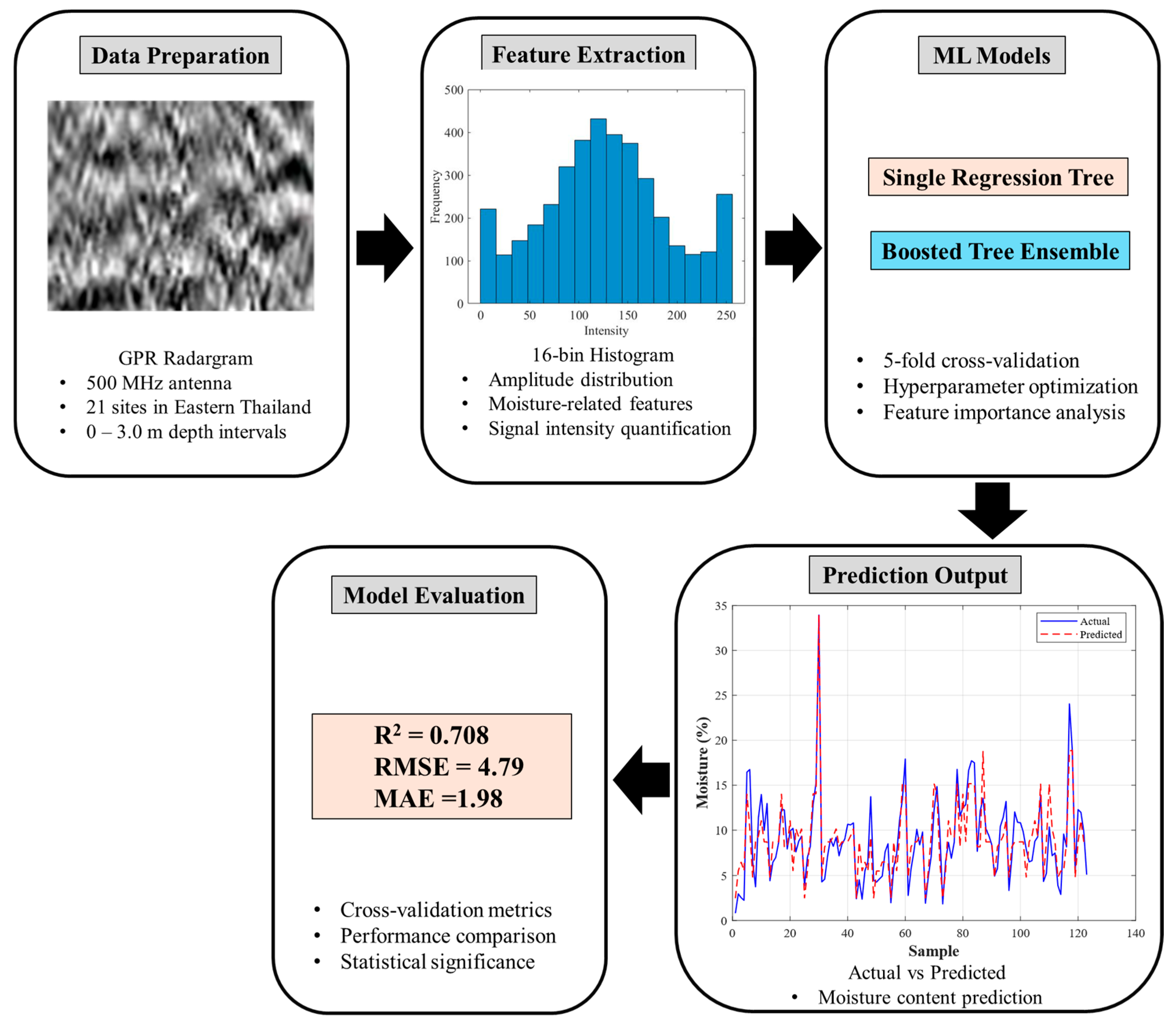
Figure 1. Framework overview for soil moisture prediction using GPR.
Earth 06 00098 g001
Figure 2. Location of 21 test sites in Rayong and Chonburi provinces, Eastern Thailand. (a) Location map of the study area within Thailand. (b) Detailed study area showing site distribution across coastal and inland regions.
Earth 06 00098 g002
Figure 3. Field Data Collection (a) MALA Easy Locator GPR system operation during field data collection, and (b) Standard Penetration Test (SPT) sampling procedure at the test sites.
Earth 06 00098 g003
Figure 4. Example of GPR images from locations 1, 10, and 20 with multiple depth intervals.
Earth 06 00098 g004
Figure 5. Examples of the resulting histograms corresponding to the GPR images at multiple depths.
Earth 06 00098 g005
Figure 6. Flowchart of the Boosted Tree Ensemble (Refined Model).
Earth 06 00098 g006
Figure 7. Regression Tree Structure showing (a) complete tree before pruning, and (b) optimized Level 10 pruned tree with three decision pathways.
Earth 06 00098 g007
Figure 8. Residual plot of the Pruned Regression Tree (Level 10) showing the distribution of prediction errors.
Earth 06 00098 g008
Figure 9. Comparison of actual and predicted values using a Pruned Regression Tree (Level 10).
Earth 06 00098 g009
Figure 10. Boosted Tree Ensemble Structure showing five sequential trees (Trees 1–5) with a maximum of 3 splits.
Earth 06 00098 g010
Figure 11. A Learning Curve of Boosted Tree Ensemble showing training and cross-validation RMSE versus the number of learning cycles.
Earth 06 00098 g011
Figure 12. Predictor Importance of a Boosted Tree Ensemble showing relative importance scores for histogram features.
Earth 06 00098 g012
Figure 13. Learning Curve comparison of (a) a Boosted Tree Ensemble, and (b) a Refined Model after feature selection.
Earth 06 00098 g013
Figure 14. Residual plot of a Refined Boosted Tree Model.
Earth 06 00098 g014
Figure 15. Comparison of Actual and Predicted Values using a Refined Boosted Tree Model.
Earth 06 00098 g015
Table 1. Performance Comparison Across Different Histogram Bin Sizes.
Bin SizeSingle Regression Tree (Level 10)Boosted Tree Ensemble (Refined Model)
R2RMSEMAECV-RMSER2RMSEMAECV-RMSE
4-bin0.3953.7072.8346.0360.5103.3372.5474.772
8-bin0.7022.6011.8215.8410.6072.9882.3024.632
12-bin0.6832.6812.0535.4150.6542.8042.0694.785
16-bin0.7612.3301.9015.0820.7082.5741.9824.792
20-bin0.6642.7622.0505.5570.6672.7502.1975.079
24-bin0.7782.2451.8245.7040.7342.4571.8535.224
Table 2. Summary of Geological Conditions at Test Sites.
Site
Category
Number of SitesDominant Soil TypesNatural Water Content Range (%)SPT N-Value Range (Blows/ft)Geological Characteristics
Coastal Sandy8Poorly graded sands (SP), silty sands (SM)6.96–14.806–62Well-drained coastal deposits, low plasticity, variable density
Transitional Mixed8Silty sands (SM)5.74–13.526–53Mixed alluvial deposits, moderate moisture retention, dense
Inland Clayey5Low plasticity clays (CL), clayey sands (SP-CL)5.85–21.289–62Fine-grained soils, high moisture retention, plastic behavior
Table 3. Model Performance across Various Pruning Levels for a Single Regression Tree.
Performance MetricLevel
468101214
R20.8350.8220.7850.7610.7260.657
RMSE1.9362.0122.2122.3302.4962.790
MAE1.5081.5991.7911.9011.9922.209
RMSE
cross-validation (K = 5)
5.3545.4755.8355.0825.2995.618
Table 4. Maximum Number of Splits Optimized for a Boosted Tree Ensemble.
Performance MetricMaximum Number of Splits
13579111315
R20.3990.7080.8290.8560.9070.9300.9570.963
RMSE3.6952.5741.9681.8111.4501.2590.9940.917
MAE2.8011.9821.5061.3841.1660.9460.7330.637
RMSE
cross-validation (K = 5)
4.7374.8185.2835.1685.5915.2705.4235.164
Table 5. Comparison of a Pruned Regression Tree and Boosted Tree Ensemble (Refined Model).
Performance MatricesPruned Regression TreeBoosted Tree Ensemble (Refined Model)
R20.7610.708
RMSE2.3302.574
MAE1.9011.982
RMSE
cross-validation (K = 5)
5.0824.7915
Table 6. Model Performance by Soil Category.
Soil CategoryAlgorithmR2RMSEMAECV-RMSE
Coastal SandySigle Tree (Pruned Level 3)0.8322.1771.6865.923
(8 sites)Boosted Tree (Refined)0.9061.6321.2656.081
Transitional MixedSigle Tree (Pruned Level 3)0.6182.6472.1624.556
(8 sites)Boosted Tree (Refined)0.8681.5531.2204.644
Inland ClayeySigle Tree (Pruned Level 3)0.8801.5641.1715.300
(5 sites)Boosted Tree (Refined)0.9111.3491.0584.315
Note: Pruning Level 10 could not be applied to individual soil categories due to insufficient data; Level 3 pruning was used instead.
Table 7. Repeated Cross-Validation Uncertainty Analysis (1000 iterations).
AlgorithmMean
CV-RMSE
Standard
Deviation
95% Confidence
Interval
Coefficient of
Variation
Single Regression Tree
(Level 10)
5.45890.3374[5.4379, 5.4798]6.18%
Boosted Tree (Refined)4.98740.2596[4.9713, 5.0035]5.20%
Disclaimer/Publisher’s Note: The statements, opinions and data contained in all publications are solely those of the individual author(s) and contributor(s) and not of MDPI and/or the editor(s). MDPI and/or the editor(s) disclaim responsibility for any injury to people or property resulting from any ideas, methods, instructions or products referred to in the content.