Abstract
Land degradation in drylands represents a critical environmental challenge, with persistent bare soil serving as a key indicator of ecosystem vulnerability, including in the Caatinga biome. This study maps and analyzes the spatial and temporal dynamics of persistent bare soils over three decades using multi-temporal remote sensing data. We applied Spectral Mixture Analysis (SMA), temporal metrics, and machine learning classifiers within Google Earth Engine to process long-term Landsat datasets and to derive the Normalized Difference Fraction Index Adjusted (NDFIa). The results indicate a widespread increase in bare soil, with over 63% of mapped hexagons showing expansion, particularly in the São Francisco Basin. Peaks in soil exposure coincided with severe drought events, highlighting the link between climate variability and land degradation. Moreover, abandoned agricultural lands and pasturelands emerged as the dominant contributors to persistent bare soils. These findings reinforce the need for targeted policies to mitigate land degradation and to promote sustainable land management in semi-arid ecosystems. This research provides a robust framework for long-term environmental monitoring in drylands by integrating satellite data with advanced analytical techniques. These advancements support more effective land management and conservation strategies in semi-arid ecosystems.
1. Introduction
The spatial expansion of unproductive lands, reflected in the growth of bare soils highly susceptible to erosion, is a key indicator of land degradation in drylands [1,2]. These regions, which cover approximately 46.2% of the Earth’s surface and support over 3 billion people, are particularly susceptible to desertification processes and are significantly influenced by global climate change [1,3,4,5]. In the Caatinga biome, a seasonally dry tropical forest located in Brazil’s semi-arid Northeast, the occurrence and spread of bare soils result directly from deforestation and intensive land use without sustainable management [5,6], compounded by climate changes that have intensified and extended drought periods in the region [7].
In general, understanding land use and land cover dynamics and monitoring land degradation has relied heavily on remote sensing techniques [3,8,9]. Initially, studies were limited in temporal and spatial scales [10,11]. However, mainly since the 2010s, the continuous development of large-scale data generation, driven by advancements in computational power, such as cloud computing, more powerful hardware, and robust algorithms, has enabled broader and more detailed analyses [5,12,13,14,15]. Most of these studies have focused on monitoring tropical rainforest regions [16,17,18,19], where global attention has traditionally been directed.
Monitoring drylands with remote sensing remains challenging due to their unique environmental characteristics, such as low vegetation cover, variable rainfall, distinct climatic seasonality, and interference from clouds and shadows in satellite imagery [5,7,20,21]. These factors make it more difficult to detect land cover changes and accurately identify degradation indicators [6]. Mapping persistent bare soils, however, has long been recognized as a critical variable for assessing land degradation in drylands, particularly due to its association with vegetation loss, erosion susceptibility, and reduced soil productivity [1,21,22,23,24]. In these environments, where climatic seasonality and anthropogenic pressure intersect, soil exposure often results from unsustainable agriculture, non-managed pasture, deforestation, or climatic shocks such as prolonged droughts [22,25].
Such bare soil exposure reflects a loss of ecosystem resistance and may precede a decline in recovery capacity, particularly when disturbances are recurrent or compounded by anthropogenic pressures [23]. Remote sensing approaches have proven effective in capturing the spatial and temporal patterns of bare soil distribution, enabling the detection and monitoring of degradation patterns in rangeland ecosystems [1,22,23,25]. Nonetheless, mapping persistent bare soils is essential for guiding conservation and land restoration efforts in dryland regions, even though studies specifically addressing this phenomenon in the Caatinga remain scarce, despite the biome’s pronounced vulnerability to degradation.
Techniques such as Spectral Mixture Analysis (SMA) have shown great potential for improving the monitoring of drylands with remote sensing. SMA employs subpixel methods to quantify the proportion of each land cover fraction within a pixel, allowing for more precise detection of changes in land use and land cover [26,27]. Building on this, models have been developed to monitor tree canopies in drylands using Landsat TM data [28]. Recent research has advanced this methodology in the Caatinga biome by integrating SMA and machine learning algorithms to improve deforestation detection by effectively separating bare soil from natural vegetation using indices like the Normalized Difference Fraction Index Adjusted (NDFIa) [6].
Complementing these advancements, temporal metrics have further enhanced mapping efforts in dryland environments [5]. By analyzing time-series satellite data, temporal metrics provide valuable insights into the seasonal dynamics of vegetation and soil [15]. The calculation of these metrics has only become possible with advancements in computational power, mainly through platforms like Google Earth Engine [12,13]. These tools enable the processing of large datasets by capturing all pixel information throughout time and extracting associated statistics, such as the difference between vegetation responses during wet and dry seasons. Studies have shown that such techniques are particularly effective in differentiating seasonal changes in vegetation and soil, improving the accuracy and reliability of land cover and land degradation assessments in drylands.
In the Caatinga biome, mapping persistent bare soils is essential to understanding the processes driving land degradation. These bare soils, often linked to deforestation, overgrazing, and abandoned agricultural areas, address current data gaps as a novel degradation indicator. This analysis adds value to the characterization of biome degradation, as do studies on landscape fragmentation [29], burn scar mapping [30], and deforestation monitoring [6], among other approaches. Together, these efforts contribute to a more comprehensive diagnosis and support sustainable management strategies.
This study addresses key questions about persistent bare soils in the Caatinga biome: Are these areas expanding? Where within the biome is this expansion occurring? What are the primary land use classes being converted into persistent bare soils? Is there a relationship between prolonged droughts and the increase in these areas? And, crucially, in which parts of the territory should targeted actions be prioritized to mitigate degradation? To answer these questions, we combine methodologies, including Spectral Mixture Analysis (SMA), the processing of long temporal series, temporal metrics, and machine learning techniques. These approaches enable a comprehensive analysis of the spatial and temporal dynamics of persistent bare soils, providing critical insights to support sustainable land management and conservation strategies in this fragile ecosystem.
2. Materials and Methods
This research employs a comprehensive workflow to analyze the spatial and temporal dynamics of persistent bare soils in the Caatinga biome (Figure 1). These methodologies utilize the computational capabilities of the Google Earth Engine platform to process large-scale satellite datasets, enabling the precise identification and characterization of land degradation indicators. The analysis focuses on mapping the extent, distribution, and frequency of bare soils, utilizing the Normalized Difference Fraction Index Adjusted (NDFIa) and temporal reducers to effectively separate persistent bare soils from natural vegetation and different land uses. The following sections detail the study area and the methodological framework, highlighting the data sources and analytical steps used to answer the research questions.
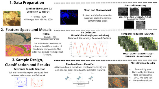
Figure 1.
Schematic representation of the methodological framework and technological tools employed in the study.
2.1. Study Area and Land Use/Land Cover Context
The Caatinga biome, an exclusive Brazilian ecosystem located in the northeastern portion of the country (Figure 2A), covers approximately 862,818 km2, representing about 10.1% of Brazil’s territory. It intersects with nine Brazilian states: Alagoas, Bahia, Ceará, Minas Gerais, Paraíba, Pernambuco, Piauí, Rio Grande do Norte, and Sergipe.
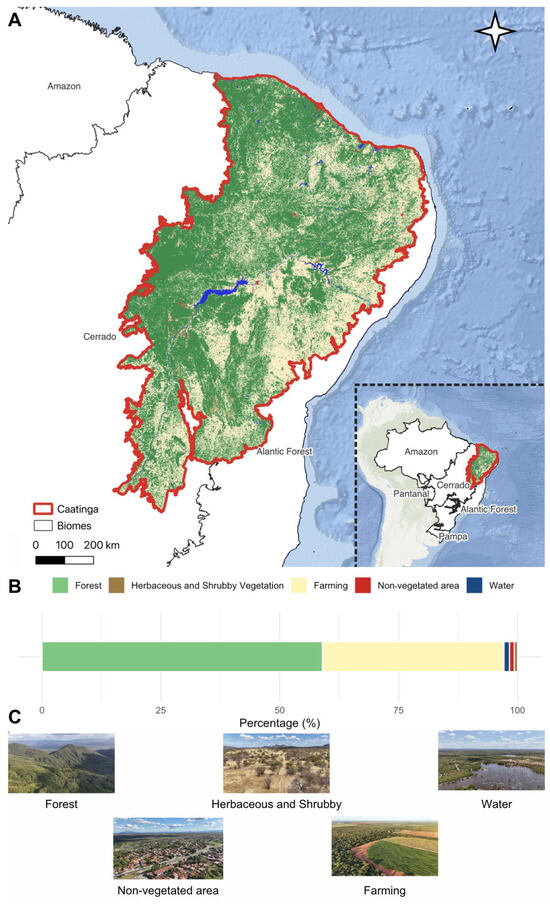
Figure 2.
Location map of the Caatinga biome. (A) Geographical context of the Caatinga and Land Use and Land Cover (LULC) map. (B) LULC chart, based on MapBiomas Collection 9, presents the dominant categories: Forest, Herbaceous and Shrubby Vegetation, Farming, Non-vegetated Areas, and Water Bodies. (C) Field images representing LULC provide visual examples of the landscape characteristics across the Caatinga biome. LULC data shown in this figure were derived from MapBiomas Collection 8, the most recent version, to provide a current overview of the study area.
The biome is characterized by its semi-arid conditions, irregular rainfall ranging from 240 to 1500 mm annually, and high insolation rates [5,31]. Droughts in this biome can persist for several months, shaping a unique vegetation dominated by xerophytic and deciduous species adapted to prolonged dry periods [32]. The dominant landscape is a mosaic of thorny shrubs, small-leaved trees, herbaceous vegetation, and cacti interspersed with rocky outcrops and intermittent rivers (Figure 2C) [32]. Despite its harsh conditions, the Caatinga hosts rich biodiversity, including numerous endemic species [32,33].
Currently, native vegetation remains the predominant land cover in the Caatinga, covering approximately 50.85 million hectares, followed by agricultural and grazing lands that extend over 32.94 million hectares (Figure 2B) [5]. From 1985 to 2019, the Caatinga lost approximately 6.57 million hectares of native vegetation, driven by agricultural and grazing expansion, with agrarian lands increasing by 284% [5].
This rapid transformation is reflected in the number of deforestation alerts, with the biome accounting for 18.4% of Brazil’s deforestation alerts in 2022 [6]. These findings emphasize the critical need for conservation and sustainable land management strategies to mitigate further degradation and preserve the fragile biome.
2.2. Data Preparation
This study employed the Google Earth Engine (GEE) platform for processing the Landsat Surface Reflectance Tier 1 time series from 1985 to 2022 (30 m spatial resolution/16 day temporal resolution) using Python 3.2 and JavaScript APIs 1.6.2. The dataset consists of images from Landsat 5 TM, Landsat 7 ETM+, and Landsat 8 OLI, harmonized using regression coefficients for the OLI sensor [34]. All images were filtered based on cloud cover, retaining only those with less than 80% cloud contamination. Cloud and shadow masks derived from the ‘pixel_qa’ band were also applied to remove atmospheric noise from the Landsat images.
A Spectral Mixture Analysis (SMA) model was applied to each image using the unmix function in GEE, based on endmembers from multiple sources, including Green Vegetation (GV), Non-Photosynthetic Vegetation (NPV), Shade, Soil [35], and Cloud [16]. A constrained model was adopted, ensuring that the sum of fractional values equaled 1 and preventing negative values.
2.3. Feature Space and Mosaic
To enhance the differentiation of landscape components, we applied the Normalized Difference Fraction Index Adjusted (NDFIa), a spectral index derived from the Spectral Mixture Analysis (SMA) model. The NDFIa is defined as follows:
where GVshade represents the green vegetation fraction corrected for shade, NPV corresponds to non-photosynthetic vegetation, and SOIL denotes the soil fraction. This index ranges from −1 to 1, where dense evergreen forests tending toward values close to 1, savanna-like formations fluctuating seasonally around 0, and bare soils and degraded areas exhibiting values near −1. The NDFIa has been successfully applied in monitoring vegetation dynamics in drylands, as demonstrated in the Deforestation Alert System for the Caatinga Biome [6], where it played a key role in detecting and analyzing deforestation events in one of South America’s most extensive tropical dry forests.
We applied a 5-year moving window to generate annual representative mosaics, including two years before and after the reference year. These time series were smoothed using a harmonic model [6,36], which reduces short-term noise while preserving seasonal patterns. The harmonic model equation is defined as follows:
where represents the smoothed NDFIa value at time t, is the time-series mean, and and are the regression coefficients for the annual and semi-annual harmonics. The term j represents the frequency components, where j = 1 corresponds to the annual cycle and j = 2 to the semi-annual cycle. The denominator 365.25 accounts for the number of days in a year, ensuring proper temporal scaling. The residual term represents unexplained variations in the time series. This model ensures a more stable representation of vegetation seasonality while minimizing artifacts caused by outliers or anomalous observations.
The final mosaics by year were composed using statistical reducers, including mean, median, mode, minimum, maximum, standard deviation, variance, and range, which provided a comprehensive representation of landscape conditions (see more details in Supplementary Materials Table S1). These statistical metrics captured both central tendencies and variability within the time series, allowing for a robust characterization of landscape changes and improving the distinction between different LULC types.
2.4. Sample Design, Classification, and Results
Annual harmonic mosaics were used as input data to classify persistent bare soils. These mosaics were generated exclusively from temporal indices, including mean, median, mode, minimum, maximum, standard deviation, variance, and range, all derived from the smoothed NDFIa time series in the Caatinga biome. This approach ensured a robust representation of LULC dynamics, reducing short-term noise while capturing long-term trends in bare soil patterns.
Reference samples were selected based on 5-year stable pixels extracted from the MapBiomas Collection 4.1 dataset [15]. The non-exposed soil samples were obtained from MapBiomas and varied annually due to the seasonal dynamics of the dataset, ensuring that classifications accounted for interannual variations in vegetation cover. In contrast, the exposed soil samples represented a unique dataset derived from field studies in areas identified by experts as persistent bare soil regions. These points were later verified using high-resolution imagery to ensure consistent exposure over time, excluding short-term or transitional cases. This fixed dataset was used due to the nature of the target class, as spectral variations in persistent bare soils are not significantly affected by annual fluctuations, unlike vegetated areas.
A Random Forest classifier (ee. Classifier. smile Random Forest) was implemented within Google Earth Engine (GEE). This classifier constructs an ensemble of decision trees, where each tree independently classifies the input data, and the final class is determined through majority voting [8]. Based on performance tests, the classifier was set to use 56 trees, 3 variables per split, and a minimum leaf population of 25, ensuring a balance between model complexity and generalization.
The classification was conducted by hydrographic basins, maintaining a consistent non-exposed soil dataset and ensuring a spatially representative classification of persistent bare soils in the Caatinga biome.
After classification, a masking process was applied to remove urban areas using the MapBiomas dataset. A frequency filter was applied to improve classification consistency, removing areas classified as exposed soil for five years or less throughout the time series. Additionally, a temporal filter with a 3-year window was implemented, where the classification of the middle year was adjusted to match the dominant class of the preceding and succeeding years. These post-processing steps ensured a more stable and reliable identification of persistent bare soils, minimizing short-term classification inconsistencies and reducing noise in the final dataset.
To conduct a preliminary accuracy assessment of the persistent bare soil classification, we randomly sampled 600 points within areas mapped as persistent bare soil in 2018. The evaluation was based on high-resolution NICFI mosaics and carried out independently by two experienced analysts. A total of 54 points were removed due to disagreement or inconclusive interpretation, resulting in 546 points with confirmed consensus. These were used to estimate the commission error of the classification. This approach ensures greater confidence in the validation data while acknowledging the limitation of not addressing omission error at this stage.
3. Results
The results of this study present the temporal and spatial dynamics of bare soils in the Caatinga biome. Of the 546 valid points used to assess commission error, 513 were confirmed as persistent bare soil by both analysts, while 33 were not. This corresponds to a commission accuracy of 93.95% and a commission error of 6.05% for the year 2018, based on high-resolution NICFI mosaics.
Figure 3 provides an overview of these patterns, illustrating areas with increased and decreased soil exposure over time. To generate the spatial representation (Figure 3A), the annual rate of soil exposure change was calculated for each hexagon, followed by an average of these values across the study period. The spatial distribution highlights regions where soil exposure has intensified, while the temporal analysis identifies specific periods of more significant change. The data are presented in different panels, showing spatial trends (Figure 3A), examples through remote sensing and field observations (Figure 3B), a time series of bare soils (Figure 3C), and aggregated data in five-year intervals (Figure 3D).
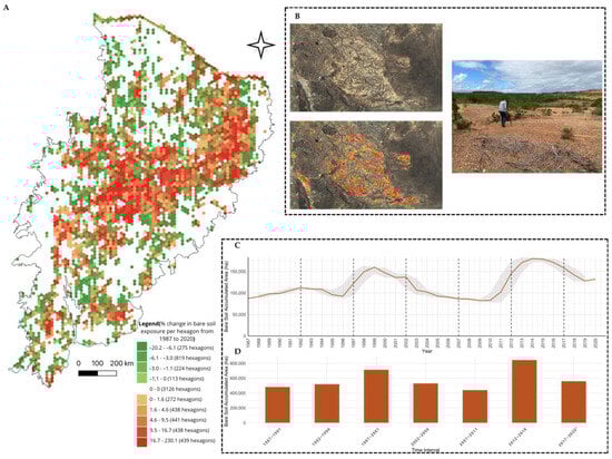
Figure 3.
Spatial and temporal patterns of persistent bare soil in the Caatinga biome. (A) Average annual percentage change in bare soil area per hexagon between 1987 and 2020. Values were calculated by averaging year-to-year percentage changes in bare soil exposure within each hexagon. Red tones indicate increasing trends, green tones indicate decreasing trends, and white areas represent stable or data-deficient regions. (B) Remote sensing and field examples. (C) Time series of bare soil area. (D) Aggregated bare soil data in five-year intervals.
Over the study period, the mapping of bare soils shows significant spatial and temporal variations. A total of 6200 hexagons were classified based on changes in soil exposure, with 2275 hexagons (36.7%) showing a reduction (green tones) and 3925 hexagons (63.3%) indicating an increase (red tones). The most affected category, representing increases between 1.46% and 9.45%, accounted for 1438 hexagons (23.2%), followed by the category with the highest growth (10.7% to 23.03%), which comprised 439 hexagons (7.1%).
This spatial distribution is presented in Figure 3A, where red tones indicate areas with increased soil exposure, while green tones represent decreased regions. Figure 3B provides visual evidence of the persistent bare soil occurrence.
The temporal dynamics of bare soils are displayed in Figure 3C,D. The time series in Figure 3C shows fluctuations in the bare soil area from 1987 to 2020, with peaks surpassing 150,000 ha during 1997–2001 and 2012–2016. The lowest recorded value was 82,000 ha, while the maximum reached 179,387 ha, with an average of 120,099 ha. The aggregated data in Figure 3D reveals that the highest cumulative soil exposure occurred in 1997–2001 and 2012–2016, exceeding 700,000 ha, while 2002–2006 and 2007–2011 exhibited lower values, staying below 400,000 ha. The most recent period (2017–2021) remains elevated.
The ranking of bare soil areas in 2020 highlights significant spatial patterns across different territorial divisions (Figure 4). Figure 4A presents the ranking by state, showing that Bahia had the largest occurrence area, totaling 65,734 ha, followed by Ceará (28,799 ha) and Rio Grande do Norte (14,273 ha). Pernambuco and Piauí also showed considerable areas of bare soil, with 10,996 ha and 6586 ha, respectively. The states with the smallest areas were Minas Gerais, Alagoas, and Sergipe.
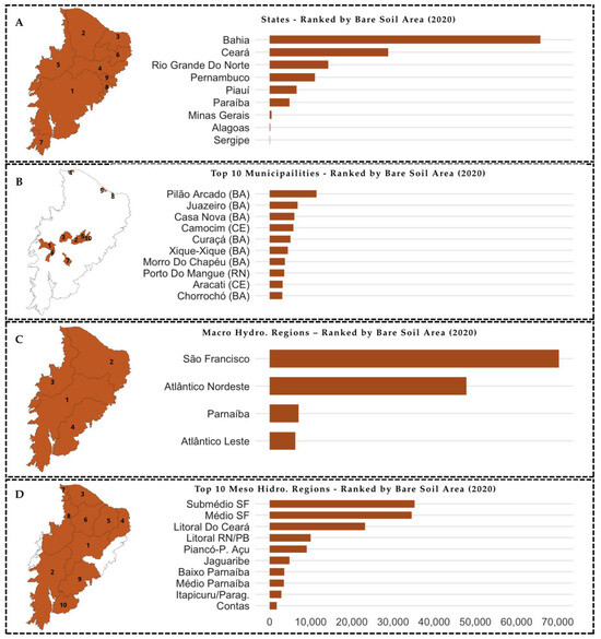
Figure 4.
Spatial distribution and ranking of bare soil occurrence in 2020 within the Caatinga biome, organized by different territorial divisions. The maps show the geographic location of the top-ranked areas, with numbers indicating their position in each ranking. (A) States: ranking of Brazilian states by bare soil area. (B) Municipalities: ranking of municipalities by bare soil area. (C) Macro Hydrographic Regions: ranking of large hydrographic regions by bare soil area (D) Meso Hydrographic Regions: ranking of smaller hydrographic regions by bare soil area.
At the municipal level (Figure 4B), the ranking indicates that Pilão Arcado (BA) recorded the highest bare soil occurrence, totaling 11,410 ha, followed by Juazeiro (BA) with 6831 ha and Casa Nova (BA) with 5981 ha. The Camocim (CE) and Curaçá (BA) municipalities also exhibited significant values, with 5770 ha and 5093 ha, respectively.
The ranking by major hydrographic basins (Figure 4C) shows that the São Francisco Basin had the largest bare soil occurrence, totaling 70,286 ha, followed by the Atlântico Nordeste Oriental Basin with 47,821 ha. The Parnaíba Basin (7058 ha) and Atlântico Leste Basin (6288 ha) also showed notable values.
At the regional watershed level (Figure 4D), the Submédio São Francisco and Médio São Francisco regions accounted for the highest bare soil occurrences, with 35,232 ha and 34,543 ha, respectively. The Litoral do Ceará region followed with 23,227 ha. Other watersheds, such as Piancó-Piranhas-Açu (9011 ha) and Jaguaribe (8421 ha), also contributed significantly to the total affected area. These rankings provide a detailed perspective on the spatial distribution of bare soil across different territorial scales, supporting further discussion on the underlying drivers of this phenomenon.
Figure 5 shows the frequency of bare soil occurrence across the study period, and Figure 5A presents a cumulative map of all annual bare soil classifications. Each pixel value represents the number of times it was identified as bare soil throughout the study period. The scale ranges from six to thirty-four occurrences. The mapped results are further illustrated with zoomed-in areas that show the temporal progression of bare soil exposure and its spatial distribution.
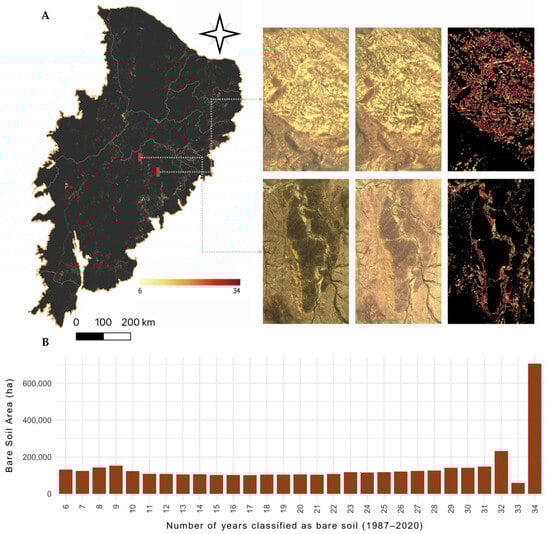
Figure 5.
Frequency of persistent bare soil occurrence in the Caatinga biome. (A) Map showing the number of years each pixel was classified as bare soil. (B) Histogram of accumulated bare soil area per frequency interval.
Figure 5B presents a histogram of accumulated bare soil area by frequency values, showing that most pixels were classified as bare soil between six and seventeen times during the study period, with values ranging from 101,314 ha to 152,345 ha. However, a sharp increase is observed in pixels classified as bare soil more than 32 times, reaching a peak of 706,019 ha for the highest frequency category (34 occurrences). This suggests that a substantial portion of the exposed soil is recurrent, emphasizing long-term degradation trends.
The analysis of land use and land cover (LULC) conversion to bare soil reveals distinct patterns over time. Figure 6 shows the percentage of each LULC class converted into bare soil each year by comparing the bare soil area with the land cover class from the previous year. The results indicate that the Mosaic of Uses (3.4) is the predominant contributor to soil exposure, consistently representing a significant portion of conversions across the entire period. Pasture (3.1) also plays a major role, maintaining a stable share over time, while Agriculture (3.2) becomes increasingly relevant, particularly after 2010.
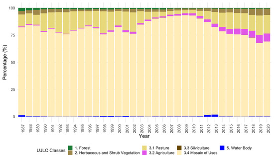
Figure 6.
Land use and land cover (LULC) classes converted to bare soil over time, based on MapBiomas Collection 4.1. Natural classes include Forest and Herbaceous and Shrub Vegetation, while Pasture, Agriculture, Silviculture, and Mosaic of Uses represent anthropic areas. Water bodies are also shown. Collection 4.1 was used to ensure independence from the bare soil data generated in this study.
When considering land use classes, anthropogenic activities were the primary drivers of soil exposure. Mosaic of Uses (3.4), Pasture (3.1), and Agriculture (3.2) accounted for the highest percentages of conversion to bare soil, reflecting the influence of human-managed landscapes. In contrast, land cover classes such as Forest (1) and Herbaceous and Shrub Vegetation (2) had minimal direct conversion to bare soil. Water Bodies (5) showed small fluctuations, likely related to hydrological changes and rainfall indexes.
A significant shift was observed after 2012 when Agriculture (3.2) and Pasture (3.1) began to increase their relative share of conversion to bare soil.
Figure 7 provides a comprehensive synthesis of persistent bare soil transitions across the study period, illustrating spatial and temporal patterns of soil exposure, including areas of expansion, reduction, and stability. Figure 7A displays a hexagonal map comparing the first and last year of the analysis, highlighting regions with significant changes. The first map (left) shows areas where bare soil expanded the most (toSoil category), represented in red tones, with the highest concentration in the central and eastern portions of the study area. The second map (center) illustrates regions where soil exposure decreased (toNoSoil category), marked in green, showing a more scattered distribution. The third map (right) presents stable bare soil areas (Soil category) in blue, indicating regions where soil exposure persisted throughout the study period.
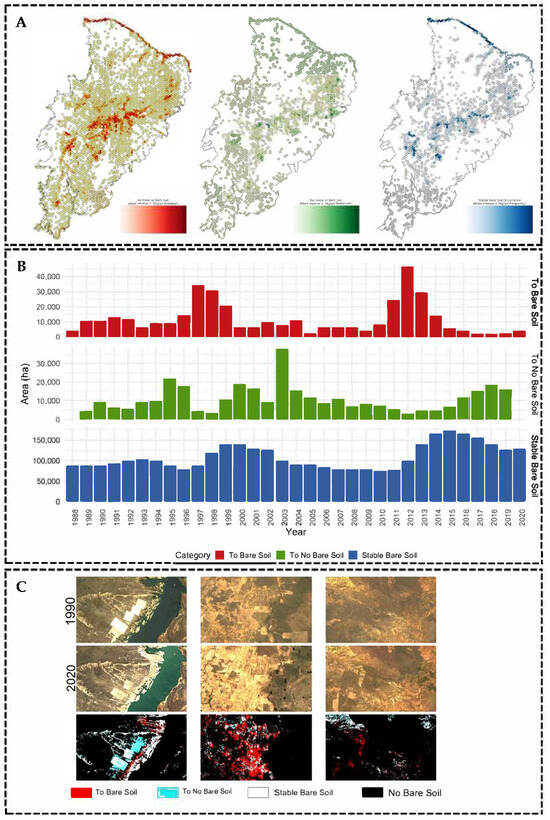
Figure 7.
Spatial and temporal transitions of persistent bare soil. (A) Hexagonal maps illustrate the spatial distribution of transitions in bare soil exposure: increase (red), decrease (green), and stability (blue). These transitions are derived from pixel-level analyses aggregated by hexagon; therefore, a single hexagon may contain pixels belonging to more than one transition. (B) Annual transitions of bare soil: conversion to bare soil (red), recovery to no bare soil (green), and stable bare soil areas (blue). (C) Examples of areas of bare soil expansion (red), recovery (cyan), persistence (white), and absence (black).
The annual transitions in bare soil dynamics are detailed in Figure 7B, which presents three bar charts. The first chart (red) represents areas transitioning to bare soil, with peaks exceeding 46,685 ha, particularly in the mid-1990s and early 2010s. The second chart (green) shows areas transitioning to no bare soil, reaching 37,962 ha in some years. The third chart (blue) represents stable bare soil areas, which remained consistently high throughout the period but increased notably after 2010, reinforcing the persistence of soil exposure in specific regions.
Figure 7C compares satellite imagery from 1990 and 2020 in selected areas to illustrate these transitions at a finer scale. The upper images show the yearly landscaping, while the lower images highlight classified transitions: areas that changed to bare soil (red), areas that recovered to no bare soil (cyan), stable bare soil (white), and no bare soils (black).
4. Discussion
This study provides the first comprehensive, long-term mapping of persistent bare soil in the Caatinga biome, contributing to a broader understanding of the spatial and temporal dynamics of land degradation in this semi-arid region. By analyzing over three decades of Landsat data, we revealed consistent and widespread patterns of soil exposure, highlighting areas under increasing environmental pressure.
In the absence of prior studies focused specifically on exposed soil in the Caatinga, our results work as a critical baseline for future comparisons. On the other hand, this novelty also presents a challenge: the lack of established benchmarks or region-specific studies makes direct quantitative comparisons difficult. Nevertheless, the patterns identified, particularly in central and eastern zones and within the São Francisco Basin, point to long-term land degradation processes.
The results indicate a widespread expansion of bare soil, particularly in the central and eastern regions, mainly in the São Francisco watershed, with more than 63% of mapped hexagons showing an increase in bare soil exposure. While certain areas exhibited signs of recovery, the persistence of bare soil remained high, with a peak exceeding 172,000 ha. The Mosaic of Uses and Pasture classes were the primary converted areas, with agriculture becoming increasingly relevant after 2010. These findings emphasize the importance of mapping bare soil as a quantifiable indicator of land degradation, providing essential insights for monitoring environmental changes, assessing the impacts of human activities, and supporting policies aimed at sustainable land management in dryland regions [1,37].
A noteworthy feature of the temporal trajectory is the marked increase in bare soil during two distinct periods: 1997–2001 and 2012–2016. These intervals coincide with extreme drought events that significantly impacted the Caatinga biome [38,39,40,41]. In particular, the 2012–2016 drought is recognized as one of the most severe —intensified by the 2015–2016 El Niño— ever recorded in Northeast Brazil [39]. The association between these drought events and the expansion of bare soil highlights their severe impacts on ecosystem balance and land productivity. Repeated and prolonged droughts accelerate soil degradation, reduce vegetation cover, and intensify erosion, compromising agricultural sustainability and water availability [7].
Another key finding of this study is that the São Francisco Basin exhibited the highest occurrence and most significant increase in bare soil area. This basin is one of the driest regions of the Caatinga biome, characterized by low annual rainfall and high solar radiation, making it naturally vulnerable to land degradation processes [42]. Additionally, the São Francisco Basin was the first officially recognized arid region in Brazil; climate projections also indicate an increase in arid conditions and temperature, further exacerbating water scarcity and land degradation risks [40,43]. Given its ecological fragility and social vulnerability, with a high concentration of low-income populations, this territory requires greater attention in public policies to mitigate land degradation [42,44,45,46,47].
Our research revealed a significant extent of bare soil persistence over 32–34 years, indicating long-term land exposure. While some of these areas correspond to dunes (Camocim-CE, Aracati-CE, Porto do Mangue-RN) and rock outcrops (e.g., Morro do Chapéu-BA), which are natural landscape features, their movement and expansion may also indicate degradation processes [48]. A substantial portion is linked to abandoned agricultural and livestock areas, suggesting a decline in land productivity. Additionally, new hotspots of bare soil exposure were identified, particularly in Bahia (inside and near the desertification hotspots), where areas mapped for less than 17 years have also been abandoned, mainly following the decline of pasture lands due to soil degradation and the severity and recurrence of droughts.
Although the results of this study are crucial for characterizing the expansion of land degradation in the Caatinga biome—having even contributed to the most recent MapBiomas collections—we adopted a more restrictive approach for the maps and analyses presented here.
Moving forward, we are working on methodological improvements, including developing a validation dataset specifically aimed at assessing omission errors, to complement the commission accuracy metrics already presented in the current version of the study. This is particularly challenging in the case of rare classes such as persistent bare soil, where omission errors require larger sampling efforts to be accurately detected. As highlighted in the literature, classes with low spatial frequency are often underrepresented in validation datasets, making omission assessment more difficult and resource-intensive [49].
In summary, the results of this study provide a crucial foundation for understanding land degradation in the Caatinga biome. By identifying spatial patterns, temporal trends, and underlying drivers of bare soil exposure, this work lays the groundwork for more targeted interventions, long-term monitoring, and resilience-building strategies in Brazil’s most vulnerable dryland regions.
5. Conclusions
This study demonstrated an expansion of persistent bare soil in the Caatinga biome, reinforcing its role as an indicator of land degradation in drylands. The findings revealed key areas of concern, particularly in the São Francisco Basin, where long-term soil exposure and recent land abandonment highlight the need for land management efforts. By addressing the key research questions, this study identified where and how these areas are expanding, the land use classes most affected, and the relation between prolonged droughts and soil exposure, providing a comprehensive assessment of degradation patterns.
While this research offers important insights, future studies should refine validation methods and temporal resolution to improve monitoring efficiency. Expanding the analysis to include semi-annual mapping and improved classification techniques will enhance the understanding of land degradation trends, supporting more effective conservation and land management policies in the region.
Supplementary Materials
The following supporting information can be downloaded at: https://www.mdpi.com/article/10.3390/earth6030096/s1. Table S1, List of NDFIa-adjusted mosaics used in the study, available on Google Earth Engine as ee.Image() objects. Each image corresponds to a specific year from 1987 to 2001 and is stored under the path projects/mapbiomas-arida/doctorate/mosaics_ndfia_adjusted/ followed by the respective year.
Author Contributions
Conceptualization, D.P.C., S.M.H., A.T.C.L., C.A.D.L., R.N.V., W.J.S.F.R., S.G.D., D.T.M.S., and N.A.S.; methodology, D.P.C., S.M.H., A.T.C.L., C.A.D.L., R.N.V., and S.G.D.; software execution, D.P.C., R.N.V., and N.A.S.; writing—original draft preparation, D.P.C., A.T.C.L., C.A.D.L., W.J.S.F.R., and R.N.V.; writing—review and editing, S.M.H., A.T.C.L., C.A.D.L., and W.J.S.F.R.; supervision, S.M.H., W.J.S.F.R., R.N.V., A.T.C.L., and C.A.D.L.; funding acquisition, D.P.C., W.J.S.F.R., C.A.D.L., and R.N.V. All authors have read and agreed to the published version of the manuscript.
Funding
D.P.C. was financially supported by the Bahia State Research Foundation (FAPESB) under grant #BOL 0457/2019 and by CAPES/CAPES/PRINT through grant no. 41/2017. W.J.S.F.R. was supported by a CNPQ research fellowship under Process #314954/2021-0 and the Prospecta 4.0—CNPQ research grant under Process #407907/2022-0. D.P.C., R.N.V., and W.J.S.F.R. were supported by the INCT IN-TREE for Technology in Interdisciplinary and Transdisciplinary Studies in Ecology and Evolution n° 465767/2014-1. D.P.C., R.N.V., S.G.D., and W.J.S.F.R. were supported by WRI subgrant to WRI Brazil no. 73054 related to the Land and Carbon Lab platform. Additional funding was provided by Research Support Foundation of the State of Bahia FAPESB under the program Bioresources, Water Resources, and Environmental Sustainability in Bahia, through the Postgraduate Program in Modeling in Earth and Environmental Sciences, Call for Proposals 38/2022, Technical Cooperation Agreement Nº 294/2023 and Grant Agreement Nº PPF0003/2023.
Data Availability Statement
No new data were created or analyzed in this study. Data sharing is not applicable to this article.
Acknowledgments
We extend our gratitude to the anonymous reviewers for their valuable comments and suggestions, which greatly contributed to enhancing the quality and presentation of this manuscript. We gratefully acknowledge the support provided by FAPESB, CAPES, CIENAM, and PPGM for this project.
Conflicts of Interest
The authors declare no conflicts of interest.
References
- Costa, D.P.; Herrmann, S.M.; Vasconcelos, R.N.; Duverger, S.G.; Franca Rocha, W.J.S.; Cambuí, E.C.B.; Lobão, J.S.B.; Santos, E.M.R.; Ferreira-Ferreira, J.; Oliveira, M.; et al. Bibliometric Analysis of Land Degradation Studies in Drylands Using Remote Sensing Data: A 40-Year Review. Land 2023, 12, 1721. [Google Scholar] [CrossRef]
- Mirzabaev, A.; Stringer, L.C.; Benjaminsen, T.A.; Gonzalez, P.; Harris, R.; Jafari, M.; Stevens, N.; Tirado, C.M.; Zakieldeen, S. 2022: Cross-Chapter Paper 3: Deserts, Semiarid Areas and Desertification. In Climate Change 2022: Impacts, Adaptation and Vulnerability. Contribution of Working Group II to the Sixth Assessment Report of the Intergovernmental Panel on Climate Change; Pörtner, H.-O., Roberts, D.C., Tignor, M., Poloczanska, E.S., Mintenbeck, K., Alegría, A., Craig, M., Langsdorf, S., Löschke, S., Möller, V., et al., Eds.; Cambridge University Press: Cambridge, UK, 2019; pp. 2195–2231. [Google Scholar] [CrossRef]
- Smith, W.K.; Dannenberg, M.P.; Yan, D.; Herrmann, S.; Barnes, M.L.; Barron-Gafford, G.A.; Biederman, J.A.; Ferrenberg, S.; Fox, A.M.; Hudson, A.; et al. Remote Sensing of Dryland Ecosystem Structure and Function: Progress, Challenges, and Opportunities. Remote Sens. Environ. 2019, 233, 111401. [Google Scholar] [CrossRef]
- Herrmann, S.M.; Hutchinson, C.F. The Scientific Basis: Links between Land Degradation, Drought and Desertification. In Governing Global Desertification; Routledge: Oxford, UK, 2016; pp. 31–46. [Google Scholar]
- Rocha, F.; Rocha, W.J.S.F.; Vasconcelos, R.N.; Costa, D.P.; Duverger, S.G.; Lobão, J.S.B.; Souza, D.T.M.; Herrmann, S.M.; Santos, N.A.; Franca Rocha, R.O.; et al. Towards Uncovering Three Decades of LULC in the Brazilian Drylands: Caatinga Biome Dynamics (1985–2019). Land 2024, 13, 1250. [Google Scholar] [CrossRef]
- Costa, D.P.; Lentini, C.A.D.; Cunha Lima, A.T.; Duverger, S.G.; Vasconcelos, R.N.; Herrmann, S.M.; Ferreira-Ferreira, J.; Oliveira, M.; da Silva Barbosa, L.; Cordeiro, C.L.; et al. All Deforestation Matters: Deforestation Alert System for the Caatinga Biome in South America’s Tropical Dry Forest. Sustainability 2024, 16, 9006. [Google Scholar] [CrossRef]
- Marengo, J.A.; Galdos, M.V.; Challinor, A.; Cunha, A.P.; Marin, F.R.; Vianna, M.d.S.; Alvala, R.C.S.; Alves, L.M.; Moraes, O.L.; Bender, F. Drought in Northeast Brazil: A Review of Agricultural and Policy Adaptation Options for Food Security. Clim. Resil. Sustain. 2022, 1, e17. [Google Scholar] [CrossRef]
- Belgiu, M.; Drăgu, L. Random Forest in Remote Sensing: A Review of Applications and Future Directions. ISPRS J. Photogramm. Remote Sens. 2016, 114, 24–31. [Google Scholar] [CrossRef]
- Herrmann, S.M.; Brandt, M.; Rasmussen, K.; Fensholt, R. Accelerating Land Cover Change in West Africa over Four Decades as Population Pressure Increased. Commun. Earth Environ. 2020, 1, 53. [Google Scholar] [CrossRef]
- Robinove, C.J.; Chavez, P.S.; Gehring, D.; Holmgren, R. Arid Land Monitoring Using Landsat Albedo Difference Images. Remote Sens. Environ. 1981, 11, 133–156. [Google Scholar] [CrossRef]
- Graetz, R.D. Satellite Remote Sensing of Australian Rangelands. Remote Sens. Environ. 1987, 23, 313–331. [Google Scholar] [CrossRef]
- Kumar, L.; Mutanga, O. Google Earth Engine Applications since Inception: Usage, Trends, and Potential. Remote Sens. 2018, 10, 1509. [Google Scholar] [CrossRef]
- Gorelick, N.; Hancher, M.; Dixon, M.; Ilyushchenko, S.; Thau, D.; Moore, R. Google Earth Engine: Planetary-Scale Geospatial Analysis for Everyone. Remote Sens. Environ. 2017, 202, 18–27. [Google Scholar] [CrossRef]
- Sidhu, N.; Pebesma, E.; Câmara, G. Using Google Earth Engine to Detect Land Cover Change: Singapore as a Use Case Using Google Earth Engine to Detect Land Cover Change: Singapore as a Use. Eur. J. Remote Sens. 2018, 51, 486–500. [Google Scholar] [CrossRef]
- Souza, C.M.; Shimbo, J.Z.; Rosa, M.R.; Parente, L.L.; Alencar, A.A.; Rudorff, B.F.T.; Hasenack, H.; Matsumoto, M.; Ferreira, L.G.; Souza-Filho, P.W.M.; et al. Reconstructing Three Decades of Land Use and Land Cover Changes in Brazilian Biomes with Landsat Archive and Earth Engine. Remote Sens. 2020, 12, 2735. [Google Scholar] [CrossRef]
- Bullock, E.L.; Woodcock, C.E.; Olofsson, P. Monitoring Tropical Forest Degradation Using Spectral Unmixing and Landsat Time Series Analysis. Remote Sens. Environ. 2018, 238, 110968. [Google Scholar] [CrossRef]
- Souza, C.; Barreto, P. An Alternative Approach for Detecting and Monitoring Selectively Logged Forests in the Amazon. Int. J. Remote Sens. 2000, 21, 173–179. [Google Scholar] [CrossRef]
- Hansen, M.C.; Krylov, A.; Tyukavina, A.; Potapov, P.V.; Turubanova, S.; Zutta, B.; Ifo, S.; Margono, B.; Stolle, F.; Moore, R. Humid Tropical Forest Disturbance Alerts Using Landsat Data. Environ. Res. Lett. 2016, 11, 034008. [Google Scholar] [CrossRef]
- Sofan, P.; Vetrita, Y.; Yulianto, F.; Khomarudin, M.R. Multi-Temporal Remote Sensing Data and Spectral Indices Analysis for Detection Tropical Rainforest Degradation: Case Study in Kapuas Hulu and Sintang Districts, West Kalimantan, Indonesia. Nat. Hazards 2016, 80, 1279–1301. [Google Scholar] [CrossRef]
- Marengo, J.A.; Bernasconi, M. Regional Differences in Aridity/Drought Conditions over Northeast Brazil: Present State and Future Projections. Clim. Change 2015, 129, 103–115. [Google Scholar] [CrossRef]
- Lomax, G.A.; Powell, T.W.R.; Lenton, T.M.; Cunliffe, A.M. The Relative Productivity Index: Mapping Human Impacts on Rangeland Vegetation Productivity with Quantile Regression Forests. Ecol. Indic. 2025, 171, 113208. [Google Scholar] [CrossRef]
- Xie, H.; Zhang, Y.; Wu, Z.; Lv, T. A Bibliometric Analysis on Land Degradation: Current Status, Development, and Future Directions. Land 2020, 9, 28. [Google Scholar] [CrossRef]
- Wiethase, J.H.; Critchlow, R.; Foley, C.; Foley, L.; Kinsey, E.J.; Bergman, B.G.; Osujaki, B.; Mbwambo, Z.; Kirway, P.B.; Redeker, K.R.; et al. Pathways of Degradation in Rangelands in Northern Tanzania Show Their Loss of Resistance, but Potential for Recovery. Sci. Rep. 2023, 13, 2417. [Google Scholar] [CrossRef] [PubMed]
- Lehmann, J.; Kleber, M. The Contentious Nature of Soil Organic Matter. Nature 2015, 528, 60–68. [Google Scholar] [CrossRef] [PubMed]
- Stringer, L.C.; Reed, M.S. Land Degradation Assessment in Southern Africa: Integrating Local and Scientific Knowledge Bases. Land. Degrad. Dev. 2007, 18, 99–116. [Google Scholar] [CrossRef]
- Small, C.; Milesi, C. Multi-Scale Standardized Spectral Mixture Models. Remote Sens. Environ. 2013, 136, 442–454. [Google Scholar] [CrossRef]
- Souza, C.M.; Siqueira, J.V.; Sales, M.H.; Fonseca, A.V.; Ribeiro, J.G.; Numata, I.; Cochrane, M.A.; Barber, C.P.; Roberts, D.A.; Barlow, J. Ten-Year Landsat Classification of Deforestation and Forest Degradation in the Brazilian Amazon. Remote Sens. 2013, 5, 5493–5513. [Google Scholar] [CrossRef]
- Yang, J.; Weisberg, P.J.; Bristow, N.A. Landsat Remote Sensing Approaches for Monitoring Long-Term Tree Cover Dynamics in Semi-Arid Woodlands: Comparison of Vegetation Indices and Spectral Mixture Analysis. Remote Sens. Environ. 2012, 119, 62–71. [Google Scholar] [CrossRef]
- Antongiovanni, M.; Venticinque, E.M.; Fonseca, C.R. Fragmentation Patterns of the Caatinga Drylands. Landsc. Ecol. 2018, 33, 1353–1367. [Google Scholar] [CrossRef]
- Alencar, A.A.C.; Arruda, V.L.S.; da Silva, W.V.; Conciani, D.E.; Costa, D.P.; Crusco, N.; Duverger, S.G.; Ferreira, N.C.; Franca-Rocha, W.; Hasenack, H.; et al. Long-Term Landsat-Based Monthly Burned Area Dataset for the Brazilian Biomes Using Deep Learning. Remote Sens. 2022, 14, 2510. [Google Scholar] [CrossRef]
- Braga, A.; Laurini, M. Spatial Heterogeneity in Climate Change Effects across Brazilian Biomes. Sci. Rep. 2024, 14, 16414. [Google Scholar] [CrossRef]
- Leal, I.R.; Da Silva, J.M.C.; Tabarelli, M.; Lacher, T.E., Jr. Changing the Course of Biodiversity Conservation in the Caatinga of Northeastern Brazil. Wiley: Hoboken, NJ, USA, 2005. [Google Scholar]
- Araujo, H.F.P.; Canassa, N.F.; Machado, C.C.C.; Tabarelli, M. Human Disturbance Is the Major Driver of Vegetation Changes in the Caatinga Dry Forest Region. Sci. Rep. 2023, 13, 18440. [Google Scholar] [CrossRef]
- Roy, D.P.; Kovalskyy, V.; Zhang, H.K.; Vermote, E.F.; Yan, L.; Kumar, S.S.; Egorov, A. Characterization of Landsat-7 to Landsat-8 Reflective Wavelength and Normalized Difference Vegetation Index Continuity. Remote Sens. Environ. 2016, 185, 57–70. [Google Scholar] [CrossRef] [PubMed]
- Souza, C.M.; Roberts, D.A.; Cochrane, M.A. Combining Spectral and Spatial Information to Map Canopy Damage from Selective Logging and Forest Fires. Remote Sens. Environ. 2005, 98, 329–343. [Google Scholar] [CrossRef]
- Lentini, C.A.D.; Campos, E.J.D.; Podestá, G.G. The Annual Cycle of Satellite Derived Sea Surface Temperature on the Western South Atlantic Shelf. Rev. Bras. Oceanogr. 2000, 48, 93–105. [Google Scholar] [CrossRef]
- Demattê, J.A.M.; Safanelli, J.L.; Poppiel, R.R.; Rizzo, R.; Silvero, N.E.Q.; Mendes, W.d.S.; Bonfatti, B.R.; Dotto, A.C.; Salazar, D.F.U.; Mello, F.A. de O.; et al. Bare Earth’s Surface Spectra as a Proxy for Soil Resource Monitoring. Sci. Rep. 2020, 10, 4461. [Google Scholar] [CrossRef]
- da Silva Júnior, I.B.; da Silva Araújo, L.; Stosic, T.; Menezes, R.S.C.; da Silva, A.S.A. Space-Time Variability of Drought Characteristics in Pernambuco, Brazil. Water 2024, 16, 1490. [Google Scholar] [CrossRef]
- Cunha, A.P.M.A.; Zeri, M.; Leal, K.D.; Costa, L.; Cuartas, L.A.; Marengo, J.A.; Tomasella, J.; Vieira, R.M.; Barbosa, A.A.; Cunningham, C.; et al. Extreme Drought Events over Brazil from 2011 to 2019. Atmosphere 2019, 10, 642. [Google Scholar] [CrossRef]
- Marengo, J.A.; Cunha, A.P.M.A.; Nobre, C.A.; Ribeiro Neto, G.G.; Magalhaes, A.R.; Torres, R.R.; Sampaio, G.; Alexandre, F.; Alves, L.M.; Cuartas, L.A.; et al. Assessing Drought in the Drylands of Northeast Brazil under Regional Warming Exceeding 4 °C. Nat. Hazards 2020, 103, 2589–2611. [Google Scholar] [CrossRef]
- Marengo, J.A.; Alves, L.M.; Alvala, R.C.S.; Cunha, A.P.; Brito, S.; Moraes, O.L.L. Climatic Characteristics of the 2010-2016 Drought in the Semiarid Northeast Brazil Region. An Acad Bras Cienc 2018, 90, 1973–1985. [Google Scholar] [CrossRef]
- de Barros de Sousa, L.; de Assunção Montenegro, A.A.; da Silva, M.V.; Almeida, T.A.B.; de Carvalho, A.A.; da Silva, T.G.F.; de Lima, J.L.M.P. Spatiotemporal Analysis of Rainfall and Droughts in a Semiarid Basin of Brazil: Land Use and Land Cover Dynamics. Remote Sens. 2023, 15, 2550. [Google Scholar] [CrossRef]
- Tomasella, J.; de A. Cunha, A.P.; Marengo, J.A. Nota Técnica: Elaboração dos Mapas de índice de Aridez e Precipitação Total Acumulada para o Brasil. Available online: https://www.gov.br/cemaden/pt-br/assuntos/noticias-cemaden/estudo-do-cemaden-e-do-inpe-identifica-pela-primeira-vez-a-ocorrencia-de-uma-regiao-arida-no-pais/nota-tecnica_aridas.pdf (accessed on 29 November 2023).
- Sun, T.; Ferreira, V.G.; He, X.; Andam-Akorful, S.A. Water Availability of São Francisco River Basin Based on a Space-Borne Geodetic Sensor. Water 2016, 8, 213. [Google Scholar] [CrossRef]
- Andrade, C.; de Souza, I.; da Silva, L. The Future Sustainability of the São Francisco River Basin in Brazil: A Case Study. Sustainability 2024, 16, 5521. [Google Scholar] [CrossRef]
- Paredes-Trejo, F.; Barbosa, H.A.; Daldegan, G.A.; Teich, I.; García, C.L.; Kumar, T.V.L.; Buriti, C.d.O. Impact of Drought on Land Productivity and Degradation in the Brazilian Semiarid Region. Land 2023, 12, 954. [Google Scholar] [CrossRef]
- Jardim, A.M.d.R.F.; Araújo Júnior, G.D.N.; da Silva, M.V.; Dos Santos, A.; da Silva, J.L.B.; Pandorfi, H.; de Oliveira-Júnior, J.F.; Teixeira, A.H.d.C.; Teodoro, P.E.; de Lima, J.L.M.P.; et al. Using Remote Sensing to Quantify the Joint Effects of Climate and Land Use/Land Cover Changes on the Caatinga Biome of Northeast Brazilian. Remote Sens. 2022, 14, 1911. [Google Scholar] [CrossRef]
- Abdelfattah, M.A. Land Degradation Indicators and Management Options in the Desert Environment of Abu Dhabi, United Arab Emirates. Soil. Horizons 2009, 50, 3–10. [Google Scholar] [CrossRef]
- Foody, G.M. Status of Land Cover Classification Accuracy Assessment. Remote Sens. Environ. 2002, 80, 185–201. [Google Scholar] [CrossRef]
Disclaimer/Publisher’s Note: The statements, opinions and data contained in all publications are solely those of the individual author(s) and contributor(s) and not of MDPI and/or the editor(s). MDPI and/or the editor(s) disclaim responsibility for any injury to people or property resulting from any ideas, methods, instructions or products referred to in the content. |
© 2025 by the authors. Licensee MDPI, Basel, Switzerland. This article is an open access article distributed under the terms and conditions of the Creative Commons Attribution (CC BY) license (https://creativecommons.org/licenses/by/4.0/).