
Uncertainties and Perspectives on Forest Height Estimates by Sentinel-1 Interferometry


Abstract
:1. Introduction
2. Materials and Methods
2.1. Sentinel 1 Data
2.2. Interferometric Phase Modelling
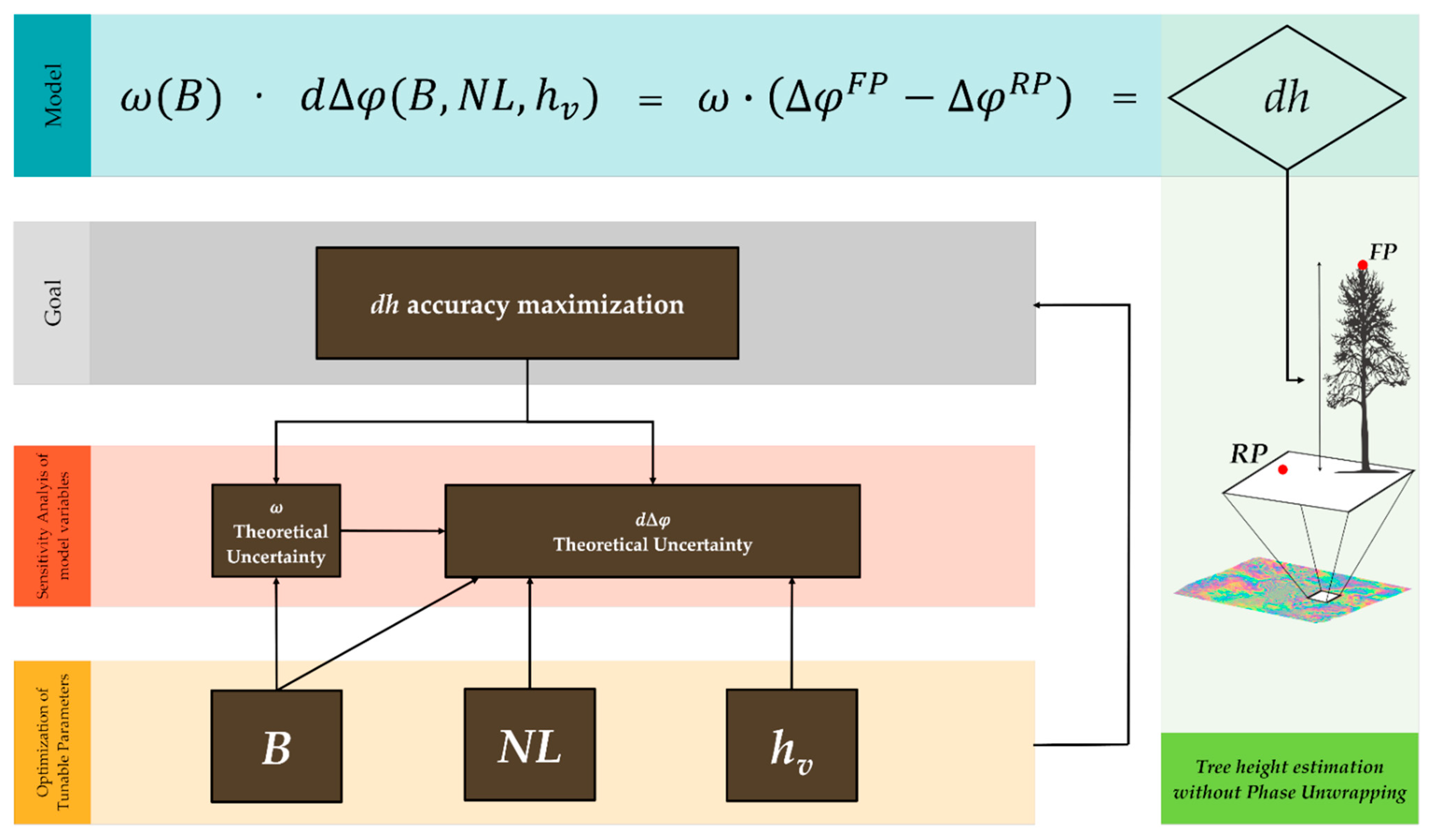
2.3. Modelling dh Uncertainty
2.3.1. Theoretical Uncertainty of ω
2.3.2. Theoretical Uncertainty of
2.4. Minimizing through Simulated Scenarios
3. Results and Discussion
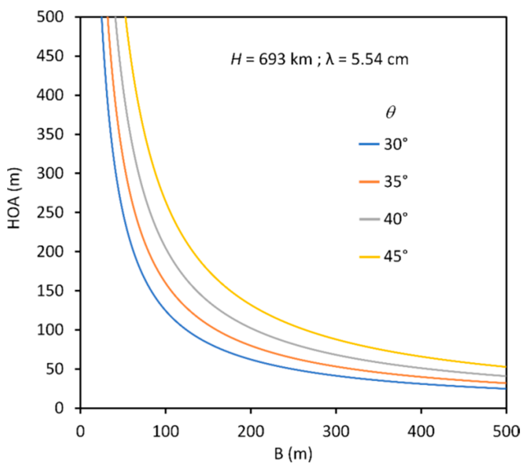
3.1. Theoretical Uncertainty of
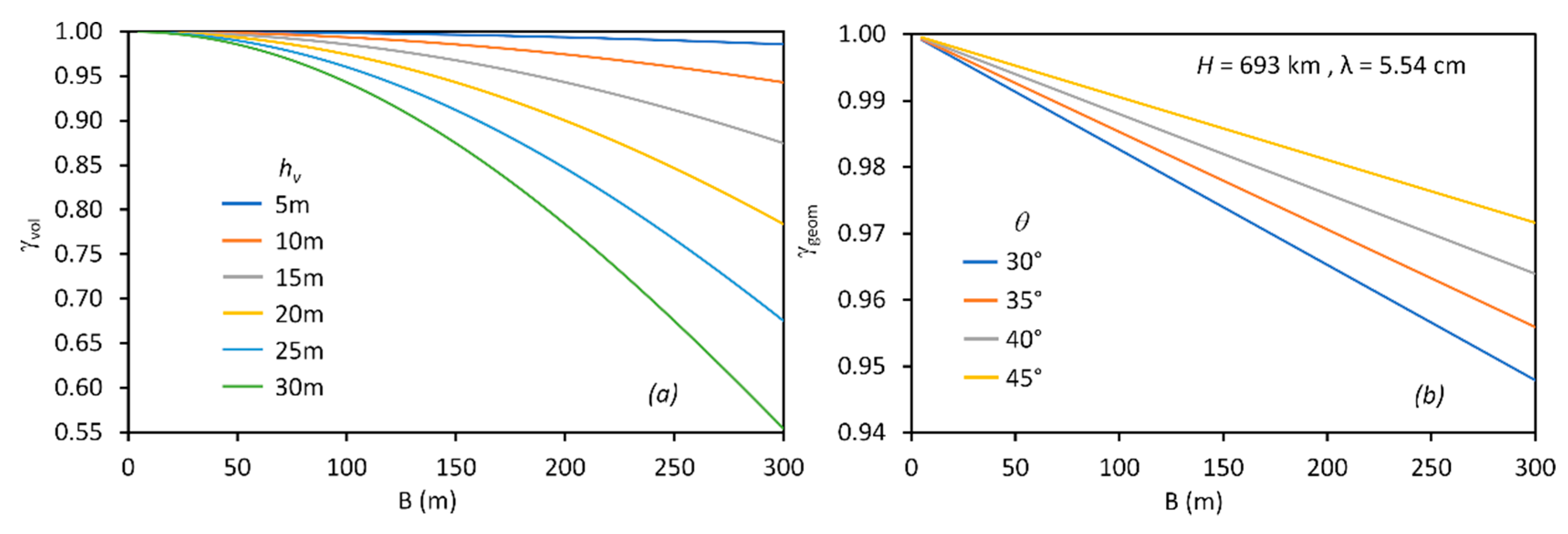
3.2. Theoretical Uncertainty of
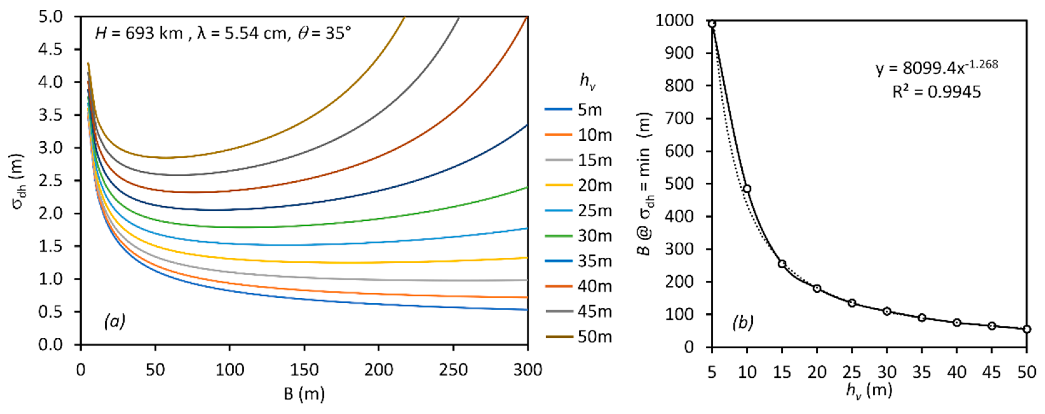
3.3. Minimizing through Simulated Scenarios
4. Conclusions
Author Contributions
Funding
Institutional Review Board Statement
Informed Consent Statement
Data Availability Statement
Conflicts of Interest
References
- Segura, M.; Kanninen, M. Allometric Models for Tree Volume and Total Aboveground Biomass in a Tropical Humid Forest in Costa Rica. Biotrop. J. Biol. Conserv. 2005, 37, 2–8. [Google Scholar]
- Laurin, G.V.; Ding, J.; Disney, M.; Bartholomeus, H.; Herold, M.; Papale, D.; Valentini, R. Tree Height in Tropical Forest as Measured by Different Ground, Proximal, and Remote Sensing Instruments, and Impacts on above Ground Biomass Estimates. Int. J. Appl. Earth Obs. Geoinf. 2019, 82, 101899. [Google Scholar] [CrossRef]
- Hao, Z.; Zhang, J.; Song, B.; Ye, J.; Li, B. Vertical Structure and Spatial Associations of Dominant Tree Species in an Old-Growth Temperate Forest. For. Ecol. Manag. 2007, 252, 1–11. [Google Scholar] [CrossRef]
- Song, B.; Chen, J.; Desander, P.V.; Reed, D.D.; Bradshaw, G.A.; Franklin, J.F. Modeling Canopy Structure and Heterogeneity across Scales: From Crowns to Canopy. For. Ecol. Manag. 1997, 96, 217–229. [Google Scholar] [CrossRef]
- Spies, T.A. Forest Structure: A Key to the Ecosystem. Northwest Sci. 1998, 72, 34–36. [Google Scholar]
- Lund, H.G. When Is a Forest Not a Forest? J. For. 2002, 100, 21–28. [Google Scholar]
- Sillett, S.C.; Van Pelt, R.; Koch, G.W.; Ambrose, A.R.; Carroll, A.L.; Antoine, M.E.; Mifsud, B.M. Increasing Wood Production through Old Age in Tall Trees. For. Ecol. Manag. 2010, 259, 976–994. [Google Scholar] [CrossRef]
- Hanewinkel, M.; Hummel, S.; Albrecht, A. Assessing Natural Hazards in Forestry for Risk Management: A Review. Eur. J. For. Res. 2011, 130, 329–351. [Google Scholar] [CrossRef]
- Martins, A.C.; Willig, M.R.; Presley, S.J.; Marinho-Filho, J. Effects of Forest Height and Vertical Complexity on Abundance and Biodiversity of Bats in Amazonia. For. Ecol. Manag. 2017, 391, 427–435. [Google Scholar] [CrossRef]
- Bohn, F.J.; Huth, A. The Importance of Forest Structure to Biodiversity–Productivity Relationships. R. Soc. Open Sci. 2017, 4, 160521. [Google Scholar] [CrossRef] [Green Version]
- Bragg, D.C. Accurately Measuring the Height of (Real) Forest Trees. J. For. 2014, 112, 51–54. [Google Scholar] [CrossRef] [Green Version]
- Larsen, D.R.; Hann, D.W.; Stearns-Smith, S.C. Accuracy and Precision of the Tangent Method of Measuring Tree Height. West. J. Appl. For. 1987, 2, 26–28. [Google Scholar] [CrossRef]
- De Petris, S.; Berretti, R.; Sarvia, F.; Borgogno Mondino, E. When a Definition Makes the Difference: Operative Issues about Tree Height Measures from RPAS-Derived CHMs. iFor.-Biogeosci. For. 2020, 13, 404. [Google Scholar] [CrossRef]
- Hüttich, C.; Eberle, J.; Shvidenko, A.; Schepaschenko, D. Supporting a Forest Observation System for Siberia: Earth Observation for Monitoring, Assessing and Providing Forest Resource Information. Ecosystems 2014. Available online: https://earthzine.org/supporting-a-forest-observation-system-for-siberia-earth-observation-for-monitoring-assessing-and-providing-forest-resource-information/ (accessed on 27 February 2022).
- Goldstein, R.M.; Zebker, H.A.; Werner, C.L. Satellite Radar Interferometry: Two-Dimensional Phase Unwrapping. Radio Sci. 1988, 23, 713–720. [Google Scholar] [CrossRef] [Green Version]
- Chen, C.W.; Zebker, H.A. Phase Unwrapping for Large SAR Interferograms: Statistical Segmentation and Generalized Network Models. IEEE Trans. Geosci. Remote Sens. 2002, 40, 1709–1719. [Google Scholar] [CrossRef] [Green Version]
- Braun, A. Retrieval of Digital Elevation Models from Sentinel-1 Radar Data–Open Applications, Techniques, and Limitations. Open Geosci. 2021, 13, 532–569. [Google Scholar] [CrossRef]
- Hagberg, J.O.; Ulander, L.M.; Askne, J. Repeat-Pass SAR Interferometry over Forested Terrain. IEEE Trans. Geosci. Remote Sens. 1995, 33, 331–340. [Google Scholar] [CrossRef]
- Santoro, M.; Askne, J.; Dammert, P.B. Tree Height Influence on ERS Interferometric Phase in Boreal Forest. IEEE Trans. Geosci. Remote Sens. 2005, 43, 207–217. [Google Scholar] [CrossRef]
- Romero-Puig, N.; Lopez-Sanchez, J.M. A Review of Crop Height Retrieval Using InSAR Strategies: Techniques and Challenges. IEEE J. Sel. Top. Appl. Earth Obs. Remote Sens. 2021, 14, 7911–7930. [Google Scholar] [CrossRef]
- De Petris, S.; Sarvia, F.; Gullino, M.; Tarantino, E.; Borgogno-Mondino, E. Sentinel-1 Polarimetry to Map Apple Orchard Damage after a Storm. Remote Sens. 2021, 13, 1030. [Google Scholar] [CrossRef]
- Sarvia, F.; Xausa, E.; De Petris, S.D.; Cantamessa, G.; Borgogno-Mondino, E. A Possible Role of Copernicus Sentinel-2 Data to Support Common Agricultural Policy Controls in Agriculture. Agronomy 2021, 10, 110. [Google Scholar] [CrossRef]
- De Petris, S.; Sarvia, F.; Borgogno-Mondino, E. Multi-Temporal Mapping of Flood Damage to Crops Using Sentinel-1 Imagery: A Case Study of the Sesia River (October 2020). Remote Sens. Lett. 2021, 12, 459–469. [Google Scholar] [CrossRef]
- Vollrath, A.; Mullissa, A.; Reiche, J. Angular-Based Radiometric Slope Correction for Sentinel-1 on Google Earth Engine. Remote Sens. 2020, 12, 1867. [Google Scholar] [CrossRef]
- Reiche, J.; Lucas, R.; Mitchell, A.L.; Verbesselt, J.; Hoekman, D.H.; Haarpaintner, J.; Kellndorfer, J.M.; Rosenqvist, A.; Lehmann, E.A.; Woodcock, C.E. Combining Satellite Data for Better Tropical Forest Monitoring. Nat. Clim. Chang. 2016, 6, 120–122. [Google Scholar] [CrossRef]
- Veci, L. SENTINEL-1 Toolbox SAR Basics Tutorial; ARRAY Systems Computing, Inc.; European Space Agency: Paris, France, 2015. [Google Scholar]
- Garestier, F.; Dubois-Fernandez, P.C.; Papathanassiou, K.P. Pine Forest Height Inversion Using Single-Pass X-Band PolInSAR Data. IEEE Trans. Geosci. Remote Sens. 2007, 46, 59–68. [Google Scholar] [CrossRef]
- Managhebi, T.; Maghsoudi, Y.; Zoej, M.J.V. A Volume Optimization Method to Improve the Three-Stage Inversion Algorithm for Forest Height Estimation Using PolInSAR Data. IEEE Geosci. Remote Sens. Lett. 2018, 15, 1214–1218. [Google Scholar] [CrossRef]
- Cloude, S.R.; Chen, H.; Goodenough, D.G. Forest Height Estimation and Validation Using Tandem-X Polinsar. In Proceedings of the 2013 IEEE International Geoscience and Remote Sensing Symposium-IGARSS, Melbourne, VIC, Australia, 21–26 July 2013; pp. 1889–1892. [Google Scholar]
- Soja, M.J.; Persson, H.; Ulander, L.M. Estimation of Forest Height and Canopy Density from a Single InSAR Correlation Coefficient. IEEE Geosci. Remote Sens. Lett. 2014, 12, 646–650. [Google Scholar] [CrossRef] [Green Version]
- Askne, J.; Santoro, M. Multitemporal Repeat Pass SAR Interferometry of Boreal Forests. IEEE Trans. Geosci. Remote Sens. 2005, 43, 1219–1228. [Google Scholar] [CrossRef]
- Askne, J.I.; Dammert, P.B.; Ulander, L.M.; Smith, G. C-Band Repeat-Pass Interferometric SAR Observations of the Forest. IEEE Trans. Geosci. Remote Sens. 1997, 35, 25–35. [Google Scholar] [CrossRef]
- Ainsworth, T.L.; Kelly, J.; Lee, J.-S. Polarimetric Analysis of Dual Polarimetric SAR Imagery. In Proceedings of the 7th European Conference on Synthetic Aperture Radar, Friedrichshafen, Germany, 2–5 June 2008; pp. 1–4. [Google Scholar]
- Geudtner, D.; Torres, R.; Snoeij, P.; Davidson, M.; Rommen, B. Sentinel-1 System Capabilities and Applications. In Proceedings of the 2014 IEEE Geoscience and Remote Sensing Symposium, Quebec City, QC, Canada, 13–18 July 2014; pp. 1457–1460. [Google Scholar]
- Torres, R.; Snoeij, P.; Geudtner, D.; Bibby, D.; Davidson, M.; Attema, E.; Potin, P.; Rommen, B.; Floury, N.; Brown, M. GMES Sentinel-1 Mission. Remote Sens. Environ. 2012, 120, 9–24. [Google Scholar] [CrossRef]
- Small, D.; Schubert, A. Guide to Sentinel-1 Geocoding 2019; University of Zurich: Zurich, Switzerland, 2019. [Google Scholar]
- Attema, E.; Davidson, M.; Snoeij, P.; Rommen, B.; Floury, N. Sentinel-1 Mission Overview. In Proceedings of the 2009 IEEE International Geoscience and Remote Sensing Symposium, Cape Town, South Africa, 12–17 July 2009; Volume 1, pp. 1–36. [Google Scholar]
- Li, F.K.; Goldstein, R.M. Studies of Multibaseline Spaceborne Interferometric Synthetic Aperture Radars. IEEE Trans. Geosci. Remote Sens. 1990, 28, 88–97. [Google Scholar] [CrossRef]
- Rodriguez, E.; Martin, J.M. Theory and Design of Interferometric Synthetic Aperture Radars. IEE Proc. F Radar Signal Process. 1992, 139, 147–159. [Google Scholar] [CrossRef]
- Richards, J.A. Remote Sensing with Imaging Radar; Springer: Berlin/Heidelberg, Germany, 2009; Volume 1. [Google Scholar]
- Clancy, J. Site Surveying and Levelling; Routledge: London, UK, 2013. [Google Scholar]
- Hanssen, R.F. Radar Interferometry: Data Interpretation and Error Analysis; Springer Science & Business Media: Berlin/Heidelberg, Germany, 2001; Volume 2. [Google Scholar]
- Hughes, I.; Hase, T. Measurements and Their Uncertainties: A Practical Guide to Modern Error Analysis; OUP Oxford: Oxford, UK, 2010. [Google Scholar]
- Pepe, A.; Calò, F. A Review of Interferometric Synthetic Aperture RADAR (InSAR) Multi-Track Approaches for the Retrieval of Earth’s Surface Displacements. Appl. Sci. 2017, 7, 1264. [Google Scholar] [CrossRef] [Green Version]
- Ferretti, A.; Monti-Guarnieri, A.V.; Prati, C.M.; Rocca, F.; Massonnet, D. INSAR Principles B; ESA Publications: Noordwijk, The Netherlands, 2007. [Google Scholar]
- Zebker, H.A.; Villasenor, J. Decorrelation in Interferometric Radar Echoes. IEEE Trans. Geosci. Remote Sens. 1992, 30, 950–959. [Google Scholar] [CrossRef] [Green Version]
- Yagüe-Martínez, N.; Prats-Iraola, P.; Gonzalez, F.R.; Brcic, R.; Shau, R.; Geudtner, D.; Eineder, M.; Bamler, R. Interferometric Processing of Sentinel-1 TOPS Data. IEEE Trans. Geosci. Remote Sens. 2016, 54, 2220–2234. [Google Scholar] [CrossRef] [Green Version]
- Qin, Y.; Perissin, D.; Bai, J. Investigations on the Coregistration of Sentinel-1 TOPS with the Conventional Cross-Correlation Technique. Remote Sens. 2018, 10, 1405. [Google Scholar] [CrossRef] [Green Version]
- Jung, J.; Kim, D.; Lavalle, M.; Yun, S.-H. Coherent Change Detection Using InSAR Temporal Decorrelation Model: A Case Study for Volcanic Ash Detection. IEEE Trans. Geosci. Remote Sens. 2016, 54, 5765–5775. [Google Scholar] [CrossRef]
- Ahmed, R.; Siqueira, P.; Hensley, S.; Chapman, B.; Bergen, K. A Survey of Temporal Decorrelation from Spaceborne L-Band Repeat-Pass InSAR. Remote Sens. Environ. 2011, 115, 2887–2896. [Google Scholar] [CrossRef]
- Santoro, M.; Shvidenko, A.; McCallum, I.; Askne, J.; Schmullius, C. Properties of ERS-1/2 Coherence in the Siberian Boreal Forest and Implications for Stem Volume Retrieval. Remote Sens. Environ. 2007, 106, 154–172. [Google Scholar] [CrossRef]
- Gisinger, C.; Schubert, A.; Breit, H.; Garthwaite, M.; Balss, U.; Willberg, M.; Small, D.; Eineder, M.; Miranda, N. In-Depth Verification of Sentinel-1 and TerraSAR-X Geolocation Accuracy Using the Australian Corner Reflector Array. IEEE Trans. Geosci. Remote Sens. 2020, 59, 1154–1181. [Google Scholar] [CrossRef]
- Wagner, F.; Rutishauser, E.; Blanc, L.; Herault, B. Effects of Plot Size and Census Interval on Descriptors of Forest Structure and Dynamics. Biotropica 2010, 42, 664–671. [Google Scholar] [CrossRef]
- Dammert, P.B. Accuracy of INSAR Measurements in Forested Areas. In ERS SAR Interferometry, Proceedings of the Fringe 96 Workshop, Zurich, Switzerland, 30 September–2 October 1996; European Space Agency: Paris, France, 1997; Volume 406, p. 37. [Google Scholar]
- Askne, J.; Dammert, P.B.; Smith, G. Interferometric SAR Observations of Forested Areas. In Proceedings of the Third ERS Symposium on Space at the Service of Our Environment, Florence, Italy, 17–21 March 1997; Volume 414, p. 337. [Google Scholar]


| Feature | Values | Units |
|---|---|---|
| Frequency (λ) | 5.54 | cm |
| Nominal Satellite Altitude (H) | 693 | km |
| Look Angle (θ) | 30–45 | ° |
| ) | 0.01 | ° |
| Maximum Noise Equivalent Sigma Zero (NESZ) | −22 | dB |
| ) | 5 | m |
| ) | 20 | m |
| Satellite position accuracy POD | 5 | cm |
| Bandwidth (Bw) | 42–56 | MHz |
| Antenna real length (L) | 12 | m |
| Parameter | Formula |
|---|---|
| Baseline (B) | |
| Slant range (R) | |
| Look angle (θ) | |
| Mixed term (R, θ) |
| Baseline (m) | Expected dh (m) | (m) |
|---|---|---|
| 50 | 10–30 | 2 |
| 100 | 10–30 | 2 |
| 150 | 10–30 | 1 |
| 200 | 10–30 | 0.5 |
Publisher’s Note: MDPI stays neutral with regard to jurisdictional claims in published maps and institutional affiliations. |
© 2022 by the authors. Licensee MDPI, Basel, Switzerland. This article is an open access article distributed under the terms and conditions of the Creative Commons Attribution (CC BY) license (https://creativecommons.org/licenses/by/4.0/).
Share and Cite
De Petris, S.; Sarvia, F.; Borgogno-Mondino, E. Uncertainties and Perspectives on Forest Height Estimates by Sentinel-1 Interferometry. Earth 2022, 3, 479-492. https://doi.org/10.3390/earth3010029
De Petris S, Sarvia F, Borgogno-Mondino E. Uncertainties and Perspectives on Forest Height Estimates by Sentinel-1 Interferometry. Earth. 2022; 3(1):479-492. https://doi.org/10.3390/earth3010029
Chicago/Turabian StyleDe Petris, Samuele, Filippo Sarvia, and Enrico Borgogno-Mondino. 2022. "Uncertainties and Perspectives on Forest Height Estimates by Sentinel-1 Interferometry" Earth 3, no. 1: 479-492. https://doi.org/10.3390/earth3010029
APA StyleDe Petris, S., Sarvia, F., & Borgogno-Mondino, E. (2022). Uncertainties and Perspectives on Forest Height Estimates by Sentinel-1 Interferometry. Earth, 3(1), 479-492. https://doi.org/10.3390/earth3010029