
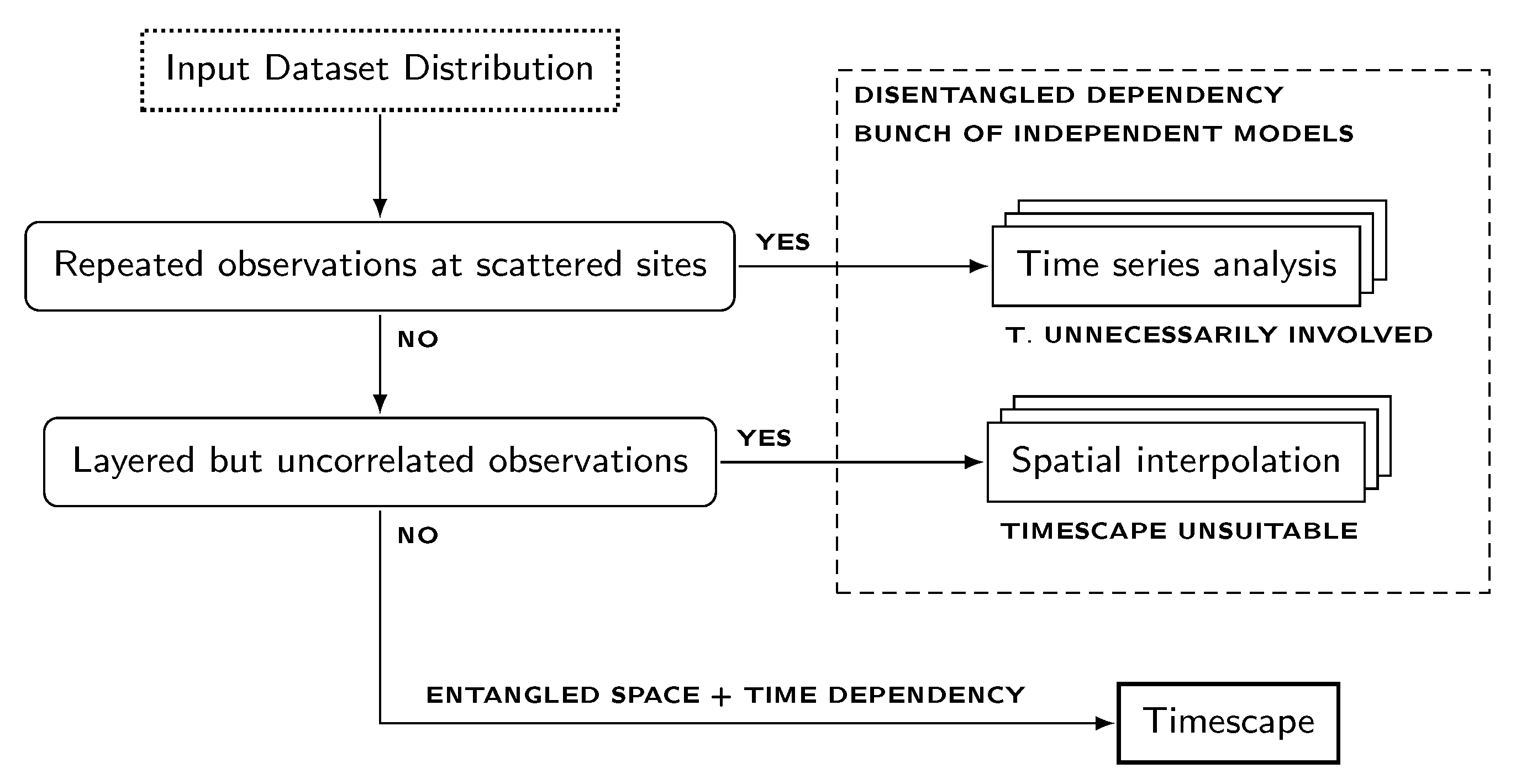
Timescape: A Novel Spatiotemporal Modeling Tool


Abstract
:1. Introduction
2. Methods
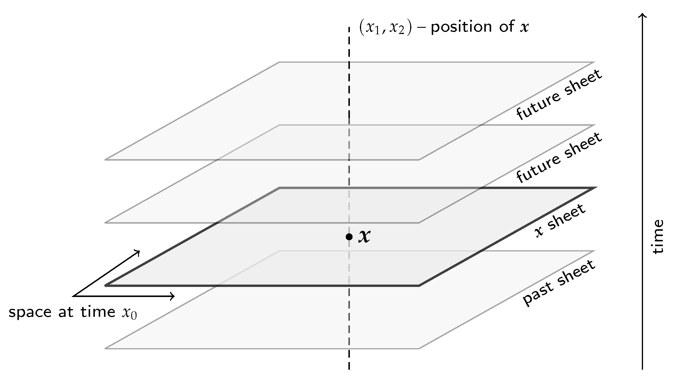
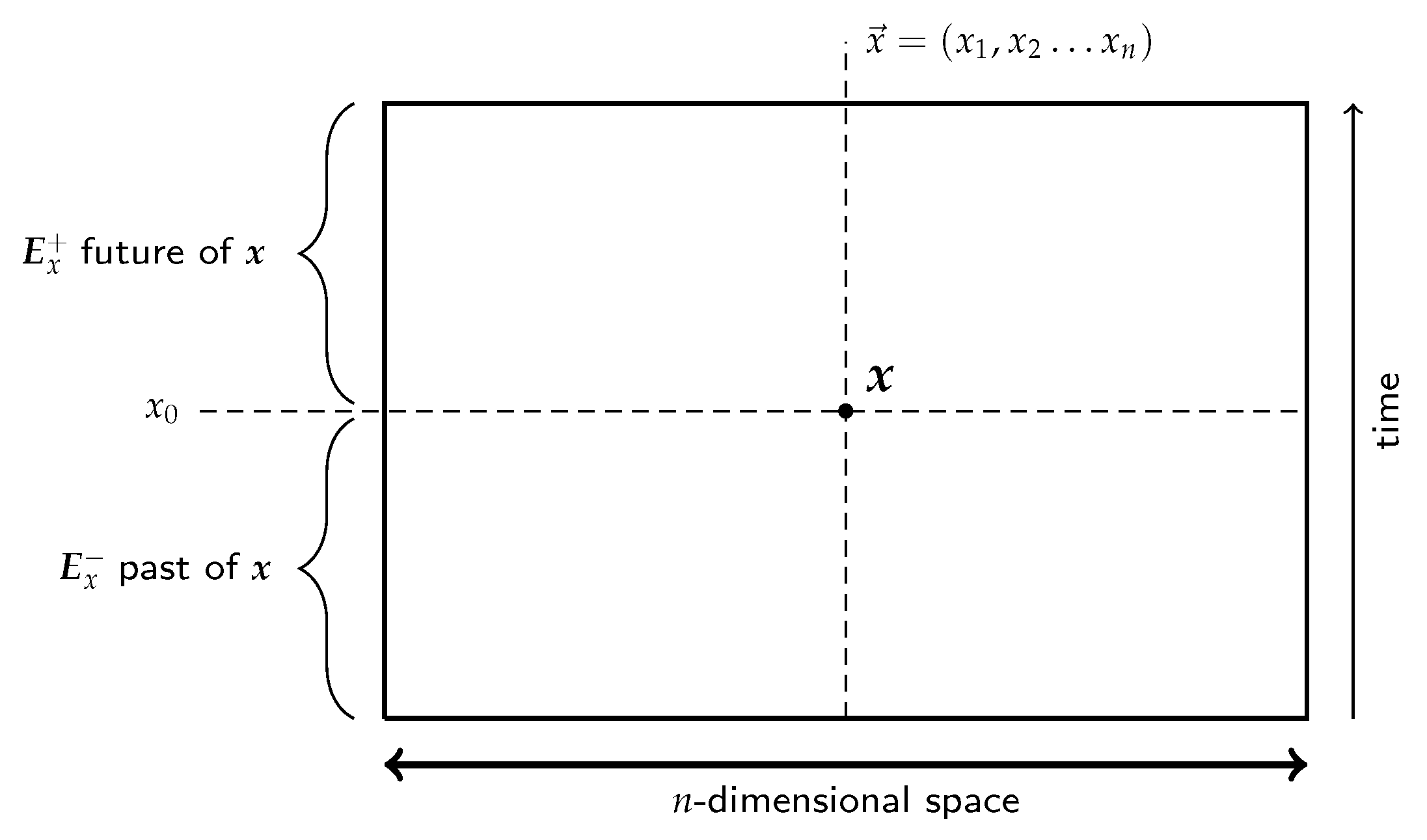
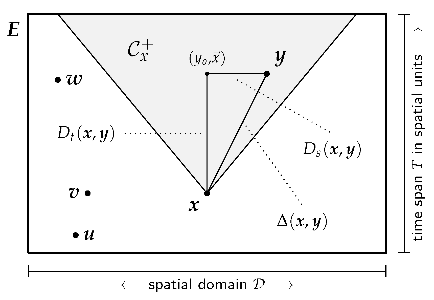
2.1. Space–Time Distances
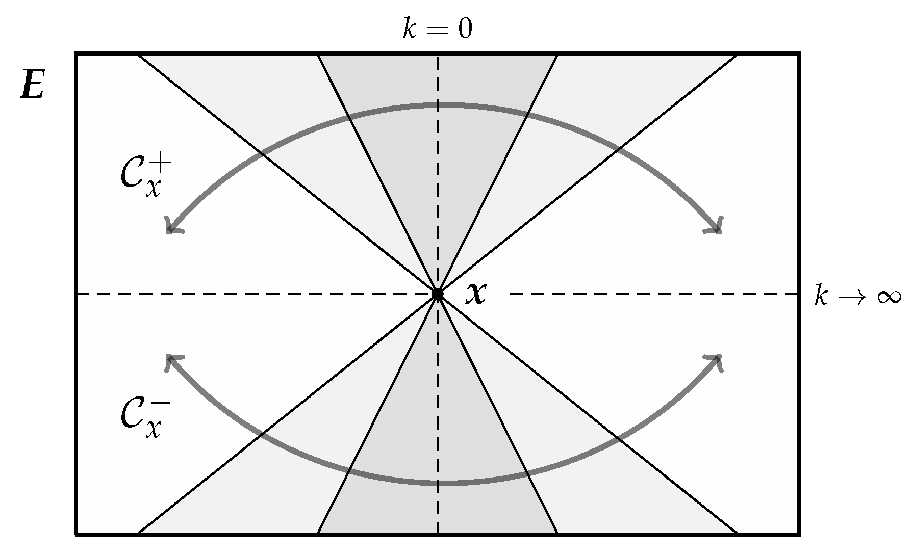
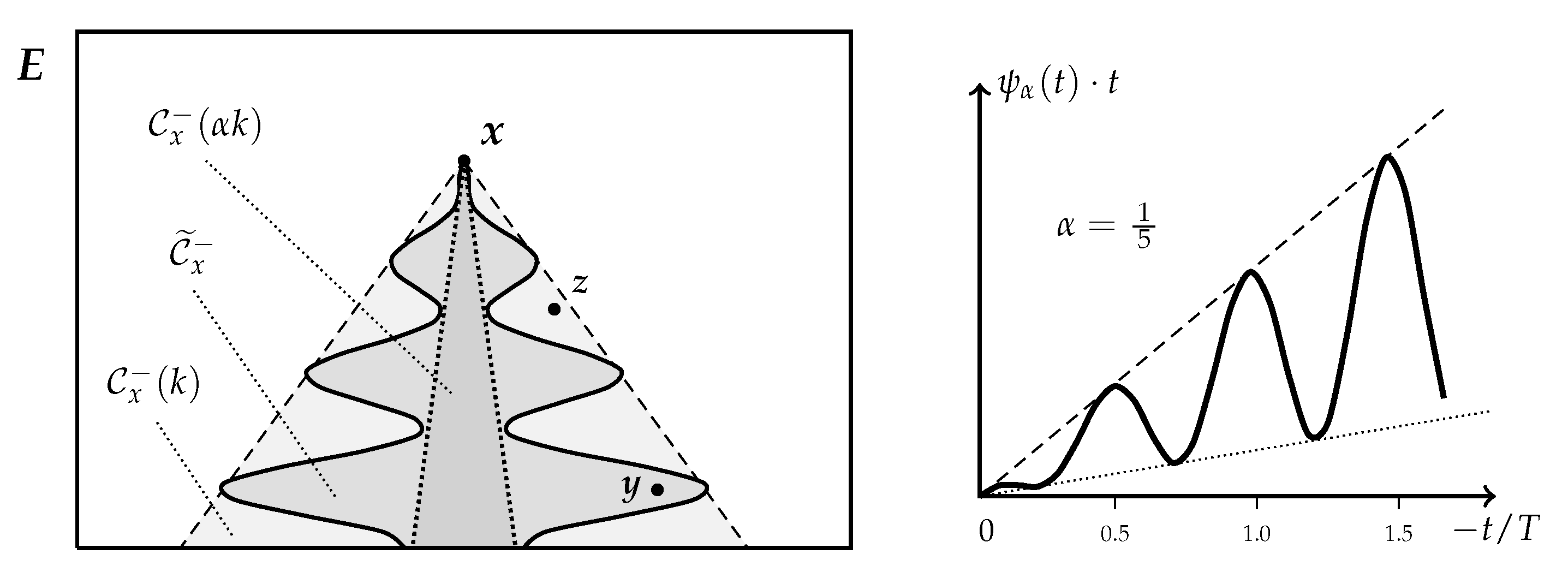
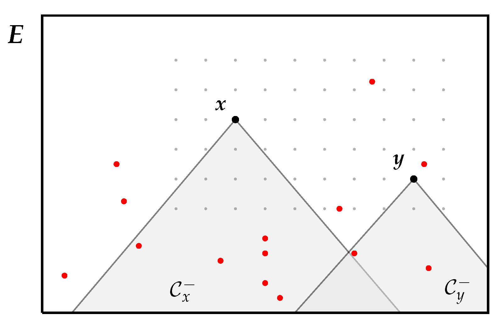
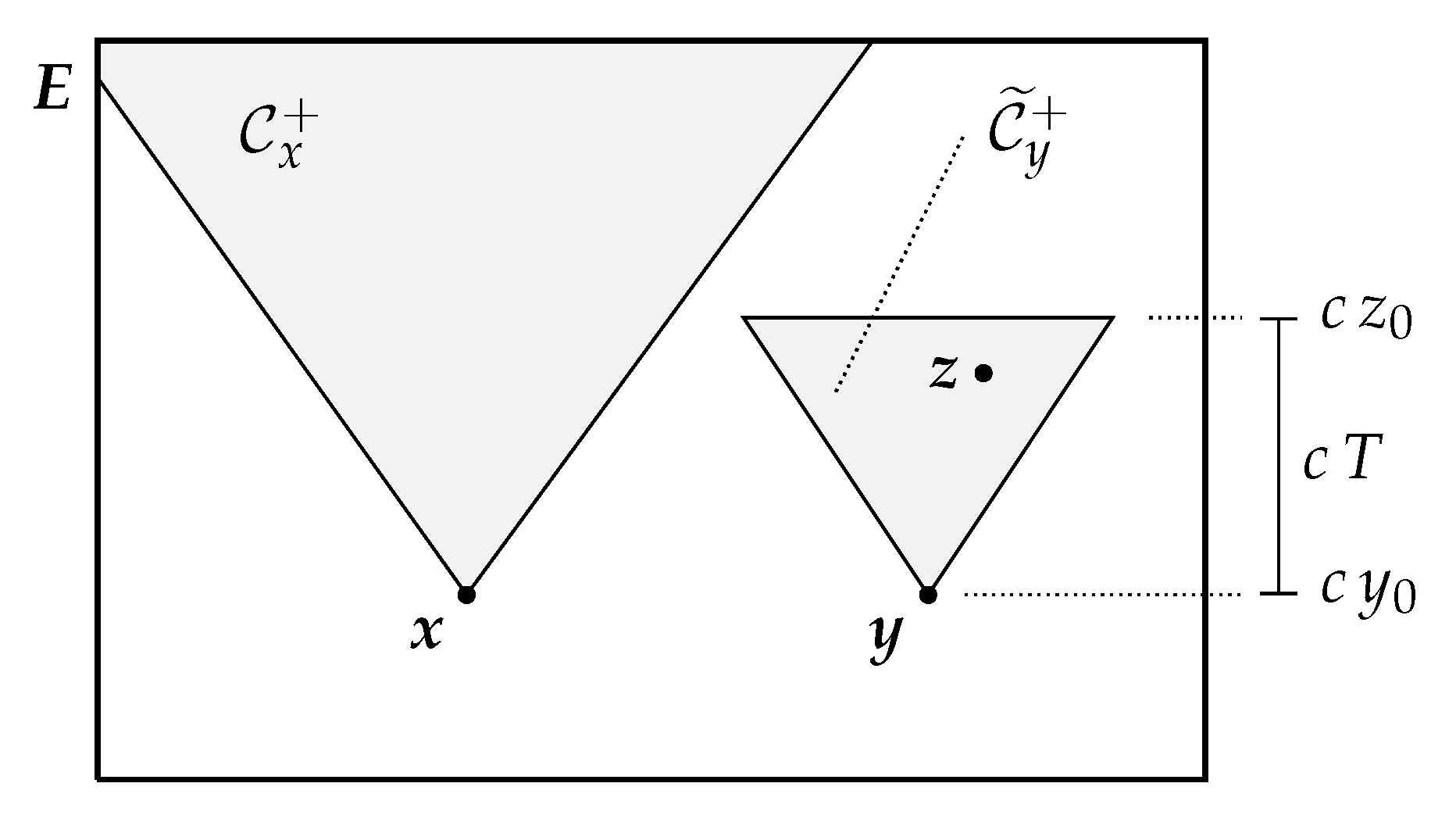
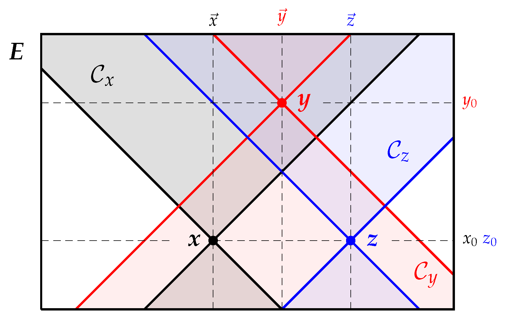
2.2. Causal Structure: Topology of the Events Space
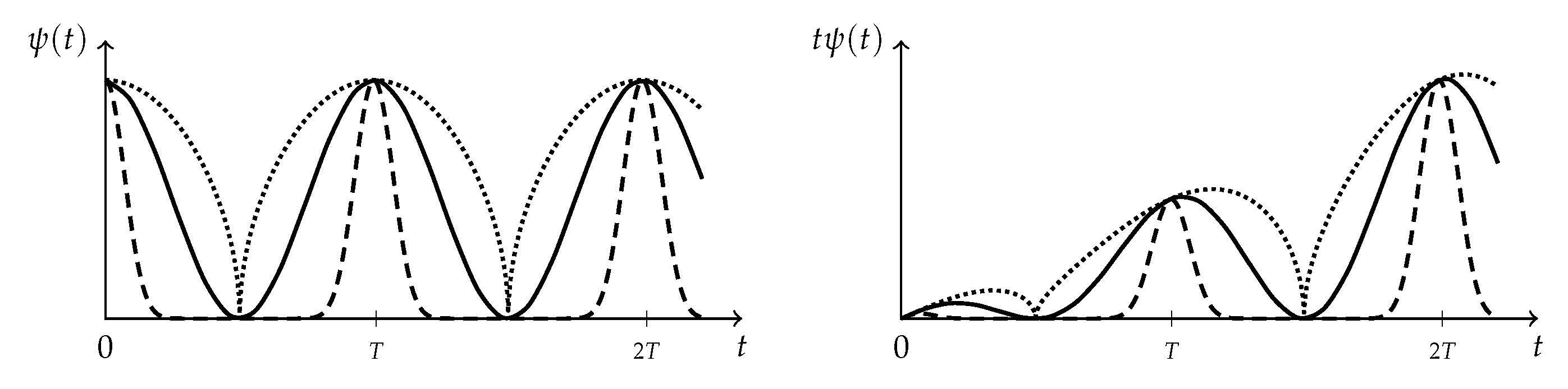
Accommodating Seasonal Variability
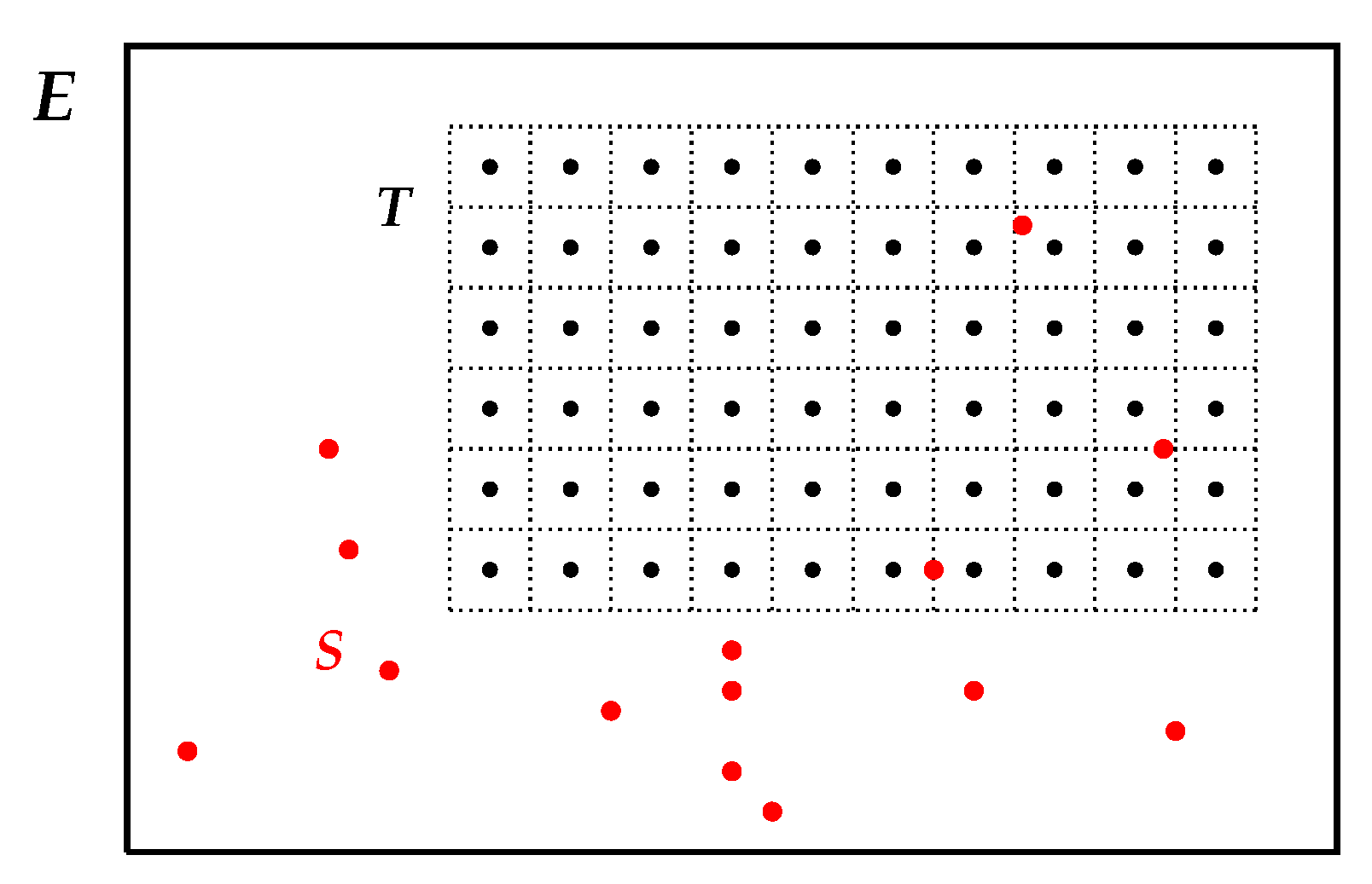
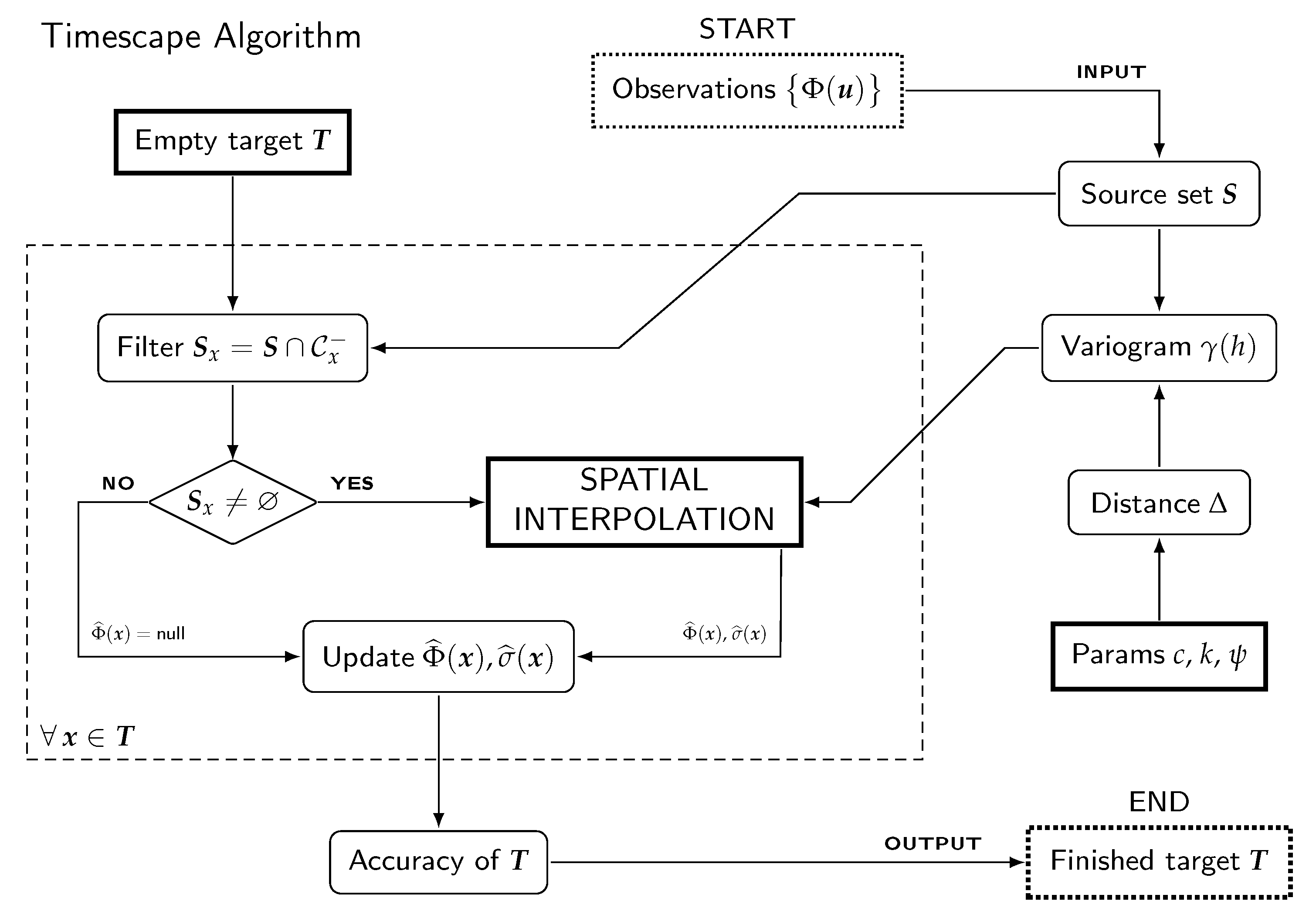
2.3. The Algorithm
2.4. Model Tuning
2.4.1. Spatial Interpolator
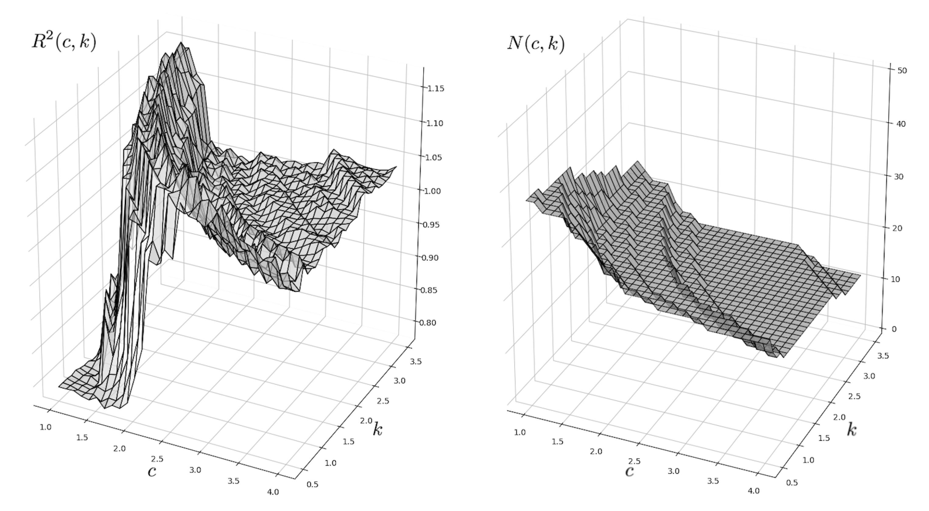
2.4.2. Metric Parameters
2.4.3. Form Factor
2.5. Timescape Implementations
2.5.1. Python
2.5.2. Java
2.6. Coping with Binary and Count Data
3. Results
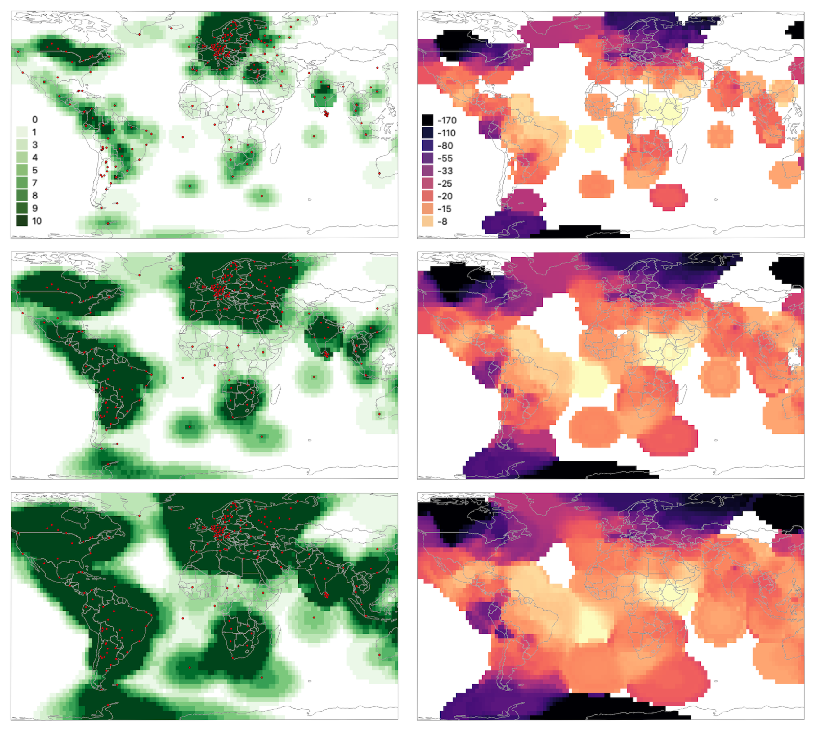
3.1. Fungi N
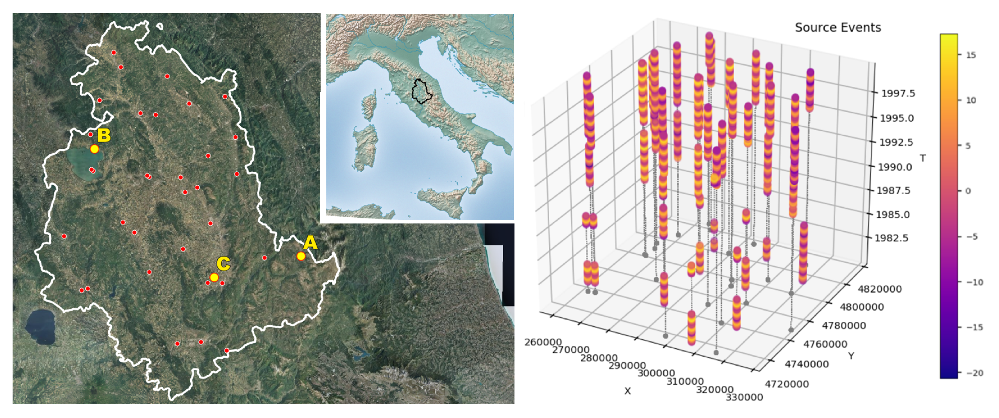
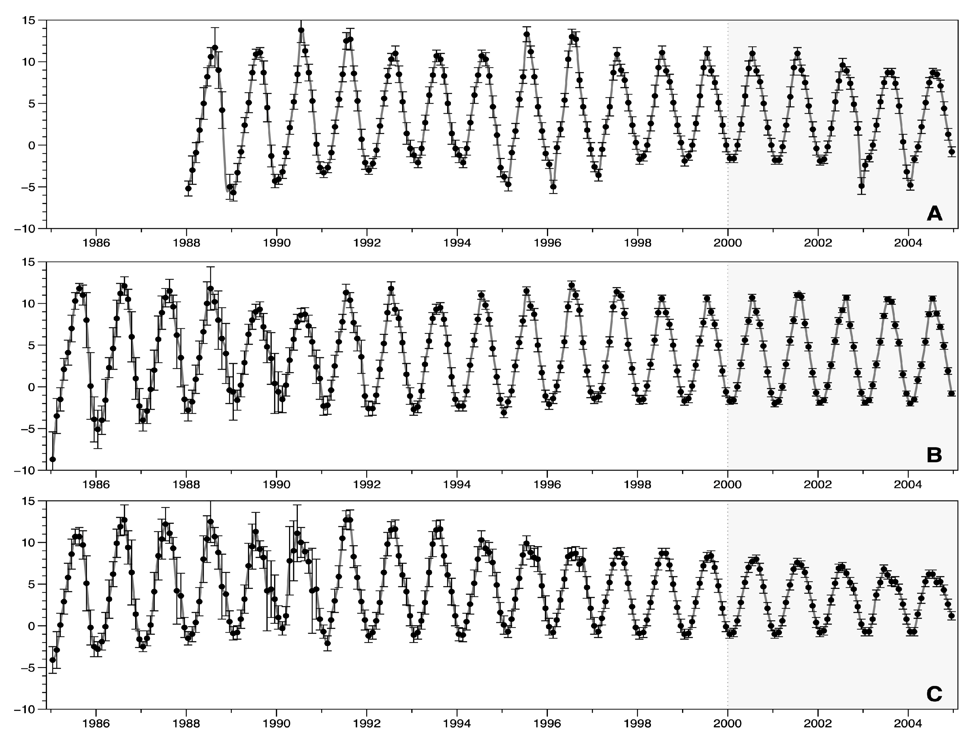
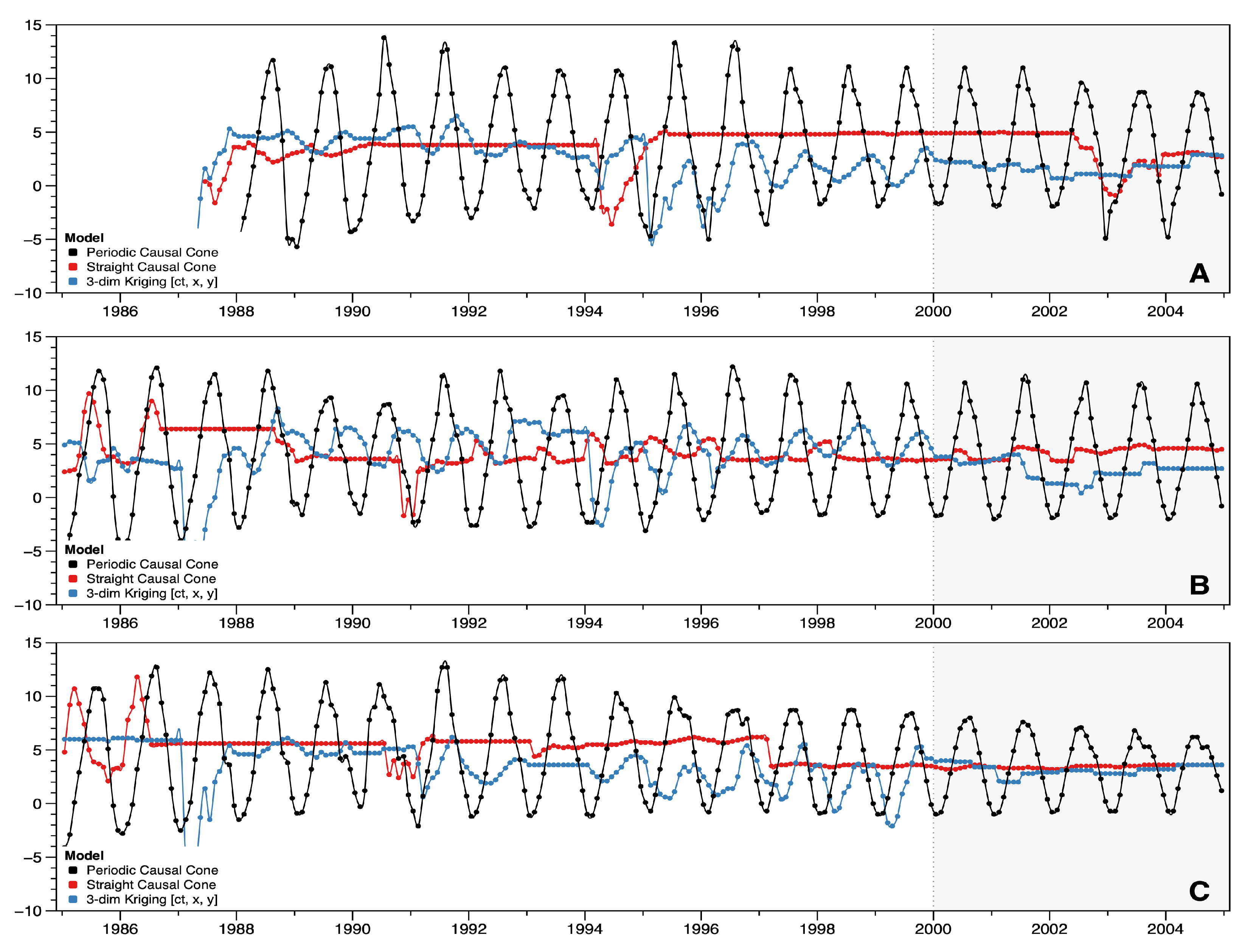
3.2. Lowest Temperatures
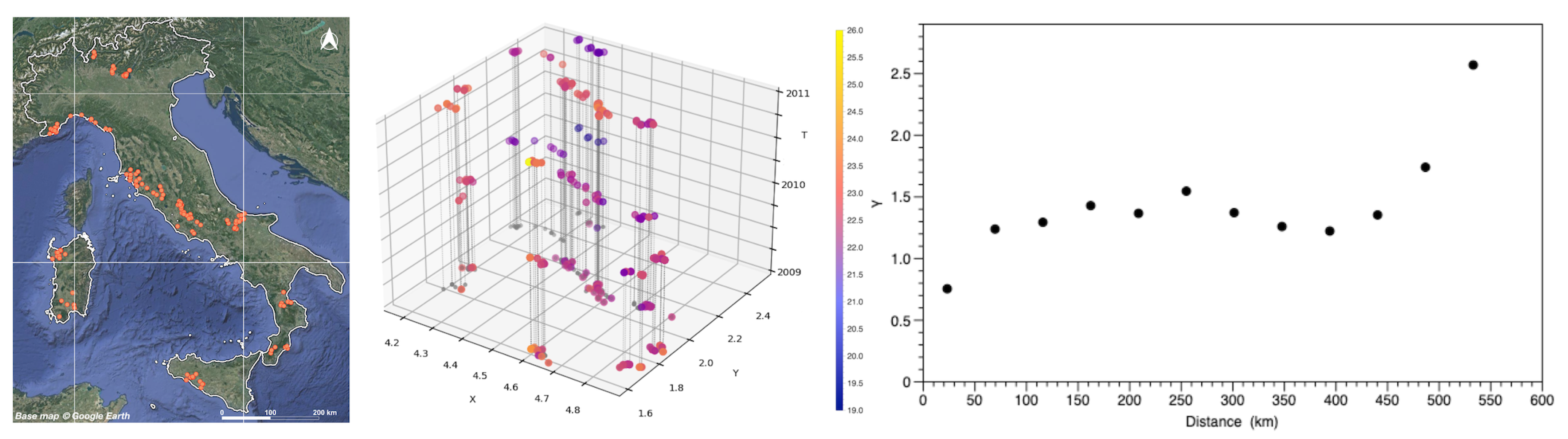
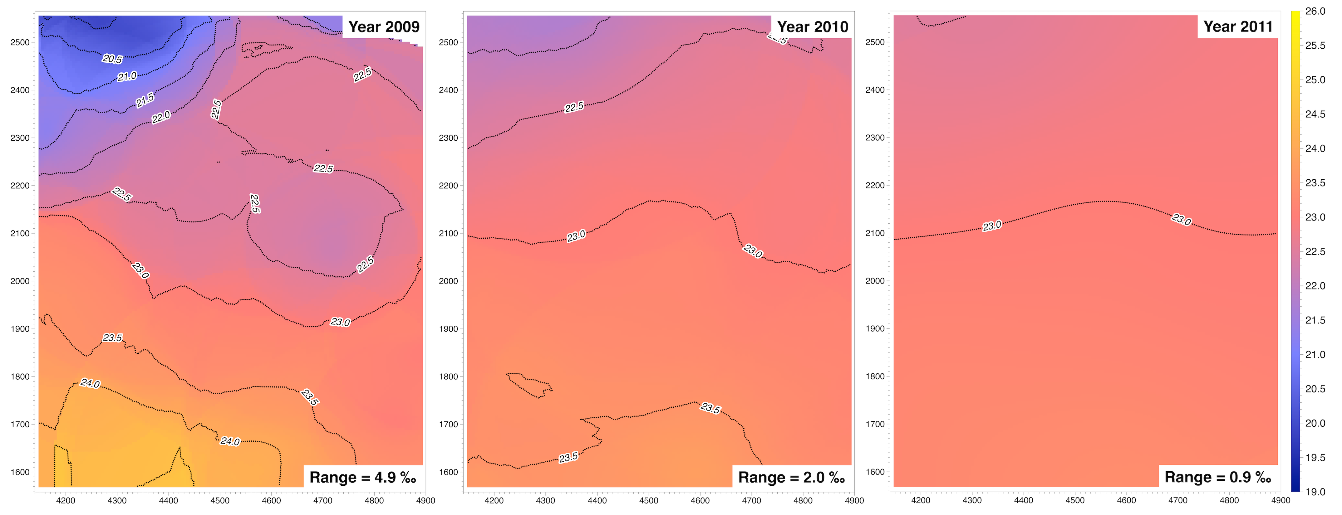
3.3. Extra Virgin Olive Oil O
3.4. Precipitation H
3.5. Performance Analysis
- -
- configuration 1: laptop–Intel i7 @ 2.60 GHz, 4 cores, 16 GByte RAM, SSD storage, Python 3.8 on Windows 10 OS.
- -
- configuration 2: laptop–Intel i7 @ 2.30 GHz, 4 cores, 8 GByte RAM, SSD storage, Python 3.7 on Ubuntu Linux 19.10 OS.
- -
- configuration 3: virtual machine–Oracle Virtualbox on MacPro host, Intel Xeon-E5 @ 3.50 GHz–4 dedicated cores, 16 GByte reserved RAM out of 64, SSD storage, Python 3.8 on Xubuntu Linux 20.04-LTS OS.
4. Discussion
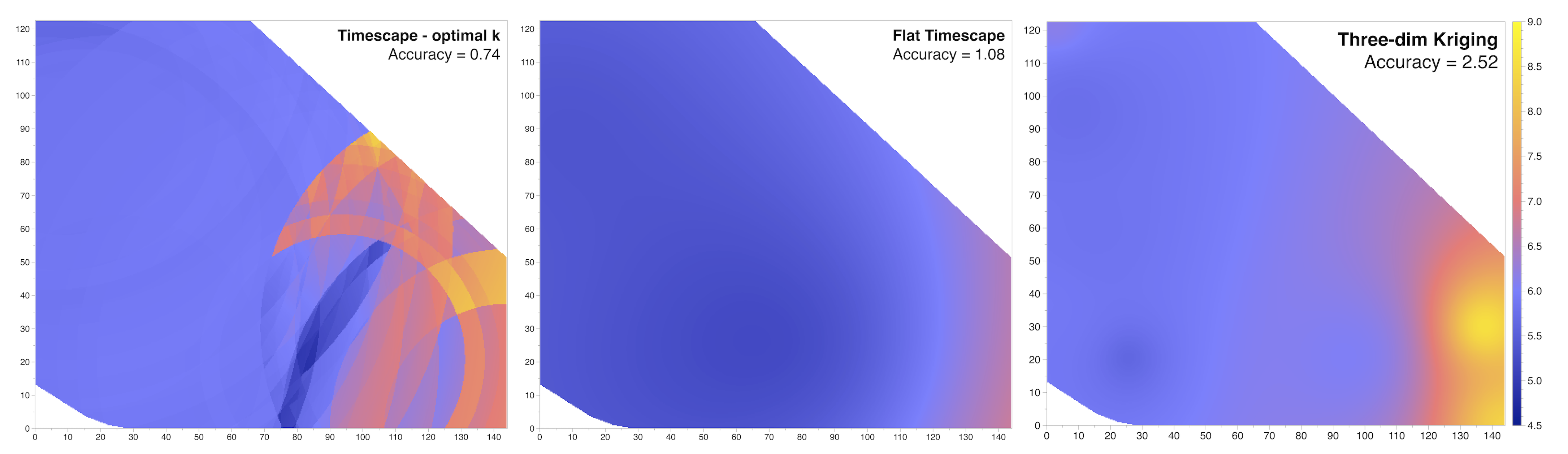
4.1. Measurements, Stationarity, Accuracy
4.2. Timescape Topology Modification
4.3. Timescape vs. Minkowskian Geometry
4.4. A Universal Tool?
5. Conclusions
Author Contributions
Funding
Institutional Review Board Statement
Informed Consent Statement
Data Availability Statement
Conflicts of Interest
References
- Evans, M.R. Modelling ecological systems in a changing world. Philos. Trans. R. Soc. B Biol. Sci. 2012, 367, 181–190. [Google Scholar] [CrossRef] [PubMed] [Green Version]
- Beran, J. Mathematical Foundations of Time Series Analysis; Springer International Publishing: Berlin/Heidelberg, Germany, 2017. [Google Scholar] [CrossRef]
- Shumway, R.H.; Stoffer, D.S. Time Series Analysis and Its Applications; Springer International Publishing: Berlin/Heidelberg, Germany, 2017. [Google Scholar] [CrossRef]
- Cressie, N. Statistics for Spatial Data; John Wiley & Sons, Inc.: Hoboken, NJ, USA, 1993. [Google Scholar] [CrossRef]
- Chilès, J.P.; Delfiner, P. Geostatistics; John Wiley & Sons, Inc.: Hoboken, NJ, USA, 2012. [Google Scholar] [CrossRef]
- Delicado, P.; Giraldo, R.; Comas, C.; Mateu, J. Statistics for spatial functional data: Some recent contributions. Environmetrics 2009, 21, 224–239. [Google Scholar] [CrossRef]
- Cressie, N.; Wikle, C.K. Statistics for Spatio-Temporal Data; John Wiley & Sons, Inc.: Hoboken, NJ, USA, 2015. [Google Scholar]
- Wikle, C.K.; Zammit-Mangion, A.; Cressie, N. Spatio-Temporal Statistics with R; Chapman and Hall/CRC: Boca Raton, FL, USA, 2019. [Google Scholar]
- Kyriakidis, P.C.; Journel, A.G. Geostatistical space-time models: A review. Math. Geol. 1999, 31, 651–684. [Google Scholar] [CrossRef]
- Le, N.D.; Zidek, J.V. Statistical Analysis of Environmental Space-Time Processes; Springer Series in Statistics; Springer: Berlin/Heidelberg, Germany, 2006. [Google Scholar]
- Epperson, B.K. Spatial and space–time correlations in ecological models. Ecol. Model. 2000, 132, 63–76. [Google Scholar] [CrossRef]
- Pebesma, E. Spacetime: Spatio-Temporal Data in R. J. Stat. Softw. 2012, 51, 1–30. [Google Scholar] [CrossRef] [Green Version]
- Graeler, B.; Pebesma, E.; Heuvelink, G. Spatio-Temporal Interpolation using gstat. R J. 2016, 8, 204–218. [Google Scholar] [CrossRef]
- R Core Team. R: A Language and Environment for Statistical Computing; R Foundation for Statistical Computing: Vienna, Austria, 2018. [Google Scholar]
- Chen, Q.; Han, R.; Ye, F.; Li, W. Spatio-temporal ecological models. Ecol. Inform. 2011, 6, 37–43. [Google Scholar] [CrossRef]
- Holmes, E.E.; Lewis, M.A.; Banks, J.E.; Veit, R.R. Partial Differential Equations in Ecology: Spatial Interactions and Population Dynamics. Ecology 1994, 75, 17–29. [Google Scholar] [CrossRef]
- Lindgren, F.; Rue, H.; Lindström, J. An explicit link between Gaussian fields and Gaussian Markov random fields: The stochastic partial differential equation approach. J. R. Stat. Soc. Ser. B (Stat. Methodol.) 2011, 73, 423–498. [Google Scholar] [CrossRef] [Green Version]
- Rue, H.; Lindgren, F.; van Niekerk, J.; Krainski, E.; Fattah, E.A. R-INLA: Approximate Bayesian Inference for Latent Gaussian Models. Available online: https://www.r-inla.org (accessed on 7 January 2022).
- Christin, S.; Hervet, É.; Lecomte, N. Applications for deep learning in ecology. Methods Ecol. Evol. 2019, 10, 1632–1644. [Google Scholar] [CrossRef]
- Brodrick, P.G.; Davies, A.B.; Asner, G.P. Uncovering Ecological Patterns with Convolutional Neural Networks. Trends Ecol. Evol. 2019, 34, 734–745. [Google Scholar] [CrossRef] [PubMed]
- Knorr-Held, L. Bayesian modeling of inseparable space-time variation in disease risk. Stat. Med. 2000, 19, 2555–2567. [Google Scholar] [CrossRef] [Green Version]
- Bolker, B.M.; Brooks, M.E.; Clark, C.J.; Geange, S.W.; Poulsen, J.R.; Stevens, M.H.H.; White, J.S.S. Generalized linear mixed models: A practical guide for ecology and evolution. Trends Ecol. Evol. 2009, 24, 127–135. [Google Scholar] [CrossRef] [PubMed]
- Elith, J.; Leathwick, J.R.; Hastie, T. A working guide to boosted regression trees. J. Anim. Ecol. 2008, 77, 802–813. [Google Scholar] [CrossRef]
- Fritsch, M.; Lischke, H.; Meyer, K.M. Scaling methods in ecological modelling. Methods Ecol. Evol. 2020, 11, 1368–1378. [Google Scholar] [CrossRef]
- Wang, J.F.; Stein, A.; Gao, B.B.; Ge, Y. A review of spatial sampling. Spat. Stat. 2012, 2, 1–14. [Google Scholar] [CrossRef]
- Jun, M.; Stein, M.L. Nonstationary covariance models for global data. Ann. Appl. Stat. 2008, 2, 1271–1289. [Google Scholar] [CrossRef]
- Frankel, T. The Geometry of Physics; Cambridge University Press: Cambridge, UK, 2009. [Google Scholar] [CrossRef]
- Jost, J. Geometry and Physics; Springer: Berlin/Heidelberg, Germany, 2009. [Google Scholar] [CrossRef]
- Ashtekar, A.; Petkov, V. (Eds.) Springer Handbook of Spacetime; Springer: Berlin/Heidelberg, Germany, 2014. [Google Scholar] [CrossRef]
- Basseville, M. Distance measures for signal processing and pattern recognition. Signal Process. 1989, 18, 349–369. [Google Scholar] [CrossRef] [Green Version]
- Ciolfi, M. Timescape Python Module, GNU-GPL 3 License. Available online: https://github.com/ciolfis/timescape (accessed on 1 December 2021).
- Ciolfi, M. TimescapeLocal Java Application, GNU-GPL 3 License. Available online: https://sourceforge.net/projects/timescapelocal (accessed on 1 December 2021).
- Ciolfi, M. TimescapeGlobal Java Application, GNU-GPL 3 License. Available online: https://sourceforge.net/projects/timescapeglobal (accessed on 1 December 2021).
- Jost, J. Riemannian Geometry and Geometric Analysis; Springer: Berlin/Heidelberg, Germany, 2011. [Google Scholar] [CrossRef]
- Banerjee, S. On Geodetic Distance Computations in Spatial Modeling. Biometrics 2005, 61, 617–625. [Google Scholar] [CrossRef]
- Mamajek, E.E.; Prsa, A.; Torres, G.; Harmanec, P.; Asplund, M.; Bennett, P.D.; Capitaine, N.; Christensen-Dalsgaard, J.; Depagne, E.; Folkner, W.M.; et al. IAU 2015 Resolution B3 on Recommended Nominal Conversion Constants for Selected Solar and Planetary Properties. arXiv 2015, arXiv:1510.07674. [Google Scholar]
- Ambartzumian, R.V. A note on pseudo-metrics on the plane. Z. Wahrscheinlichkeitstheorie Verwandte Geb. 1976, 37, 145–155. [Google Scholar] [CrossRef]
- Schroeder, V. Quasi-metric and metric spaces. Conform. Geom. Dyn. Am. Math. Soc. 2006, 10, 355–361. [Google Scholar] [CrossRef]
- Scott, D.W. On optimal and data-based histograms. Biometrika 1979, 66, 605–610. [Google Scholar] [CrossRef]
- Efron, B.; Stein, C. The Jackknife Estimate of Variance. Ann. Stat. 1981, 9, 586–596. [Google Scholar] [CrossRef]
- Knight, K. Mathematical Statistics; Chapman & Hall CRC: Boca Raton, FL, USA, 2000. [Google Scholar]
- McIntosh, A. The Jackknife Estimation Method. arXiv 2016, arXiv:1606.00497. [Google Scholar]
- Bennett, N.D.; Croke, B.F.; Guariso, G.; Guillaume, J.H.; Hamilton, S.H.; Jakeman, A.J.; Marsili-Libelli, S.; Newham, L.T.; Norton, J.P.; Perrin, C.; et al. Characterising performance of environmental models. Environ. Model. Softw. 2013, 40, 1–20. [Google Scholar] [CrossRef]
- PyKrige Developers. PyKrige, 2D and 3D Python Kriging Implementation. Available online: https://pykrige.readthedocs.io (accessed on 1 December 2021).
- Open Geospatial Consortium. OGC GeoTIFF Standard. Available online: https://www.opengeospatial.org/standards/geotiff (accessed on 1 December 2021).
- Ciolfi, M.; Chiocchini, F.; Mattioni, M.; Lauteri, M. Timescape Local spacetime interpolation tool: Projected coordinates java standalone application. Smart ELab 2017, 10, 20–39. [Google Scholar] [CrossRef]
- Ciolfi, M.; Chiocchini, F.; Mattioni, M.; Lauteri, M. Timescape Global spacetime interpolation tool: Geographic coordinates java standalone application. Smart ELab 2018, 11, 1–51. [Google Scholar] [CrossRef]
- Hibernate Object Relational Mapping. Available online: http://hibernate.org (accessed on 1 December 2021).
- Oracle. MySQL Developer Zone. Available online: https://dev.mysql.com (accessed on 1 December 2021).
- Gallant, S. Perceptron-based learning algorithms. IEEE Trans. Neural Netw. 1990, 1, 179–191. [Google Scholar] [CrossRef]
- West, J.B.; Bowen, G.J.; Dawson, T.E.; Tu, K.P. (Eds.) Isoscapes; Springer: Dordrecht, The Netherlands, 2010. [Google Scholar] [CrossRef]
- Wagner, H.H.; Fortin, M.J. Spatial Analysis of Landscapes: Concepts and Statistics. Ecology 2005, 86, 1975–1987. [Google Scholar] [CrossRef] [Green Version]
- Rossi, R.E.; Mulla, D.J.; Journel, A.G.; Franz, E.H. Geostatistical Tools for Modeling and Interpreting Ecological Spatial Dependence. Ecol. Monogr. 1992, 62, 277–314. [Google Scholar] [CrossRef]
- West, J.B.; Bowen, G.J.; Cerling, T.E.; Ehleringer, J.R. Stable isotopes as one of nature’s ecological recorders. Trends Ecol. Evol. 2006, 21, 408–414. [Google Scholar] [CrossRef] [PubMed]
- Bowen, G.J.; Good, S.P. Incorporating water isoscapes in hydrological and water resource investigations. WIREs Water 2015, 2, 107–119. [Google Scholar] [CrossRef]
- West, J.B.; Sobek, A.; Ehleringer, J.R. A Simplified GIS Approach to Modeling Global Leaf Water Isoscapes. PLoS ONE 2008, 3, e2447. [Google Scholar] [CrossRef] [PubMed] [Green Version]
- Brugnoli, E.; Farquhar, G.D. Photosynthetic Fractionation of Carbon Isotopes. In Photosynthesis; Springer: Dordrecht, The Netherlands, 2000; pp. 399–434. [Google Scholar] [CrossRef]
- Hobson, K.A.; Wassenaar, L.I. (Eds.) Tracking Animal Migration with Stable Isotopes, 2nd ed.; Elsevier: Amsterdam, The Netherlands, 2019; ISBN 9780128147238. [Google Scholar] [CrossRef]
- Chesson, L.A.; Tipple, B.J.; Ehleringer, J.R.; Park, T.; Bartelink, E.J. Forensic applications of isotope landscapes (“isoscapes”). In Forensic Anthropology; John Wiley & Sons, Ltd.: Hoboken, NJ, USA, 2017; pp. 127–148. [Google Scholar] [CrossRef]
- Bivand, R.S.; Pebesma, E.; Gomez-Rubio, V. Applied Spatial Data Analysis with R; Springer: New York, NY, USA, 2013. [Google Scholar] [CrossRef]
- Pebesma, E.; Bivand, R. Classes and Methods for Spatial Data in R. R News 2005, 5, 1–20. [Google Scholar]
- Ciolfi, M.; Piovesan, G. Spatiotemporal Analysis and Modeling of Ecological Processes at Ecosystem, Landscape and Bioregion Scale. Ph.D. Thesis, Università della Tuscia, Viterbo, Italy, 2016. [Google Scholar]
- Hogberg, P.; Hogberg, M.N.; Quist, M.E.; Ekblad, A.; Nasholm, T. Nitrogen isotope fractionation during nitrogen uptake by ectomycorrhizal and non-mycorrhizal Pinus sylvestris. New Phytol. 1999, 142, 569–576. [Google Scholar] [CrossRef]
- Hobbie, E.A.; Colpaert, J.V. Nitrogen availability and colonization by mycorrhizal fungi correlate with nitrogen isotope patterns in plants. New Phytol. 2003, 157, 115–126. [Google Scholar] [CrossRef] [PubMed]
- Dawson, T.E.; Mambelli, S.; Plamboeck, A.H.; Templer, P.H.; Tu, K.P. Stable Isotopes in Plant Ecology. Annu. Rev. Ecol. Syst. 2002, 33, 507–559. [Google Scholar] [CrossRef]
- Henn, M.R.; Chapela, I.H. Ecophysiology of 13C and 15N isotopic fractionation in forest fungi and the roots of the saprotrophic-mycorrhizal divide. Oecologia 2001, 128, 480–487. [Google Scholar] [CrossRef]
- Govindarajulu, M.; Pfeffer, P.E.; Jin, H.; Abubaker, J.; Douds, D.D.; Allen, J.W.; Bücking, H.; Lammers, P.J.; Shachar-Hill, Y. Nitrogen transfer in the arbuscular mycorrhizal symbiosis. Nature 2005, 435, 819–823. [Google Scholar] [CrossRef]
- Umbria Region Hydrographic Service. Available online: https://servizioidrografico.regione.umbria.it (accessed on 1 December 2021).
- Annali Regione Umbria. Annals of the Umbria Hydrographic Service. Available online: https://annali.regione.umbria.it (accessed on 1 December 2021).
- Natural Earth Public Domain Vector and Raster Maps. Available online: https://www.naturalearthdata.com (accessed on 1 December 2021).
- Geoportale Nazionale of the Italian Ministry for the Environment. Available online: http://www.pcn.minambiente.it (accessed on 1 December 2021).
- QGIS Development Team. QGIS Geographic Information System. Open Source Geospatial Foundation Project. Available online: http://qgis.osgeo.org (accessed on 1 December 2021).
- Giraldo, R.; Delicado, P.; Mateu, J. Continuous Time-Varying Kriging for Spatial Prediction of Functional Data: An Environmental Application. J. Agric. Biol. Environ. Stat. 2010, 15, 66–82. [Google Scholar] [CrossRef]
- Chiocchini, F.; Portarena, S.; Ciolfi, M.; Brugnoli, E.; Lauteri, M. Isoscapes of carbon and oxygen stable isotope compositions in tracing authenticity and geographical origin of Italian extra-virgin olive oils. Food Chem. 2016, 202, 291–301. [Google Scholar] [CrossRef] [PubMed] [Green Version]
- Portarena, S.; Gavrichkova, O.; Lauteri, M.; Brugnoli, E. Authentication and traceability of Italian extra-virgin olive oils by means of stable isotopes techniques. Food Chem. 2014, 164, 12–16. [Google Scholar] [CrossRef]
- Camin, F.; Larcher, R.; Nicolini, G.; Bontempo, L.; Bertoldi, D.; Perini, M.; Schlicht, C.; Schellenberg, A.; Thomas, F.; Heinrich, K.; et al. Isotopic and Elemental Data for Tracing the Origin of European Olive Oils. J. Agric. Food Chem. 2010, 58, 570–577. [Google Scholar] [CrossRef] [PubMed]
- Longinelli, A.; Selmo, E. Isotopic composition of precipitation in Italy: A first overall map. J. Hydrol. 2003, 270, 75–88. [Google Scholar] [CrossRef]
- Isotopic Composition of Precipitation in the Mediterranean Basin in Relation to Air Circulation Patterns and Climate; Number 1453 in TECDOC Series; International Atomic Energy Agency: Vienna, Austria, 2005.
- Bowen, G.J.; Revenaugh, J. Interpolating the isotopic composition of modern meteoric precipitation. Water Resour. Res. 2003, 39, 1299. [Google Scholar] [CrossRef]
- Camin, F.; Larcher, R.; Perini, M.; Bontempo, L.; Bertoldi, D.; Gagliano, G.; Nicolini, G.; Versini, G. Characterisation of authentic Italian extra-virgin olive oils by stable isotope ratios of C, O and H and mineral composition. Food Chem. 2010, 118, 901–909. [Google Scholar] [CrossRef]
- Visual Data Tools Inc. DataGraph Scientific Graphing Tool for macOS. Available online: https://www.visualdatatools.com/DataGraph/ (accessed on 7 January 2022).
- The Global Network of Isotopes in Precipitation of the International Atomic Energy Agency. Available online: https://www.iaea.org/services/networks/gnip (accessed on 1 December 2021).
- Statistical Treatment of Data on Environmental Isotopes in Precipitation; Number 331 in Technical Reports Series; International Atomic Energy Agency: Vienna, Austria, 1992.
- IAEA. International Atomic Energy Agency. Available online: https://www.iaea.org (accessed on 1 December 2021).
- Terzer, S.; Wassenaar, L.I.; Araguás-Araguás, L.J.; Aggarwal, P.K. Global isoscapes for δ18O and δ2H in precipitation: Improved prediction using regionalized climatic regression models. Hydrol. Earth Syst. Sci. 2013, 17, 4713–4728. [Google Scholar] [CrossRef]
- IsoMAP—Isoscapes Modeling, Analysis and Prediction. Available online: http://isomap.org (accessed on 1 December 2021).
- Minkowski, H. Das Relativitätsprinzip. Ann. Phys. 1915, 352, 927–938. [Google Scholar] [CrossRef] [Green Version]
- Week, B.; Nuismer, S.L.; Harmon, L.J.; Krone, S.M. A white noise approach to evolutionary ecology. J. Theor. Biol. 2021, 521, 110660. [Google Scholar] [CrossRef]
- Lucas, T.C.D. A translucent box: Interpretable machine learning in ecology. Ecol. Monogr. 2020, 90, e01422. [Google Scholar] [CrossRef]


| 1 | Equation (7) Equation (9) Figure 3 | |
| 2 | filtering–Equation (11) Figure 7 | |
| 3 | Equation (15) | |
| 4 | if | |
| else | estimate–Equation (14) | |
| if interp. allows | Kriging… | |
| else | IDW… | |
| 5 | update : |
| Model | Coordinates | ∼Scale | Time Span-Resol. | |
|---|---|---|---|---|
| Fungi N | 62 | Local Euclidean | 100 m | few days– 1 day |
| Min temperature | 2521 | WGS84 UTM33 N | 100 km | 20 years–1 month |
| Olive oil O | 275 | European Lambert | 1000 km | 3 years–1 year |
| Precipitation H | 1152 | Geographical , | km | 10 years–1 year |
| Model | Method | Distance | Form | Target Cells |
|---|---|---|---|---|
| Fungi N | Kriging | Euclidean | ||
| Min temperature | Kriging | Euclidean | Equation (10) | |
| Olive oil O | IDW | Euclidean | ||
| Precipitation H | IDW | Geodesic |
| Model | Configuration 1 | Configuration 2 | Configuration 3 | ||||
|---|---|---|---|---|---|---|---|
| Time | evt/s | Time | evt/s | Time | evt/s | ||
| Fungi N | 55% | 8732 | 200 | 1252 | 140 | 7533 | 231 |
| Min temperature | 73% | 11549 | 28 | 1186 | 27 | 7820 | 41 |
| Olive oil O | 81% | 39 | 1315 | 47 | 1091 | 35 | 1478 |
| Precipitation H | 62% | 1542 | 157 | 164 | 124 | 1121 | 176 |
| Field Dependence | Timescape | Alternatives | References |
|---|---|---|---|
| temporal only | useless | time series analysis | [2,3] |
| ODE and PDE | |||
| prev. temporal | sharp cones | dynamical systems | [16,17,88] |
| machine learning | [89] | ||
| entangled S + T | optimal suitability | stochastic PDE | [17,18] |
| covariance-based | [12] | ||
| Bayesian modeling | [21] | ||
| neural networks | [19,20] | ||
| prev. spatial | broad cones | gen. lin. models | [22] |
| regression trees | [23] | ||
| spatial only | useless | geostatistics | [4,5] |
Publisher’s Note: MDPI stays neutral with regard to jurisdictional claims in published maps and institutional affiliations. |
© 2022 by the authors. Licensee MDPI, Basel, Switzerland. This article is an open access article distributed under the terms and conditions of the Creative Commons Attribution (CC BY) license (https://creativecommons.org/licenses/by/4.0/).
Share and Cite
Ciolfi, M.; Chiocchini, F.; Pace, R.; Russo, G.; Lauteri, M. Timescape: A Novel Spatiotemporal Modeling Tool. Earth 2022, 3, 259-286. https://doi.org/10.3390/earth3010017
Ciolfi M, Chiocchini F, Pace R, Russo G, Lauteri M. Timescape: A Novel Spatiotemporal Modeling Tool. Earth. 2022; 3(1):259-286. https://doi.org/10.3390/earth3010017
Chicago/Turabian StyleCiolfi, Marco, Francesca Chiocchini, Rocco Pace, Giuseppe Russo, and Marco Lauteri. 2022. "Timescape: A Novel Spatiotemporal Modeling Tool" Earth 3, no. 1: 259-286. https://doi.org/10.3390/earth3010017
APA StyleCiolfi, M., Chiocchini, F., Pace, R., Russo, G., & Lauteri, M. (2022). Timescape: A Novel Spatiotemporal Modeling Tool. Earth, 3(1), 259-286. https://doi.org/10.3390/earth3010017