The Theoretical Approach to the Modelling of Gully Erosion in Cohesive Soil

Abstract

The stochastic gully erosion model (STOGEM) is based on a combination of deterministic mechanics and a stochastic description of the erosion control factors. The main proposition in the model is that the depth of the active surface layer of eroded cohesive soil is equal to one particle diameter, and the deposition of eroded particles is negligible. The erosion rate at the gully bed is calculated directly from the equation of the balance between driving and resistance forces acting on soil particles in flowing water using the probability density functions of stochastic variables: flow velocity, soil aggregate size and cohesion. Probability density functions of cohesion in the model vary through time and space during the erosion event due to the changes in soil composition—armoring and loosening. This theory is still far from achieving practical application, but opens up a new way for better understanding the experimental results of gully erosion and shows the direction for future investigations.

1. Introduction

Gullying is a form of linear erosion of loose and cohesive soils (and of rocks) by a concentrated water flow [1]. It is possible to classify the forms of linear erosion by their size and stage of development. The sequence of such linear forms begins with the smallest ones—the rills on the slopes. With increasing depth, the larger linear forms are ephemeral gullies [2], which are usually destroyed by plowing, followed by typical gullies. This quantitative difference in the depth causes the main qualitative difference between active typical gullies and smaller linear erosion forms—the instability of gully walls. The processes of gully bed incision and bank erosion cause the increase in gully wall inclination and soil slumping and falling of different types. These processes are typical for the first stage of gully development. Gully formation is very intensive and its geometry (length, depth, width, area, volume) is far from stable and changes rapidly [3]. The first stage lasts from 4 to 10 years in loose sands and frozen loams, and up to 100–150 years in typical agricultural landscapes [4]. The gullies cut slopes to their whole potential (possible) length during this period, and their walls eventually stabilize.

After gully wall stabilization, usually due to vegetation, gully development moves into the second stage [3]. The gully width increases slowly due to slow soil movement (creep). Slumping can still occur at the gully head, and so gully length can also slowly increase through gravitation processes and suffusion, not by fluvial erosion [5]. At this stage, the gully is transformed into a dry valley. Often sediments washed from the catchment are deposited at the dry valley’s bottom. The walls of a dry valley become more and more gentle, its depth decreases, and the dry valley is transformed to a shallow linear hollow on the slope. The formation of hollows due to sediment deposition in dry valleys takes a significant amount of time and is discovered in paleo-geographical investigations [6].

Gullies can be also classified by their position: gullies on the hillslopes, bank gullies on the valley slopes, and bottom gullies at the valley bed. Gullies can be discontinuous and continuous, differing by soils and type of vegetation on gully slopes [7].

Mathematical models of different levels of simplification [7,8,9,10] describe all of the abovementioned forms, stages and processes. All of these models represent significant empirical components in process description. The goal of the current paper is to formulate the general theoretical principles of only one, but the main, process of gully development in cohesive soil—erosion by water. The main approach is a stochastic description of the synergy of the main destructive and stabilizing forces, which causes soil particle detachment.

2. Materials and Methods

2.1. Gully Erosion by Water

The rate of gully incision is controlled by water flow velocity, depth, turbulence, temperature, as well as soil texture, soil mechanical pattern, and the level of protection by vegetation. These characteristics are described by equations of mass conservation:

$$\frac{\partial Q_s}{\partial X}=C_w{q}_w+EW+E_{b}d-C{U}_{f}W$$

(1)

where Q_s = Q C is the sediment transport rate (m³ s⁻¹), Q is the water discharge (m³ s⁻¹); X is the longitudinal co-ordinate (m); C is the mean volumetric sediment concentration; C_w is the sediment concentration of the lateral input; q_w is the specific lateral discharge (m² s⁻¹); E is the erosion rate or the mean particle detachment rate (m s⁻¹); E_b—bank erosion rate (m s⁻¹); W is the flow width (m); d is the bank height (m); and U_f is the sediment particles’ falling velocity in the turbulent flow (m s⁻¹).

During the first stage of gully development in cohesive soil, the accumulation on the gully bed of soil particles, eroded inside the gully or from the lateral input, is usually negligible. Flow velocity of erosion initiation in cohesive soils is higher than the critical flow velocity when the settling of detached particles occurs. The rate of bank erosion E_b is related to the rate of erosion E of the gully bed [10]. Therefore, the main term in Equation (1) is the erosion rate E.

The soil erosion rate E is the mean rate of the lowering of the soil surface Z₀ or the increase in volume ΔV eroded from the area S during the time interval T.

$$E=\frac{\Delta Z_0}{T}=\frac{\Delta V}{ST}$$

(2)

The erosion volume ΔV is the sum of the volumes of individual eroded soil particles (aggregates) V_ai with correction on soil porosity ε:

$$\Delta V=\frac{1}{1-\epsilon }{\displaystyle \sum }_{i=1}^m{V}_{ai}$$

(3)

After multiplying and dividing each component of the sum (3) by the product of the soil particle bottom area s_i and the duration of particle detachment τ_i, Formula (2) takes the form:

$$E=\frac{1}{1-\epsilon }{\displaystyle \sum }_{i=1}^m\frac{V_{ai}}{s_i{\tau }_i}\frac{s_i{\tau }_i}{ST}$$

(4)

where the term V_ai/s_iτ_i represents the instant and local rate of particle detachment α, and the term s_iτ_i/ST represents the probability density of this particle detachment. Therefore [11]:

$$E=\frac{1}{1-\epsilon }{{\displaystyle \int }}_{\alpha }^{}\alpha p_{\alpha }\mathrm{d}\alpha$$

(5)

where p_α is the spatial-temporal probability density function (PDF) for α. Equations (4) and (5) show that the mean soil erosion rate is the result of spatial (on the area S) and temporal (during the period T) averaging of instant and local detachment rates α. The detachment rate α possess all positive values, including zero (“detachment” of stable particles).

2.2. Instant and Local Rate of Soil Particle Detachment

Erosion of cohesive soil is a rather slow process, even in gullies, as water mainly only comes into contact with, and thus only affects, the surface layer. The main proposition in the further consideration in this paper is that the depth of the active surface layer equals one particle diameter. The instant and local detachment is a discrete process: the surface becomes lower when and where a soil fragment is detached. A soil fragment becomes unstable, and its movement begins when and where the driving forces F_dr exceed the maximum of the resisting forces F_res and the resultant force Θ is more than zero [12]:

$$\mathsf{\Theta }=\left(\left|F_{dr}\right|-\left|F_{res}\right|\right)>0$$

(6)

The acceleration of such an unstable fragment within the soil surface layer in the direction of the resultant force Θ (along the axis Z) is described by Newton’s second law:

$$V_a{\rho }_s\frac{{\mathrm{d}}^{2}Z}{\mathrm{d}{\tau }^2}=\mathsf{\Theta }$$

(7)

where ρ_s is soil density.

A soil fragment becomes detached when all links between particles are broken, i.e., when the soil fragment is removed from its initial position by a distance greater than its height D. The duration of detachment equals.

$$\tau =\sqrt{\frac{2{\rho }_s{V}_{a}D}{\mathsf{\Theta }}}$$

(8)

The local and instant (average for the period τ) detachment rate is

$$\alpha =\frac{D}{\tau }=\sqrt{\frac{D\mathsf{\Theta }}{2{\rho }_s{V}_a}}$$

(9)

Equations (8) and (9) are valid for the simplest case when Θ is independent of Z.

Equations (8) and (9) describe the behavior of a single soil particle. It is evident that is impossible in general to predict the exact force balance or to foresee the geometry and mass of a soil particle or aggregate at a given point at a given time. The main variables in these equations are of a stochastic nature. Therefore, it is possible to describe these variables with probability density functions and use these functions to calculate the mean rate of detachment (erosion rate) with Equations (5) and (9) [13].

2.3. Probability Density Function for the Rate of Detachment

The detachment rate calculated with Equation (9) is the function of multiple factors: soil particle geometry and density, as well as driving and resistance forces. Each of these factors (often compound) is a stochastic variable characterized by a probability density function (PDF). To obtain the PDF for the function of random variables (in our case, for the particle detachment rate), it is necessary to use the appropriate calculation techniques. The main technique is the formula for calculating the mean E(Y) of a function of random variables Y = g(x₁, x₂, … x_n) [14]:

$$E\left(Y\right)=E\left[g\left(x_1,\dots x_n\right)\right]={\displaystyle \int }\dots {\displaystyle \int }g\left(x_1,\dots x_n\right)p\left(x_1,\dots x_n,\right)d{x}_1,\dots d{x}_n$$

(10)

For independent variables, the multivariable PDF p(x₁, … x_n) is equal to the product of the PDFs of each of the random variables.

2.4. The Main Resistance and Driving Forces

The process of a single particle’s detachment from the surface of cohesive soil caused by water was described in detail by Mirtskhulava [15]. We shall follow this work with additions.

The main resistance forces are: submerged weight of soil fragments, with slope inclination γ taken into account, projected in the direction of driving forces β:

$$F_w=g{V}_a\left({\rho }_s-\rho \right)\cos \gamma \sin \beta$$

(11)

and the geo-mechanical force of cohesion:

$$F_C=C{S}_b$$

(12)

The latter is a combination of electro-chemical, capillary and friction forces, which is parameterized by the product of cohesion C (in terms of Coulomb law) and contact area between and within soil aggregates S_b.

Hydrodynamic driving forces are the gradients of static and dynamic pressure, acting on the soil surface, depending on geometry of the soil surface, the shape and size of soil aggregates, the flow depth and the velocity distribution. The field of these gradients can be calculated with 3D hydrodynamic models. More often [15], these pressure gradients are calculated with the use of flow velocity and aggregates geometry as drag (F_d) and lift (F_l) forces, which are parameterizations of longitudinal and vertical pressure gradients:

$$F_d=C_R\rho S_d\frac{U^2}{2}$$

(13)

$$F_l=C_y\rho S_a\frac{U^2}{2}$$

(14)

where C_R is the coefficient of drag resistance; C_y is the coefficient of uplift; U is the instant near-bed flow velocity; ρ_s and ρ are the soil aggregate density and water density, respectively; S_d is the area of aggregate cross-section exposed perpendicular to flow; and S_a is the cross-section area of the soil aggregate parallel to the flow (vertical projection). The direction of the sum of drag and lift forces (the angle with the mean soil surface) is:

$$\beta =\arctan \frac{C_y{S}_a}{C_R{S}_d}$$

(15)

With this parametrization, the local detachment rate is [13] (with modification):

$$\begin{gathered} \alpha =\sqrt{\frac{D\mathsf{\Theta }}{2{\rho }_s{V}_a}}=\sqrt{\frac{D}{2{\rho }_s{V}_a}\left[\left(C_y\rho S_a+C_R\rho S_d\right)\frac{U^2}{2}-g\left({\rho }_s-\rho \right)V_a\cos \gamma \sin \beta -C{S}_b\right]} \\ \alpha =\sqrt{k_U{U}^2-k_{D}D-k_{C}C} \end{gathered}$$

(16)

where k_U is $\frac{\rho D}{4{\rho }_s{V}_a}\left(S_a{C}_y+S_d{C}_R\right)$, k_D is $\frac{g\left({\rho }_s-\rho \right)}{2{\rho }_s}\cos \gamma \sin \beta$ and k_C = $\frac{D{S}_b}{2{\rho }_s{V}_a}$. If the expression under the square root is equal to zero or negative, then α = 0. For this case, Equation (16) is a generalized form (with cohesion) of a well-known expression for incipient motion criteria (see, for example, [16]).

The rate of detachment is the stochastic variable, which is the function of six other independent stochastic variables: flow velocity, particle (aggregate) size, soil cohesion and three geometric-kinematical coefficients k_U, k_D and k_C. In the case of turbulent flow, C_y, C_R and k_U are constants [15]. If we assume a simple shape and composition of soil particles (aggregates), then the coefficient k_D is also constant. Then, Equation (16) contains three independent stochastic variables: flow velocity U, soil particle size D and force of cohesion k_CC, and Equation (10) takes the form:

$$E=\frac{1}{1-\epsilon }{{\displaystyle \int }}_{Cmin}^{Cmax}p\left(k_{C}C\right)\mathrm{d}{k}_{C}C{{\displaystyle \int }}_{Umin}^{Umax}p\left(\sqrt{k_U}U\right)\mathrm{d}\sqrt{k_U}U{{\displaystyle \int }}_{Dmin}^{Dmax}p\left(k_{D}D\right)\mathrm{d}{k}_{D}D\sqrt{k_U{U}^2-k_{D}D-k_{C}C}$$

(17)

where p(√k_UU), p(k_DD) and p(k_CC) are probability density functions for flow velocity, soil particles vertical size and cohesion, respectively. In numerical calculations, the continuous quantities are replaced by discrete one, infinitesimal by finite, and integrals by sums: ${{\displaystyle \int }}_{Xmin}^{Xmax}X\mathrm{d}X\to \Delta X{\displaystyle \sum }_{iX=1}^{nX}{X}_{iX}$.

2.5. Probability Density Function for the Factors of Soil Erosion

When geometric–kinematical coefficients and PDFs for flow velocity, soil aggregate size and cohesion are known from the theory or experiment, the PDF for instant and local erosion rate α and, therefore, the mean rate of erosion can be calculated with Equation (17). Various combinations of the input mean values of the factors, as well as different PDFs, lead to a great variability of the resulting relationships between erosion and controlling factors.

Measurements in different environments show [7,10,17] that the flows in the gullies are usually shallow, turbulent and often supercritical. A large number of measurements of turbulent characteristics using different techniques in such shallow flows [18,19] showed Gaussian PDF of fluctuations of instant longitudinal velocity U:

$$p\left(U\right)=\frac{1}{\sigma \sqrt{2\pi }}\exp \left[-\frac{1}{2}{\left(\frac{U-U_{mean}}{\sigma }\right)}^2\right]$$

(18)

where U_mean is the mean velocity and σ is the standard deviation of velocity fluctuations. For small mean velocities, the function p(U) can be asymmetrical.

The ratio of the standard deviation of velocities and kinematic velocity U_* increases from the flow surface to the bottom [19];

$$\frac{\sigma }{U_{*}}=2.3\exp \left(-\frac{z}{H}\right)$$

(19)

where H is the flow depth and z equals the roughness height. According to Mirtskhulava [15], in shallow turbulent flow C_y = 0.1 and C_R = 0.42; then k_U = $\left(0.1S_a+0.42S_d\right)$.

The PDF of the aggregate diameters can be expressed as a lognormal distribution [20,21]:

$$p=\frac{1}{D{\sigma }_L\sqrt{2\pi }}\exp \left[-\frac{{\left(\ln D-D_L\right)}^2}{2{\sigma }_L^2}\right]$$

(20)

The parameters in Equation (20), calculated with arithmetical values, namely the mean of soil particle height D_m and standard deviation σ_D, are

$$D_L=\ln \left(\frac{D_m^2}{\sqrt{D_m^2+{\sigma }_D^2}}\right)$$

(21)

$${\sigma }_L=\sqrt{\ln \left[1+{\left(\frac{{\sigma }_D}{D_m}\right)}^2\right]}$$

(22)

The direction of sum of drag and lift forces is $\beta =\arctan \left(0.238\frac{S_a}{S_d}\right)$, therefore k_D=$\cos \mathsf{\gamma }\frac{g\left({\rho }_s-\rho \right)}{2{\rho }_s}\sin \left[\arctan \left(0.238\frac{S_a}{S_d}\right)\right]$.

The details of the influence of soil cohesion on erosion rate are not properly investigated. Mean values, measured with existing techniques, such as tore-vane and penetrometers of different kinds, are not well correlated with aggregate stability tests and measured rates of soil erosion (see the results of experiments in [22]). Even less is known about PDFs of aggregates cohesion. Mirtskhulava [15] determined a normal distribution function for the variability of soil cohesion, measured by a round stamp. The same PDF fit to the textural tensile strength of one hundred 2–3 mm rounded aggregates [23], but the initial data, published there, show a distinct asymmetrical distribution. Our experiments, with the cutting of the surface of soil sample with a blade [24], showed the lognormal distribution of soil strength (Equation (20)). We shall use lognormal distribution in further calculations, keeping in mind that this distribution changes over time during an erosion event.

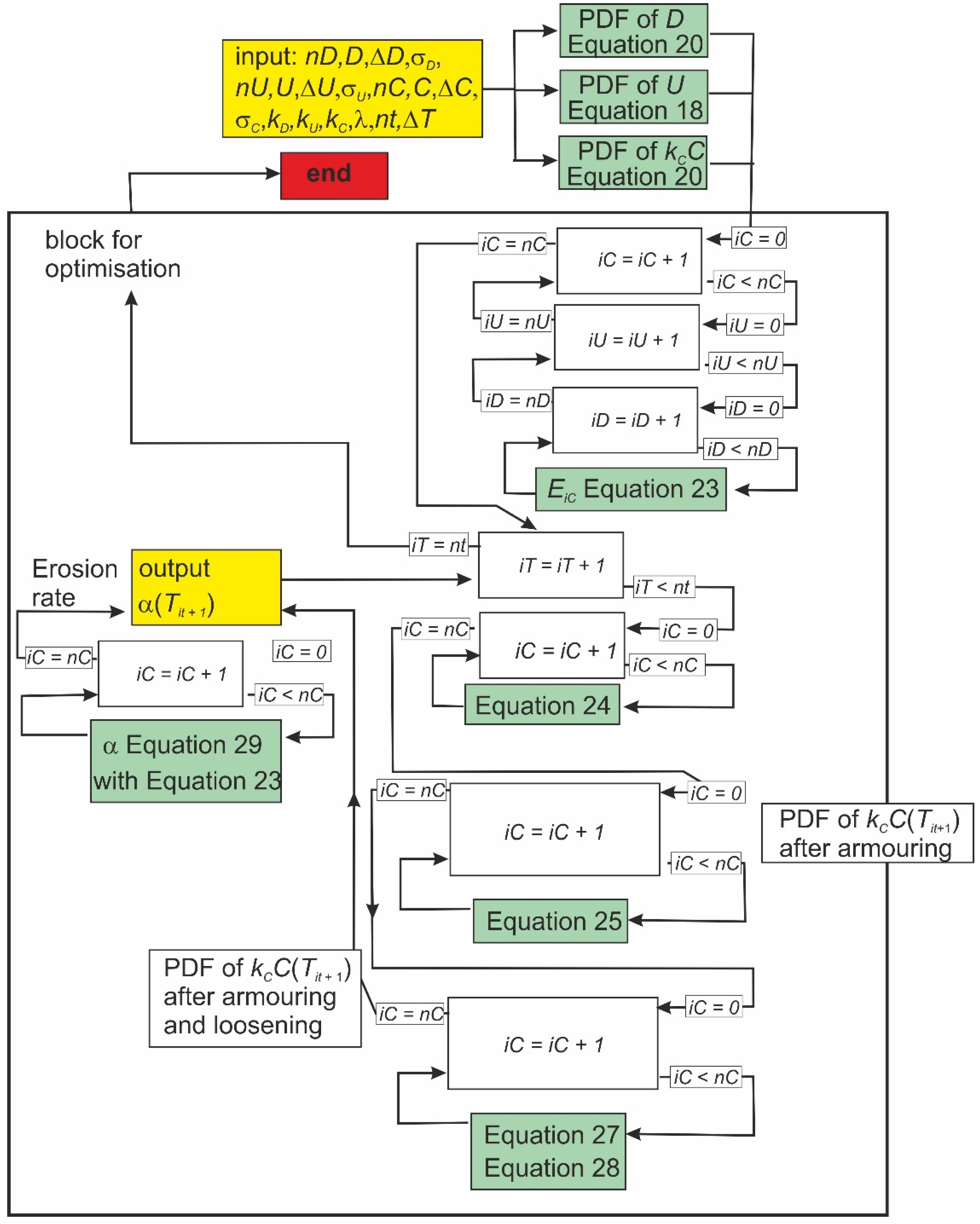
2.6. The Algorithm of Erosion Rate Calculation

Two opposite processes transform the initial spatial distribution of soil cohesion: soil armoring and soil loosening (Figure 1). The armoring due to the removal of unstable soil particles and aggregates leads to the following transformation of cohesion PDF through time:

• The probability density p(k_CC) in the part of the cohesion PDF where resistance forces are less than driving forces decreases due to the erosion E_iC of soil with particular cohesion C_iC

  $$E_{iC}=\frac{1}{1-\epsilon }{{\displaystyle \int }}_{Umin}^{Umax}p\left(\sqrt{k_U}U\right)\mathrm{d}\sqrt{k_U}U{{\displaystyle \int }}_{Dmin}^{Dmax}p\left(k_{D}D\right)\mathrm{d}{k}_{D}D\sqrt{k_U{U}^2-k_{D}D-k_{C}C}$$

  (23)
  The initial PDF transforms into intermediate PDF (p*)

  $$p^{*}\left[{\left(k_{C}C\right)}_{iC},t_{i+1}\right]\mathrm{d}{k}_{C}C=p\left[{\left(k_{C}C\right)}_{iC},t_{i+1}\right]\mathrm{d}{k}_{C}C\left[1-\frac{E_{iC}}{D_m}\left(t_{i+1}-t_i\right)\right]$$

  (24)
• Simultaneously, the intermediate PDF of cohesion is transformed due to the exposition of fresh initial soil in the “windows” of the eroded surface layer to PDF of armored soil (p_a)

$$p_a\left[{\left(k_{C}C\right)}_{iC},t_{i+1}\right]=p^{*}\left[{\left(k_{C}C\right)}_{iC},t_{i+1}\right]+p_0\left(k_{C}C\right)\left({{\displaystyle \int }}_{C_{min}}^{C_{max}}{p}_0\left(k_{C}C\right)\mathrm{d}{k}_{C}C-{{\displaystyle \int }}_{C_{min}}^{C_{max}}{p}^{*}\left[{\left(k_{C}C\right)}_{iC},t_{i+1}\right]\mathrm{d}{k}_{C}C\right)$$

(25)

where the index ‘iC’ indicates a particular soil cohesion and related erosion rate, the index ‘í’ indicates a sequence in time, and p₀($k_C$C) is the PDF of cohesion in the initial soil. This process leads to the increase in the proportion of the surface covered by stable soil aggregates, and an increase in the mean soil cohesion. The rate of erosion decreases through time when armoring is the prevailing process.

Soil loosening takes place due to the destabilization of stable aggregates when links between and/or within soil aggregates are weakening. This is complicated process, including decrease of electro-chemical, capillary and friction forces in saturated soil, the removal by flow of unstable soil particles and aggregates, which previously stabilized other aggregates, the widening of pores and cracks due to changes in water pressure in soil. Destabilization also occurs due to the vibration of stable aggregates caused by turbulent flow [15].

The failure of links decreases the contact surface area S_b between and within soil aggregates over time. The rate of failure of links in soils can be described with the common exponential failure function [25].

$$\frac{\mathrm{d}{S}_b}{\mathrm{d}t}=\lambda S_b$$

(26)

The parameter λ > 0 must be estimated from experiments.

The remaining contact area at time T_i+1 is the product of the contact area at time T_i and the failure function (Equation (26))

$$k_C\left(T_{i+1}\right)=k_C\left(T_i\right)\left[1-\lambda \mathrm{d}T\right]$$

(27)

Loosening leads to an increase in the proportion of the surface covered by unstable soil aggregates, and leads to a decrease in the mean soil cohesion. The rate of erosion increases through time when loosening occurs at a higher rate than soil armoring. Soil loosening is the main cause of erosion at the final stage of the erosion event, when the soil surface is nearly completely stabilized by armoring.

The final PDF of cohesion after the armoring and loosening cycle, as the PDF of function (27) [14], is equal to:

$$p\left[{\left(k_{C}C\right)}_{iC},T_{i+1}\right]=\frac{1}{1-\lambda \mathrm{d}T}{p}_a\left[{\left(k_{C}C\right)}_{iC},T_i\right]$$

(28)

The rate of gully erosion at a given moment is calculated from the equation of the balance between the driving and resistance forces acting on a soil particle in flowing water (Equation (17)) after soil armoring and after soil loosening (Figure 1). The armoring–loosening cycle exists only in the numerical representation of the process of erosion. In reality, soil armoring and loosening is a unified and simultaneous process.

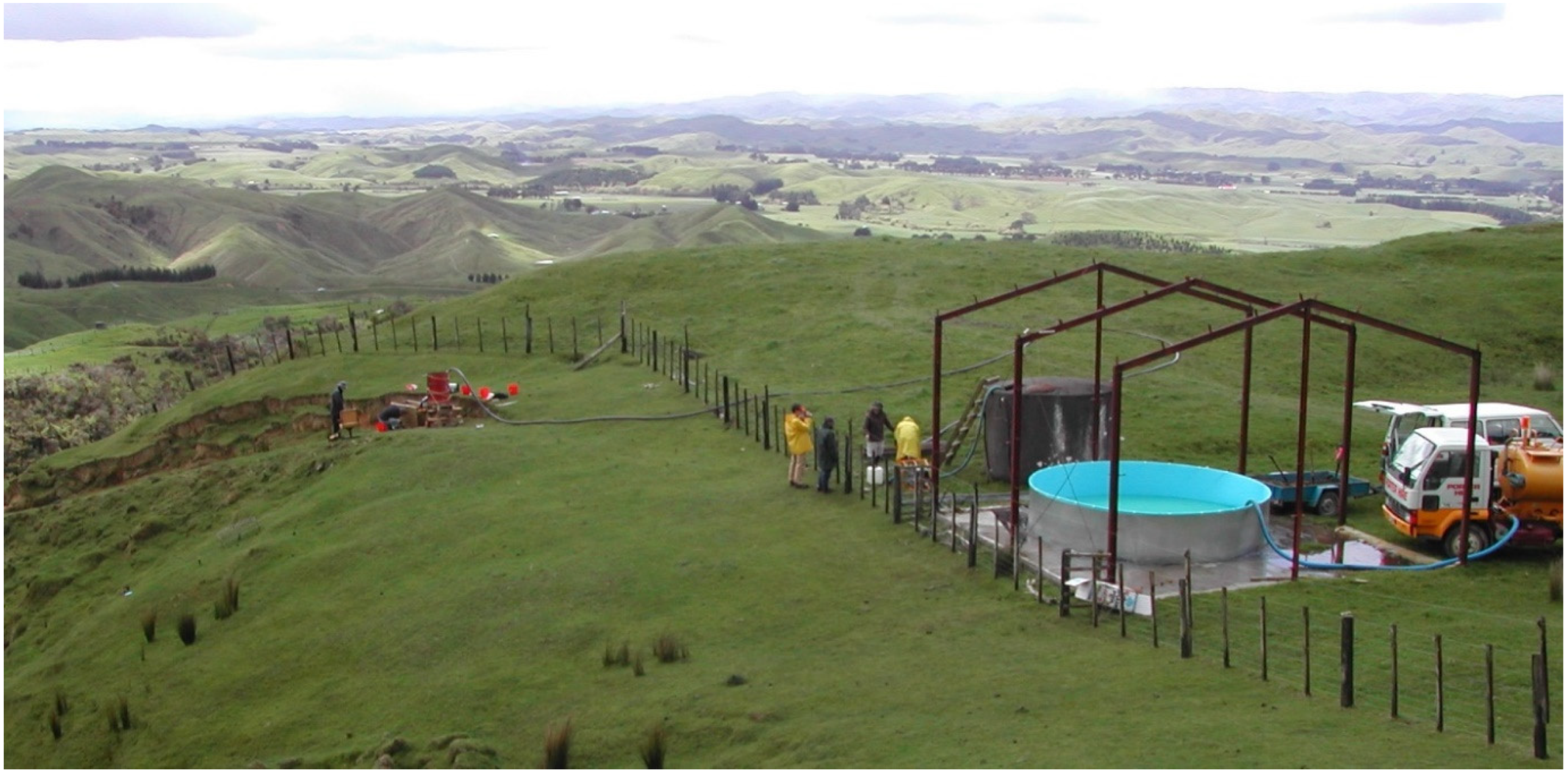
2.7. The Materials for Comparison of Calculations with Measurements

The calculations with any model must be compared with the measurements for possible validation and calibration. Field experiments were performed in the low-altitude hills of Ballantrae Hill Country Research Station near Woodville, New Zealand (Figure 2). The local soil belongs to Pallic Soils of the Wainui series formed on loess [26]. The entire depth of the A + AB-horizon is 40–50 cm. The organic carbon content in the topsoil is 2.4%, and 0.4% in the parent loess. The topsoil is well-structured and highly water-stable: wet sieving of 2–4 mm aggregates for 30 min showed that 88% was retained for this class. The aggregate stability in the parent loess is much lower—the proportion of aggregates retained on the sieve was 7.6%. The mean size of soil aggregates obtained by dry sieving D_s ≈ $\sqrt{\frac{4S_a}{\pi }}$ was 1.83 mm, with a standard deviation σ_D = 0.88 mm. The aggregates were flattened, to a plate or ellipsoidal shape, with $\frac{D_m}{D_s}$ ≈ 1/3. The mean soil strength, measured with a tor-vane, was nearly equal for parent loess and topsoil: 52 and 51 kPa, respectively. The soil density ρ_s was 1460 and 1230 kg/m³, respectively.

Two erosion plots were organized on two steep slopes (at straight parts), which accurately represent the gully beds. The abandoned road on the parent loess was used to organize plot 1, at 17.4 m long and 0.55 m wide with an inclination of 0.235 (13.2°). Plot 2 was cut into the topsoil by the removal of the upper 5–7 cm of soil with grass cover to avoid grass roots’ influence on the erosion rate. The residual content of thin roots in the soil was less than 0.1% by weight (the initial content in the upper 5–7 cm was about 4%). Plot 2 was 11.5 m long, 0.32 cm wide and had an inclination of 0.483 (25.8°).

Experiments were conducted during November 2001. Five runs, each lasting half an hour, were performed at each plot with discharges of 1.48–11.2 L/s controlled with a V-notch weir (

Table 1. The main characteristics of the experiments in Ballantrae Hill Country.

N Plot–Soil–Run	Q, l/s	U, m/s	W, m	d, m	U*	σU	E, m/s	Re	Fr
1–b2–3	3.13	1.19	0.46	0.0057	0.12	0.26	2.29 × 10−7	6020	5.0
1–b2–4	4.01	1.30	0.46	0.0067	0.13	0.28	2.33 × 10−7	7670	5.1
1–b2–5	5.12	1.40	0.47	0.0077	0.14	0.30	2.29 × 10−7	9510	5.1
1–b2–6	6.86	1.53	0.49	0.0092	0.15	0.33	5.49 × 10−7	12,340	5.1
1–b2–7	11.13	1.79	0.51	0.0121	0.17	0.38	1.66 × 10−6	19,070	5.2
2–b4–3	1.48	1.20	0.28	0.0043	0.14	0.31	3.13 × 10−8	4590	5.8
2–b4–4	2.22	1.56	0.29	0.0049	0.15	0.33	4.8 × 10−8	6750	7.1
2–b4–5	3.04	1.66	0.29	0.0062	0.17	0.38	8.54 × 10−8	9100	6.7
2–b4–6	4.01	1.91	0.30	0.0070	0.18	0.40	1.4 × 10−7	11,810	7.3
2–b4–7	5.92	2.15	0.31	0.0089	0.21	0.46	3.49 × 10−7	16,830	7.3

Key: Q—discharge, U—mean velocity, W—flow width, d—flow depth, U_*—kinematic velocity, σ_U—velocity fluctuation standard deviation (from Equation (19)), E—erosion rate, Re—Reynolds number, Fr—Froude number.

). Flow width was measured at 8–10 cross-sections and the mean flow velocity was measured using salt injections. The mean flow depth was calculated from discharge, flow width and velocity. All flows were turbulent and supercritical. Samples of water with sediment particles, with a total volume of about 4 L, were taken at the end of the plot and at the end of the half-an-hour run. The sediment concentration was estimated by means of the standard procedure of filtering, drying, weighting and dividing based on water volume.

The coefficient k_U for ellipsoidal aggregates is $\frac{3\rho }{16{\rho }_s}\left(0.1+0.42\frac{S_d}{S_a}\right)$ and varied in the range 0.026–0.04 for the first plot and 0.031–0.047 for the second (depending on S_a/S_d ratio in the range 2–4). The standard deviation of velocity fluctuations was ${\sigma }_U\cong 2.1U_{*}$ (according to [19]).

The coefficient k_D = $\cos \mathsf{\gamma }\frac{g\left({\rho }_s-\rho \right)}{2{\rho }_s}\sin \left[\arctan \left(0.238\frac{S_a}{S_d}\right)\right]$ was in the range 0.44–0.64 for the first plot and 0.24–0.35 for the second.

The coefficient k_C = $D\frac{S_b}{2{\rho }_s{V}_a}=\frac{3}{8{\rho }_s}\frac{S_b}{S_a}\approx \frac{3\left(1-{\epsilon }_{}^{2/3}\right)}{8{\rho }_s}$ was 2.04 × 10⁻⁴ for the first plot and 1.54 × 10⁻⁴ for the second. The variation coefficient for cohesion was estimated as 0.59 in the experiments with the cutting of the surface of the soil sample with a moving blade [24].

The relationship between the erosion rate and the flow velocity shows a higher erosion rate at plot 1 than at plot 2 for the same velocity (Figure 3). This is explained by the higher soil aggregate stability and organic matter content in the soil at plot 2. The power–law functions describe these relationships well. The exponents are different for these two plots (5.2 for the first and 4.1 for the second) and differ from the function commonly used in the majority of shear–stress erosion models (see, for example, [27]).

3. Results

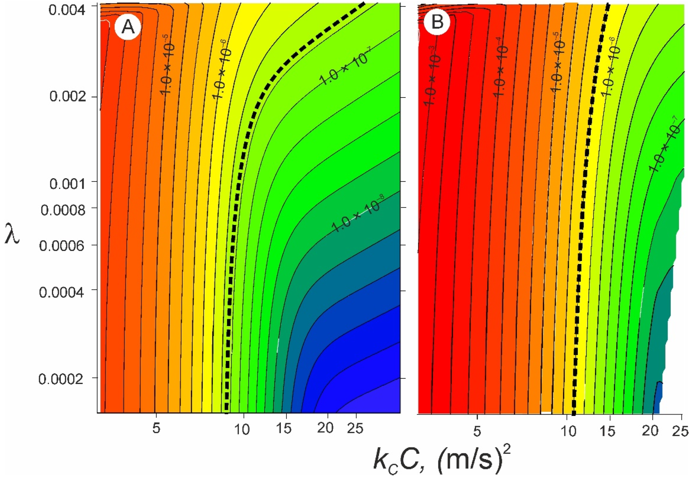
3.1. General Numerical Experiments

The first set of calculations with the algorithm described above (Figure 1) show the erosion rate change through time (Figure 4). In the numerical experiments for different flow velocities, soil was “eroded” for 1800 or 3600 s. During this period, the mean cohesion of the soil surface layer and the instant erosion rate changed through time due to the action of soil armoring and soil loosening. The temporal trend changed its sign depending on the sign of the cumulative effect of armoring and loosening. The most common scenario was a general decrease in soil mean cohesion during the first 500 s, then a slight increase and stabilization after about 1000 s in the experiment. The erosion rate decreased during the first 5–20 s, then significantly increased and stabilized after about 1000 s in the experiment. The temporal changes in the percentage of the area of erodible soil P_E, where the driving forces were greater than the resistance forces, corresponded with the trends in erosion rate. The influence of the soil particle size on the erosion rate was much smaller than that of cohesion, and is thus not discussed further.

The temporal trends in the mean cohesion of the surface layer and in the erosion rate are controlled by changes in cohesion PDFs (Figure 5). A very small part of the PDF of the cohesion force at the segment, overlapping the PDF of the driving force (Figure 5A), controls the rate of erosion and the percentage of erodible soil surface P_E (Figure 4C). The values of probability density (PD) are very small here (Figure 5B). Therefore, numerical experiments focusing on this segment require precise calculations.

The PD at the segment around the mode of PDF increases through time and the mode position shifts to lower values of cohesion due to the loosening of soil at the surface (Figure 5C). The PD at the main part of PDF to the right of the mode mostly decreases until ~500 s, and then stabilizes (Figure 5D). The part of the PDF with a soil cohesion force greater than the driving force controls the temporal changes in the mean cohesion of the soil surface layer.

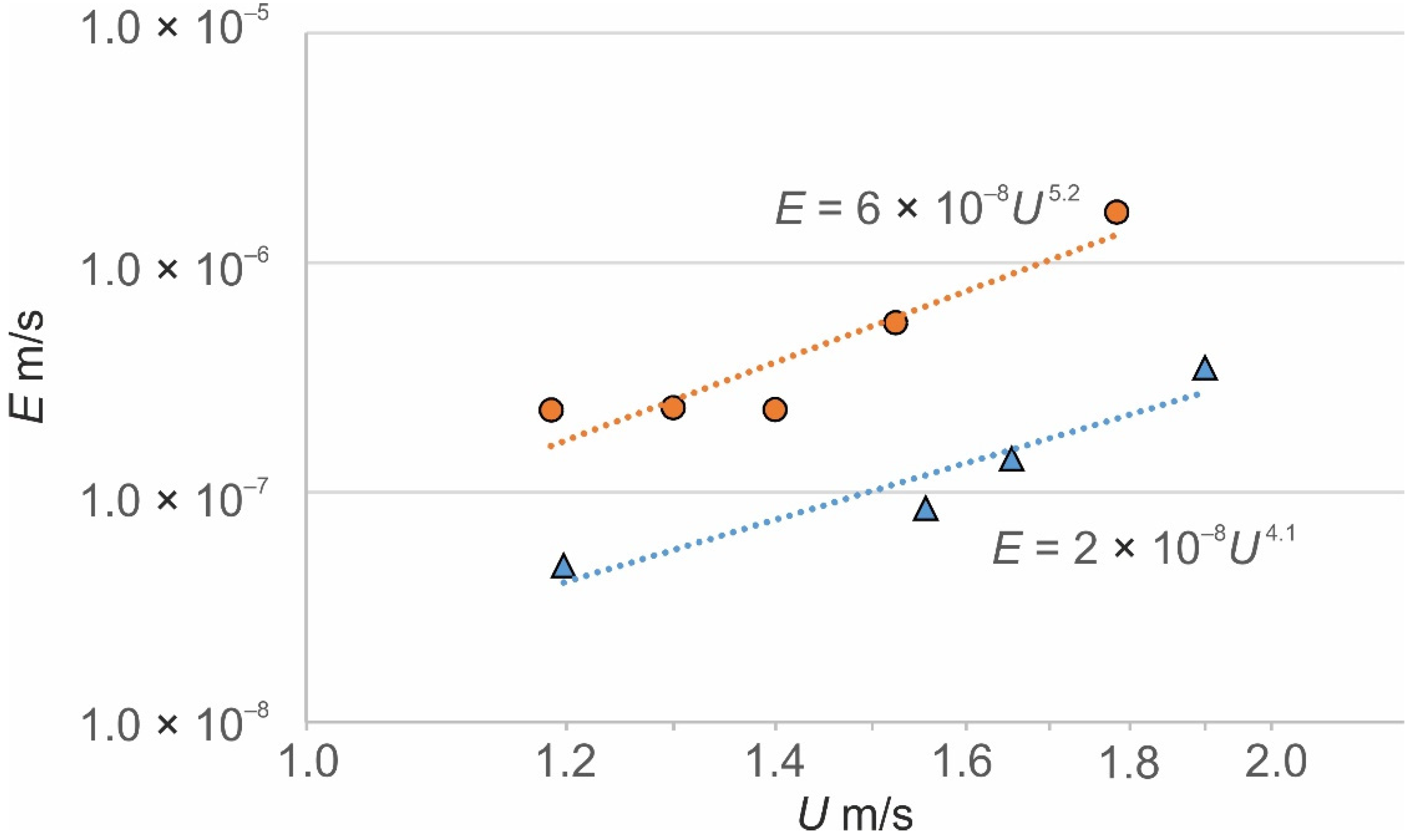
3.2. The Comparison of Calculated Erosion Rates with the Measured

In the situation where one of the main factors of erosion, i.e., the resisting forces of soil cohesion, are indefinite, it is possible to find these indefinite characteristics by comparing the measured rates of erosion and calculating them with Equations (17)–(28).

Numerical experiments were performed with input characteristics from Table 1. The fields of erosion rate E at given flow velocities were calculated for a variety of initial soil cohesions k_CC and parameters λ in the failure function. Examples of such fields, represented by isolines of erosion rate E, are shown in Figure 6 for two runs in plot 1. The soil erosion rate is characterized by equifinality. The calculation for each pair of k_CC and λ at a given flow velocity leads to a unique value of the resulting erosion rate E. At the same time, calculations for different pairs of initial soil cohesion and parameter λ at a given flow velocity lead to the same resulting erosion rate, forming the isoline in Figure 6. The same measured rate of erosion at a given flow velocity, shown by bold dashed isolines, can also appear with different combinations of soil properties. This set of numerical experiments shows that the result of a single run with measured characteristics of flow and erosion rate cannot be used to find indefinite soil properties (initial soil cohesions k_CC and parameters λ), which are used in the proposed model.

The shape of the erosion rate isolines is different for different flow velocities. Therefore, a combination of such isolines can probably narrow the region of indefinite soil properties.

Keeping the initial soil cohesion constant in the numerical experiments for a given flow velocity, it is possible to minimize the difference between measured erosion rates and calculated ones with Equations (24)–(28) by varying parameter λ. The points in Figure 7 and Figure 8 shows the optimal erosion rates for each flow velocity from the measurements at Ballantrae Hill Country for different combinations of k_CC and λ. The intersections of erosion rate isolines narrow the range of such combinations for the set of experiments on the same soil with different flow velocities (green borders at Figure 7 and Figure 8). The soil at plot 1 is characterized by a cohesion force k_CC in the range of 12–14 m²/s² (or C = 60–70 kPa), a parameter λ in the range of 0.0025–0.004 and the percentage of the area, occupied by erodible soils after 3600 s of the armoring–loosening cycles, in the range of 0.55–0.7%.

The same types of calculations were performed for the flow velocities and erosion rates, measured at plot 2 (Figure 8). They show that the soil is characterized (see green boarders) by an initial cohesion force k_CC in the range of 27–31 m²/s² (or C = 180–200 kPa), a parameter λ in the range of 0.0015–0.002, and the percentage of the area, occupied by erodible soils after 3600 s of the armoring–loosening cycles, in the range of 0.35–0.55% per second.

These results are in general accordance with the measured characteristics at these two plots. The cohesion, measured with a tore—vane, was about 50 kPa at both plots, which is rather close to the estimates provided by modelling for plot 1. The much higher estimate for the cohesion for plot 2 is explained by the anti—erosion effect of the organic matter in the soil (2.4%). The parameter λ in the failure function, with controls the rate of soil loosening during erosion and the rate of increase in the area of eroded soil, which controls the rate of erosion, are both two—fold larger at plot 2 than at plot 1. This is also due to the anti—erosion effect of organic matter. These observations show that erosion at plot 1 was due to the destruction of within—aggregate links, and so small soil particles were moved from the soil surface. The erosion at plot 2 was due to the destruction of between—aggregate links, and so rather large particles were collected at the end of the plot (Figure 9). This difference in the erodibility of the soil at plots 1 and 2 is also well—illustrated by the aggregate stability tests: wet sieving aggregates for 30 min showed that 88% was retained for soil from plot 2 and only 7.6% was retained for soil from plot 1.

The numerical experiments (Figure 7 and Figure 8) show the possibility to estimate the main soil characteristics used in the model through gully erosion simulation in flume or direct measurements of the gully erosion rate in the field with a variety of flow velocities on the same soil. The number of such experiments is limited now, and there is a large field for future investigations.

4. Discussion

The combination of classical deterministic mechanics—Newton’s second law—and the stochastic description of the erosion control factors (driving and resistance forces) has led to the development of the stochastic gully erosion model (STOGEM).

The mean erosion rate is calculated with the algorithm in Figure 1 using the equation of the force balance acting on a soil particle in a water flow with the PDFs of flow velocity, soil aggregate size and cohesion, including several model parameters, such as k_U, k_D and k_C. The mathematical methods for the calculation of the PDF of the function of stochastic variables, knowing the PDFs of these stochastic variables [14], are used. The relationships between the main factors of erosion (for example, flow velocity) and erosion rate are theoretically determined within the model for a given combination of input data. This theory opens up a new way for better understanding the experimental results of soil erosion, and demonstrates the direction for future investigations. It is possible to estimate the main soil characteristics used in the model by gully erosion simulation in flume or direct measurements of the gully erosion rate in the field with a variety of flow velocities in the same soil. The results of numerical experiments are consistent with the measurements in the laboratory flumes [15] and show the same stages of erosion development in cohesive soils.

The relationships between the rate of erosion and control factors are not pre—installed in this model. This is the main advantage and its main difference from empirical USLE—type [28] and “process—based” shear stress—type models [27]. STOGEM also contains novel elements compared to previously published stochastic models of soil erosion [29,30,31,32].

The expression for cohesive soil erosion rate calculation (Equation (17)) can be naturally included into the equation of deformation in models such as GULTEM or DYNGUL [10], or any other process—based model of gully erosion instead of using empirical shear—stress type formulas.

The theoretical approach to gully erosion calculations is far from achieving direct application in soil conservation practice. There are many unknown processes and parameters, mostly related to changeable and complicated matters, such as the soil. The list of possible improvements and clarifications of the model is long. It is obvious that most of the parameters taken as constants in the above—described model (soil particle shape, porosity, etc.) are stochastic variables. The exponential failure function is the simplest option to model the process of soil loosening, and the wet—sieving test of aggregate stability shows that the Weibull function better explains this process. The different resistance to erosion of the links within and between soil aggregates must be investigated. The effect of raindrops on erosion by water in the gullies must also be taken into account.

The general limitation of this model is the requirement of erosion of the surface layer particle by particle. This requirement may not be respected at high rates of soil loosening and high velocities. The processes of transport and the deposition of eroded soil particles are not taken into account, and the influence of such processes can be important [33]. The further comparison of the measured rates of gully erosion performed in the frame of this model with calculated ones will reveal other details necessary for stochastic modelling.

5. Conclusions

The stochastic gully erosion model (STOGEM) is based on a combination of deterministic mechanics—Newton’s second law—and the stochastic description of the erosion control factors. The main proposition in this model is that the depth of the active surface layer of eroded cohesive soil is equal to one particle diameter, and erosion develops particle by particle. The processes of transport and deposition of eroded soil particles are not taken into account. The erosion rate at the gully bed is calculated directly from the equation of the balance between the driving and resistance forces acting on a soil particle in flowing water. All factors of erosion—flow velocity, soil aggregate size and cohesion—are regarded as stochastic variables, described by probability density functions. The probability density function of cohesion in the model varies through time and space during an erosion event due to the changes in soil composition, namely armoring and loosening. This theory is still far from achieving practical application, but opens up a new way for better understanding the experimental results of gully erosion and demonstrates the direction for future investigations.

References

1. Ireland, H.A.; Eargle, D.H.; Sharpe, C.F.S. Principles of Gully Erosion in the Piedmont of South Carolina; Technical Bulletins 167374; U.S. Department of Agriculture, Economic Research Service: Washington, DC, USA, 1939. [Google Scholar]
2. Watson, D.A.; Laflen, J.M.; Franti, T.G. Estimating Ephemeral Gully Erosion; Paper No. 86-2020; American Society of Agricultural Engineers: St. Joseph, MI, USA, 1986; pp. 1–16. [Google Scholar]
3. Kosov, B.F.; Nikolskaya, I.I.; Zorina, Y.F. Experimental research of gullies formation. Exp. Geomorphol. 1978, 3, 113–140. (In Russian) [Google Scholar]
4. Sidorchuk, A.Y.; Golosov, V.N. Erosion and sedimentation on the Russian Plain, II: The history of erosion and sedimentation during the period of intensive agriculture. Hydrol. Process. 2003, 17, 3347–3358. [Google Scholar] [CrossRef]
5. Montgomery, D.R. Erosional processes at an abrupt channel head: Implications for channel entrenchment and discontinuous gully formation. In Incised River Channels; Darby, S., Simon, A., Eds.; Wiley: New York, NY, USA, 1999; pp. 247–276. [Google Scholar]
6. Panin, A.; Borisova, O.; Konstantinov, E.; Belyaev, Y.; Eremenko, E.; Zakharov, A.; Sidorchuk, A. The Late Quaternary evolution of the upper reaches of fluvial systems in the southern East European Plain. Quaternary 2020, 3, 31. [Google Scholar] [CrossRef]
7. Poesen, J.W.A.; Torri, D.; Vanwalleghem, T. Gully erosion: Procedures to adopt when modelling soil erosion in landscapes affected by gullying. In Handbook of Erosion Modelling; Morgan, R.P.C., Nearing, M.A., Eds.; Wiley—Blackwell: Chichester, UK, 2011; pp. 360–386. [Google Scholar] [CrossRef]
8. Torri, D.; Poesen, J. A review of topographic threshold conditions for gully head development in different environments. Earth Sci. Rev. 2014, 130, 73–85. [Google Scholar] [CrossRef]
9. Rose, C.W.; Yu, B.; Ward, D.P.; Saxton, N.E.; Olley, J.M.; Tews, E.K. The erosive growth of hillside gullies. Earth Surf. Process. Landf. 2014, 39, 1989–2001. [Google Scholar] [CrossRef]
10. Sidorchuk, A. Models of gully erosion by water. Water 2021, 13, 3293. [Google Scholar] [CrossRef]
11. Sidorchuk, A.; Smith, A.; Nikora, V. Probability distribution function approach in stochastic modelling of soil erosion. IAHS Publ. 2004, 288, 345–353. [Google Scholar]
12. Du Boys, P. Le Rhône et les Rivières a Lit affouillable. Ann. Ponts Chaussées 1879, 18, 171–195. (In French) [Google Scholar]
13. Sidorchuk, A. Stochastic modelling of erosion and deposition in cohesive soils. Hydrol. Process. 2005, 19, 1399–1417. [Google Scholar] [CrossRef]
14. Ventsel, E.S. The Probability Theory, 4th ed.; (Teoriya Veroyatnostey); Nauka: Moscow, Russia, 1969; p. 564. (In Russian) [Google Scholar]
15. Mirtskhulava, T.E. Principles of Physics and Mechanics of Channel Erosion (Osnovy Fiziki i Mekhaniki Erozii Rusel); Gidrometeoizdat: Leningrad, Russia, 1988; p. 303. (In Russian) [Google Scholar]
16. Lamb, M.P.; Dietrich, W.E.; Venditti, J.G. Is the critical Shields stress for incipient sediment motion dependent on channel—bed slope? J. Geophys. Res. 2008, 113, F02008. [Google Scholar] [CrossRef] [Green Version]
17. Su, Z.A.; Xiong, D.H.; Dong, Y.F.; Zhang, B.J.; Zhang, S.; Zheng, X.Y.; Fang, H.D. Hydraulic properties of concentrated flow of a bank gully in the dry-hot valley region of southwest China. Earth Surf. Process. Landf. 2015, 40, 1351–1363. [Google Scholar] [CrossRef]
18. Nikora, V.I.; Goring, D.G. ADV measurements of turbulence: Can we improve their interpretation? J. Hydraul. Eng. 1998, 124, 630–634. [Google Scholar] [CrossRef]
19. Nezu, I.; Nakagawa, H. Turbulence in Open Channel Flows (IAHR Monograph); Balkema: Rotterdam, The Netherlands, 1993; p. 286. [Google Scholar]
20. Gardner, W.R. Representation of soil aggregate—Size distribution by a logarithmic—Normal distribution. Soil Sci. Soc. Am. Proc. 1956, 20, 151–153. [Google Scholar] [CrossRef]
21. Perfect, E.; Kay, B.D.; Ferguson, J.A.; da Silva, A.P.; Denholm, K.A. Comparison of functions for characterizing the dry aggregate size distribution of tilled soil. Soil Tillage Res. 1993, 28, 123–139. [Google Scholar] [CrossRef]
22. Elliot, W.J.; Liebenow, A.M.; Laflen, J.M.; Kohl, K.D. A Compendium of Soil Erodibility Data from WEPP Cropland Soil Field ERODIBILITY Experiments 1987 and 1988; (NSERL Report No. 3); The Ohio State University: Columbus, OH, USA; USDA Agriculture Research Service: Washington, DC, USA, 1989; p. 317. [Google Scholar]
23. Barral, M.T.; Arias, M.; Guerif, J. Effects of iron and organic matter on the porosity and structural stability of soil aggregates. Soil Tillage Res. 1998, 46, 261–272. [Google Scholar] [CrossRef]
24. Sidorchuk, A.; Nikora, V.; Marsden Fund Project “Stochastic Mechanics of Soil Erosion”. LCR203 Final Report Summary. 2005. Available online: http://fluvial-systems.net/Marsden%20Fund%20award/MarsdenFundReport.html (accessed on 9 January 2022).
25. Billinton, R.; Allan, R.N. System reliability evaluation using probability distributions. In Reliability Evaluation of Engineering Systems; Springer: Boston, MA, USA, 1992; Chapter 7; pp. 221–259. [Google Scholar]
26. Hewitt, A.E. New Zealand Soil Classification; Landcare Res. Sci. Series 1; Manaaki Whenua Press: Lincoln, New Zealand, 1998; p. 124. [Google Scholar]
27. Foster, G.R.; Lane, L.J.; Nearing, M.A.; Finkner, S.C.; Flanagan, D.C. Erosion component. In USDA Water Erosion Prediction Project: Hillslope Profile Model Documentation; NSERL Report No. 2; Lane, L.J., Nearing, M.A., Eds.; National Soil Erosion Research Laboratory, USDA—ARS: Lafayette, IN, USA, 1989; Chapter 10. [Google Scholar]
28. Renard, K.G.; Foster, G.R.; Weesies, G.A.; McCool, D.K.; Yoder, D.C. Predicting Soil Erosion by Water: A Guide to Conservation Planning with the Revised Universal Soil Loss Equation (RUSLE). In Agriculture Handbook 703; U.S. Dept. Agriculture: Washington, DC, USA, 1997. [Google Scholar]
29. Partheniades, E. Erosion and deposition of cohesive soils. J. Hydraul. Div. Am. Soc. Civ. Eng. 1965, 91, 105–139. [Google Scholar] [CrossRef]
30. Nearing, M.A. A probabilistic model of soil detachment by shallow flow. Trans. Am. Soc. Agric. Eng. 1991, 34, 81–85. [Google Scholar] [CrossRef]
31. Wilson, B.N. Development of fundamentally based detachment model. Trans. Am. Soc. Agric. Eng. 1993, 36, 1105–1114. [Google Scholar] [CrossRef]
32. Winterwerp, J.C.; van Kesteren, W.G.M.; van Prooijen, B.; Jacobs, W. A conceptual framework for shear flow–induced erosion of soft cohesive sediment beds. J. Geophys. Res. 2012, 117, C10020. [Google Scholar] [CrossRef] [Green Version]
33. Hairsine, P.B.; Rose, C.W. Modeling water erosion due to overland flow using physical principles: 2. Rill flow. Water Resour. Res. 1992, 28, 245–250. [Google Scholar] [CrossRef]
Figure 1. Algorithm of the calculation of the gully erosion rate with the stochastic model. The explanation is given in the text.
Earth 03 00015 g001
Figure 2. Experimental site at the Ballantrae Hill Country Research Station near Woodville, New Zealand.
Earth 03 00015 g002
Figure 3. The relationship between flow velocity U and erosion rate E for plot 1 (circles) and plot 2 (triangles) in the experiments in Ballantrae Hill Country.
Earth 03 00015 g003
Figure 4. Change through time in calculated specific soil cohesion force kCC (A), erosion rate E (B) and the percentage of the area occupied by erodible soils after the armoring–loosening cycles PE,% (C) for different flow velocities. The initial k C is 17, the parameter of loosening λ = 0.001, and other parameters were obtained from plot 2.
Earth 03 00015 g004
Figure 5. Temporal changes in the PDF of soil cohesion for a flow velocity of 2.15 m/s. (A) PDF of driving force (green line) and PDFs of cohesion force, initial (red line) and at the stage of rapid changes (black lines). Two modes show two stage of stabilization. (B) Temporal changes in probability density of cohesion force for kCC = 4 m2/s2 at the segment, overlapping with the PDF of driving forces. (C,D) Changes in the probability density of cohesion force for kCC = 15–20 and 30 m2/s2. Numerical experiments for initial k C C = 30, parameter of loosening λ = 0.0015, and other parameters obtained from plot 2.
Earth 03 00015 g005
Figure 6. The fields in isolines of erosion rate E (m/s), calculated for varying initial cohesion k C C and the parameter of loosening λ for two flow velocities from plot 1: (A) 1.4 m/s and (B) 1.79 m/s. The measured rate of erosion at a given flow velocity is shown by a bold dashed isoline.
Earth 03 00015 g006
Figure 7. The possible combinations of initial specific soil cohesion force (kCC, m2/s2) with parameter λ in the failure function, which lead to the same resulting erosion rate at a given flow velocity (A), and of the percentage of the area, occupied by erodible soils after 3600 s of the armoring–loosening cycles PE,% (B). The green box shows the possible range of soil properties, which fits the measured flow velocity and erosion rate in plot 1.
Earth 03 00015 g007
Figure 8. The possible combinations of initial specific soil cohesion force (kCC, m2/s2) with parameter λ in the failure function, which lead to the same resulting erosion rate at a given flow velocity (A), and of the percentage of the area, occupied by erodible soils after 3600 s of the armoring–loosening cycles PE,% (B). The green box shows the possible range of soil properties, which fits the measured flow velocity and erosion rate in plot 2.
Earth 03 00015 g008
Figure 9. Soil aggregates and particles, collected at the end of plot 2 during the run 2–b4–3.
Earth 03 00015 g009