Analysis of Expected Climate Extreme Variability with Regional Climate Simulations over Napoli Capodichino Airport: A Contribution to a Climate Risk Assessment Framework

Abstract

In recent years, the scientific community has paid particular attention to the analysis of extreme events, such as heat waves, droughts, and intense rain events that have caused loss of human life and significant economic damage. Climate-related extremes generally produce large impact on infrastructures, especially on those with insufficient design, while some infrastructures may become inadequate under the effects of severe extremes. In the particular case of airports, the increase in frequency and severity of extreme weather events will worsen their deterioration rate. This work presents an analysis of the expected climate variability over Napoli Capodichino Airport, using climate projections generated by the Regional Climate Model COSMO-CLM. Simulations were performed over Italy, employing a spatial resolution of approximately 8 km. The time period simulated was 1979–2100, and, in particular, the CMIP5 historical experiment (based on historical greenhouse gas concentrations) was used for the period 1979–2005, while, for the period 2006–2100, two different simulations were performed, employing the Representative Concentration Pathways IPCC RCP4.5 and RCP8.5 greenhouse gas concentrations. The meteorological situations over the airport have been analyzed, along with the identification of conditions that could cause relevant impact on airport environment. In particular, extreme summer temperatures may exceed design standards, leading to heat damage to surfaces, while runways or aprons may have trouble due to the surface melting during peak heat periods. Long term changes in the directions of wind can adversely affect the usability of runways, while changes in wind shear could modify strength and frequency of clear-air turbulence. Analyses have been performed considering suitable Extreme Events Indicators (EWI), both on past trends and on numerical projections over future periods, with the aim of contributing to the definition of a risk assessment methodology based on the combination of the frequency and of the severity of meteorological hazards.

1. Introduction

Climate change is one of the biggest challenges facing society in the 21st century. Climate modifications can have negative impacts on ecosystems, economy, health, agriculture production, and water and food availability [1]. Different studies conducted on global and local scales agree that there will be a decrease in rainfall and a growing trend in minimum and maximum temperatures [2]. In recent years, the scientific community has paid particular attention to the analysis of extreme events such as heat waves, droughts, and intense rain events that have caused loss of human life and significant economic damage [3]. In fact, extreme weather events have a strong impact at global level, and their increase in terms of frequency and severity is due to climate change [4]. The Sixth Assessment Report of IPCC (AR6) [5] clearly states that the evidence of observed changes in extremes and their attribution to human activities has strengthened since the previous AR5, and that many changes in the climate system will become larger in close relation to the increasing global warming.

Climate-related extremes generally produce large impact on infrastructures, especially on those with insufficient design, while some infrastructures may become inadequate under the effects of severe extremes. Critical infrastructures include transportation systems, urban buildings, water systems, and communication systems, and in general those which provide fundamental functions to sustain the society; a breakdown of them could lead to significant economic losses and high numbers of human deaths [6].

Transport infrastructures play a major socio-economic role, and particular airports, as global connectors, are crucial for the world economy and the transportation system. Even if they are designed to cope with various stresses during their life, the intensification of frequency and severity of extreme weather events will increase their deterioration rate [7]. Indeed, according to a study by Eurocontrol (2013) focusing on Europe, 70% of airport delay is the result of severe weather events. Impacts over European airports differ according to their geographical position, climate zone, and local circumstances, but risks are larger in those areas where an increase in air traffic is expected, such as southern central Europe [8]. The traffic levels will increase by at least 50% in 2050, compared to 2000–2016 [9], therefore airports will have to face an increased challenge: managing intense meteorological events and a significant increase in air traffic.

Aviation in general is affected by changes in precipitation, temperature, sea-level rise, and wind [10]; moreover recent publications indicate that there are some additional potential impacts that may affect Europe’s aviation, along with other areas of the world, namely desertification and change in biodiversity. In southern Europe, the water shortage may cause soil erosion around the runway and sand damage to engines. Climate change may lead to changes in local biodiversity and wildlife migration patterns, and this could impact aircraft operation, particularly if there is an increase in heavy weight migratory bird populations in the area [9].

The importance of evaluating the impacts of climate changes over airports is widely recognized; however, the methodologies for quantifying the potential effects of climate change on aviation sector are still limited, especially in the Mediterranean area [11], although this region has been defined as a climate hot spot [12]. In recent years, a series of projects is being carried on in order to fill this gap. The VULCLIM Project (2016) by The French Technical Center for Civil Aviation (STAC) (2012) aimed to evaluate the vulnerability of French airports to climate change, identifying the climate variables with potential impacts on airports. In the frame of JRC PESETA III European Project (2018) [13], the analysis of the impacts of climate change on seaports, airports, and inland waterways was performed. Using spatial database and climate model outputs, this study has shown that many European airports located in coastal areas are at risk of inundation, due to sea level rise and sea storm surge, particularly on the North Sea coasts. The number of airports at risk of flooding is expected to increase by almost 60% between 2030 and 2080. In a study presented in the Environment Report of International Civil Aviation Organization [9], a risk analysis was conducted on the Istanbul Airport. The effects of four atmospheric parameters (precipitation, wind, temperature, and humidity/fog) on infrastructure and services were assessed using Regional Climate Models (RCMs) on the pillar years 2030, 2050, and 2080. Gratton et al. [11] assessed the impacts of climate change on ten Greek airports in terms of take-off performance of airliners, considering the headwind, surface conditions, temperature, and slope of the runway. They found that the take-off distance required for the medium-sized passenger jet Airbus A 320 increased by an average of 2.7 m/year, while for the smaller de Havilland DHC8-400, it was by 1.4 m/year. In a recent study, De Vivo et al. [14] proposed a methodology aimed to define the climate risk level on airports in the Mediterranean region.

According to [15], the first step needed to define a framework for risk assessment is to identify relevant climate change projections over the XXI century and their potential impacts on airport infrastructures. Projections could be obtained as result of simulations with Global Climate Models (GCMs), but their low spatial resolution does not allow their use on a local scale. For this reason, an appropriate downscaling of GCMs is required to produce climate projections on a specific area to a resolution between 1 and 50 km. The high spatial resolution allows a better representation of the climate in terms of average and extreme values, and to elaborate impact studies on both natural and anthropic systems, including infrastructures. Models are able to reproduce the climate system considering not only the natural forcing, but also the anthropogenic ones, which vary according with different scenarios. For example, Coffel et al. [16] used projections of daily temperatures from the CMIP5 model suite under the IPCC RCP 4.5 and RCP 8.5 scenarios to calculate future weight restrictions across a fleet of aircraft with different takeoff weights operating at a variety of airports.

Over Italy, a detailed analysis of the impacts of climate change in the aviation sector has not yet been conducted. In the present work, the expected climate extreme variability on the Capodichino airport, located in Naples has been analyzed. With approximately 10 million passengers in 2019 and approximately 10,000 tons of goods, it is a vital hub for the region’s economy. Climate projections considered in the present work were obtained with high resolution simulations performed over Italy with the RCM COSMO-CLM. Analyses have been performed considering suitable Extreme Events Indicators (EWI), both on past trends and on numerical projections over future periods, with the aim of contributing to the definition of a risk assessment methodology based on the combination of the frequency and of the severity of meteorological hazards with relevant impact on airports. With regards to extreme events, the Fifth IPCC Assessment Report [5] defines an extreme climatic event as one that is rare within its statistical reference distribution at a particular place and time. Generally, an extreme weather event would normally be as rare as or rarer than the 10th or 90th percentile of the observed Probability Density Function. Such events can be classified not only in terms of “rarity”, but also considering “severity” and “rapidity”, with respect to impact (severe or not severe) and longevity (acute or chronic) [17]. Severity in particular is a criterion used in climate science to define as “extreme” those events that cause large socio-economic losses.

The paper is organized as follows: in Section 2 the impact of extreme weather events on the airport is analyzed. Section 3 presents data and methods used, Section 4 summarizes the main results achieved, while in Section 5, the conclusion and the future works are discussed.

2. Impact of Extreme Weather on the Capodichino Airport

The geographical area considered in the present work (located in Southern Italy (Figure 1) includes the Napoli Capodichino airport (ICAO Code: LIRN) (40°53′ N, 14°17′ E). This area has a mild climate due to the proximity to the sea, but is also influenced by a colder internal zone characterized by the presence of mountains. High precipitation values are generally recorded along the coasts, generally up to 1000 mm/year, since most of the region is exposed to the humid westerly winds. Extreme meteorological events frequently affect this thunderstorm sensitive area, especially related to very intense precipitation and strong winds. They are likely associated with the increased Mediterranean temperature, in particular from the Tyrrhenian Sea, where storm cells are generated [18].

Even if the frequency and severity of extreme weather events over this area has been moderate during the 20th century as compared with other parts of Europe, in recent years these phenomena have caused considerable damage and widespread inconvenience. According with the Annual report of the Italian Association Legambiente (www.legambiente.it, accessed on 9 November 2021), 29 extreme events have hit the Campania region since 2010, and in particular six tornados, six flooding events due to intense rainfall, six river flooding events, and one landslide. According with statistical values provided by the University of Naples (meteo.unina.it), over the last 30 years, 12 days with very intense precipitation (>80 mm/day) have been recorded, leading to serious disruptions and extensive damages to the infrastructures. From the report elaborated by the Italian Agency for flight security (ANSV, www.ansv.it, accessed on 9 November 2021), it results that in the period 2007–2017, 449 episodes of wind shear took place over the Capodichino airport, with peaks of 97 in 2017 and 67 in 2014.

Impacts over European airports differ according to the geographical position, but risks are larger on those areas where an increase of air traffic is expected, such as southern Europe. Climate extremes can hit the European aviation sector in many manners. Specific impacts for the airport of Naples can be summarized as follows.

Higher temperatures may cause physical impacts. For example, extreme summer temperatures may exceed design standards leading to heat damage to surfaces, while runways or aprons may experience trouble due to surface melting during peak heat periods [19]. Furthermore, temperature has effects on the maximum take-off weight, since it affects aircraft performance and may cause cargo restrictions [10,11]. Limiting cargo implies serious economic losses for the companies. It is estimated that a restriction of 4% on the load is equivalent to a reduction of 12–13 passengers [16]. In addition, high temperature increases take-off and landing distances, and causes technical problems to the radars for air traffic control.

Very cold temperatures could lead to a decrease in lift, and also icing phenomena. Moreover, intense snowfall could jeopardize the usability of the airstrips, as happened in the event of 26–27 February 2018, when adverse weather conditions with snowfall caused delay and flight cancellations at the airport.

Heavy precipitation events could require increased separation distances between aircraft, affecting the airport throughput [8]. The current aerodrome surface drainage capacity may be insufficient to deal with more frequent and intense precipitation events, leading to increased risk of runway, taxiway, and electrical infrastructures flooding [19], as in the case of the extreme rainfall of 1 September 2018, which caused flooding of runways, and many flights diverted to other airports.

Long-term changes in the directions of wind can unfavorably affect the usability of runways [20], since runways constructed along the locally prevailing wind direction may experience more crosswinds due to deviations from the prevailing direction. Furthermore, the North-Atlantic jet stream could be stronger due to climate changes, leading to an increase of the transatlantic flight times towards the west [21,22]. Change in wind shear could modify strength and frequency of clear-air turbulence (CAT) [23] with implications on journey times.

An increase in sea storms is likely to occur in the near future, and could result in a temporary reduction in airport capacity and increase delays [9] unless preventive measures are taken, such as the construction of sea defenses [20].

Low visibility conditions, measured through the Meteorological Optical Range (MOR) provided by a visibilimeter, may result in restrictions on both ground and airborne movements at the airport and can reduce capacity. Moreover, these conditions are difficult to predict through weather and climate models. For this reason, semi-empiric formulae are employed in order to calculate specific indicators, such as the Fog Stability Index (FSI) [24] developed by the US Air Weather Service, and the Stoelinga–Warner index [25], which is calculated as a function of rain, snow, cloud water, and cloud ice.

Risks act on different time horizons, since some are on day-by-day basis, and others are in the long-term. The scientific community generally introduces indicators to evaluate progress towards goals and objectives. As better described in the next section, specific indicators can be defined in order to build descriptive and quantitative links between extreme weather events and the parts of the transport system that are affected by them, including infrastructure, operations, and indirect impact to third parties.

A summary of the climate extremes for the area of Naples, along with related impact and consequences, is presented in

Table 1. A summary of relevant climate extremes, impacts, and related consequences for the area of Napoli Capodichino airport.

Climate Extreme	Impact	Consequences
Cold temperature (T < 0°)	Slipperiness (ice formation, form of precipitation: rain/sleet/snowfall) Occurrence of freezing drizzle	Hazard for aviation and road traffic. Premature deterioration of road and runway pavements
Snowfall (>1 cm/24 h)	Slipperiness, troubles. The shallow snow layer might melt and then form an icy layer (if the road is not salted), for example after sunset	Increased accident rate
Wind gust (>25 m/s)	Reduced ground speed, reduced landing rate, reduced lift	Prolonged electricity cuts, delays and cancellations in air traffic
High temperature (T > 35°)	Heat damage to surface	Surface melting
Heavy precipitation (>20 mm/day)	Water rises to street level from drains	Damaged roads. Separation distance between aircraft. Delays
Hail (diameter > 5 cm)	Route blocked, airport closed; loss of situational awareness	Delays, diversion, accident, incident, ground damage
Lightning	Route blocked, airport ground operation interrupted, loss of situation awareness	Delays, diversion, accident, incident, maintenance, ground damage
Low visibility (MOR < 5 km)	Separation between aircraft increased	Delays, flight cancelled, airport closed.
Turbulence, wind shear	Changes in altitude/attitude occur; variations in indicated air speed	Passenger discomfort; structural damages

.

3. Materials and Methods

The analysis of future impacts of climate change on aviation encounters problems, since many relevant phenomena take place on space and time scales lower than scales resolved by current climate models. This problem is more pronounced when Global Climate Models are used, so downscaling techniques and statistical post-processing are needed to derive statistically reliable results for small-scale phenomena. This applies especially to high-impact weather phenomena, such as convection and related effects, ranging from low-level wind shear to hail and lightning strikes, CAT, and mountain-wave turbulence, as well as turbulence near thunderstorm tops, icing, and low-level wind shear.

The climate projections analyzed in the present work were obtained with the RCM COSMO-CLM [26] over a domain including the whole Italian peninsula, in the configuration optimized at CMCC Foundation (Centro Euro-Mediterraneo sui Cambiamenti Climatici) [27]. This model is the climate version of the operational non-hydrostatic mesoscale weather forecast model COSMO-LM developed by the German Weather Service (DWD). Simulations were performed employing a spatial resolution of 0.0715° (approximately 8 km). Initial and boundary conditions were provided by the GCM CMCC-CM [28], whose atmospheric component (ECHAM5) has a horizontal resolution of approximately 85 km. The time period simulated was 1979–2100, and, in particular, the CMIP5 historical experiment (based on historical greenhouse gas concentrations) was used for the period 1979–2005, while for the period 2006–2100, two different simulations were performed, employing the Representative Concentration Pathways IPCC RCP4.5 and RCP8.5 greenhouse gas concentrations [29,30]. RCPs identify the value of the additional radiative forcing (due to the anthropic contribution), expressed in W/m² expected for 2100 (compared to 1750 data). They form a set of greenhouse gas concentration and emissions pathways up to 2100, designed to support research on impacts and potential policy responses to climate change. RCP4.5 has been chosen since it is a trajectory describing radiative forcing with a stabilization after 2100, matching to policies that approximate the mitigation efforts proposed by the governments at the Paris COP21. RCP8.5 has been chosen since it is frequently referred to as “business as usual”, suggesting that is a likely outcome if governments do not make concentrated efforts to cut greenhouse gas emissions.

Since many practical problems require the knowledge of the behavior of extreme values, the Expert Team on Climate Change Detection and Indices (ETCCDI) has defined a core set of descriptive indices of extremes [31], so that each country can calculate the indices in exactly the same way and their analyses will fit into a global picture. These Extreme Events Indicators (EWIs) highlight different characteristics of extremes, including frequency, amplitude, and persistence, and are widely used to assess future changes (e.g., [32]). Some indices involve calculation of the number of days in a year exceeding specific thresholds: percentile thresholds (related to sites) and absolute thresholds (suitable in order to monitor extreme events that affect human society and the natural environment). They should be carefully selected in order to provide useful information. Indicators may reflect physical phenomena, related impacts, and effects on people and the environment (injuries, deaths, and ecological damages). Of course, a proper choice of climate indices could be made in terms of specific hazards considered, in consultation with stakeholders and policy makers.

The ability of the simulations considered in the present work to reproduce extreme events over Italy was assessed in [33], and, in particular, the climatology of a subset of ETCCDI indices for precipitation and temperature, finding a level of accuracy dependent on the region, especially in complex topographical areas. On average, it was found that a high resolution (less than 10 km grid cell size) is needed in order to properly simulate extreme events, since high resolution improves the simulation of small scale and high variability events. Accordingly with the considerations discussed in Section 2, the indicators described in

Table 2. Selection of Extreme Weather Events indicators based on Temperature/Precipitation/Wind considered in the present work.

Label	Description	Units
TXx	Annual maximum value of daily—maximum temperature	°C
SU	Summer days—annual count of days when the daily Tmax is above 35°	days/year
90p-Tmax	90th percentile of daily Tmax	°C
SDII	Mean precipitation in wet days (prec > 1 mm/day)	mm/day
R20	Number of days with precipitation > 20 mm/day	days/year
Rx1day	Maximum of daily precipitation	mm/day
90p-Prec	90th percentile of daily precipitation considering only the wet days (>1 mm)	mm/day
FG	Daily wind speed	m/s

have been selected, being considered as relevant for the present study. Even if airports in other latitudes operate under much warmer environments, the airport of Naples was designed in order to deal with conditions typical of the Mediterranean area, so this airport could not be able to bear very high temperatures. This applies also for what concerns high and intense precipitation events: there are airports (e.g., Munich, Germany) that have infrastructures suitable to manage this condition, because they are used to working in very rainy environments. Intense snowfalls could have also relevant impact, since the Capodichino airport is not sufficiently equipped to manage this condition; however, snow metrics were not considered in the present analysis because, in Naples, the snow is infrequent (the annual number of days with snow rarely exceeds 5), and an RCM can hardly capture so rare events. Moreover, long series of data related to the snow are not available over Campania region.

Daily temperature, precipitation and wind data from the weather station at Napoli Capodichino airport were considered in order to validate the model. These data were provided by the SCIA (Sistema nazionale per l’elaborazione e diffusione di dati climatici) system (National system for the collection, elaboration, and diffusion of climate data) developed by ISPRA (Istituto Superiore Protezione e Ricerca Ambientale) [34] (www.scia.isprambiente.it, accessed on 9 November 2021).

4. Results

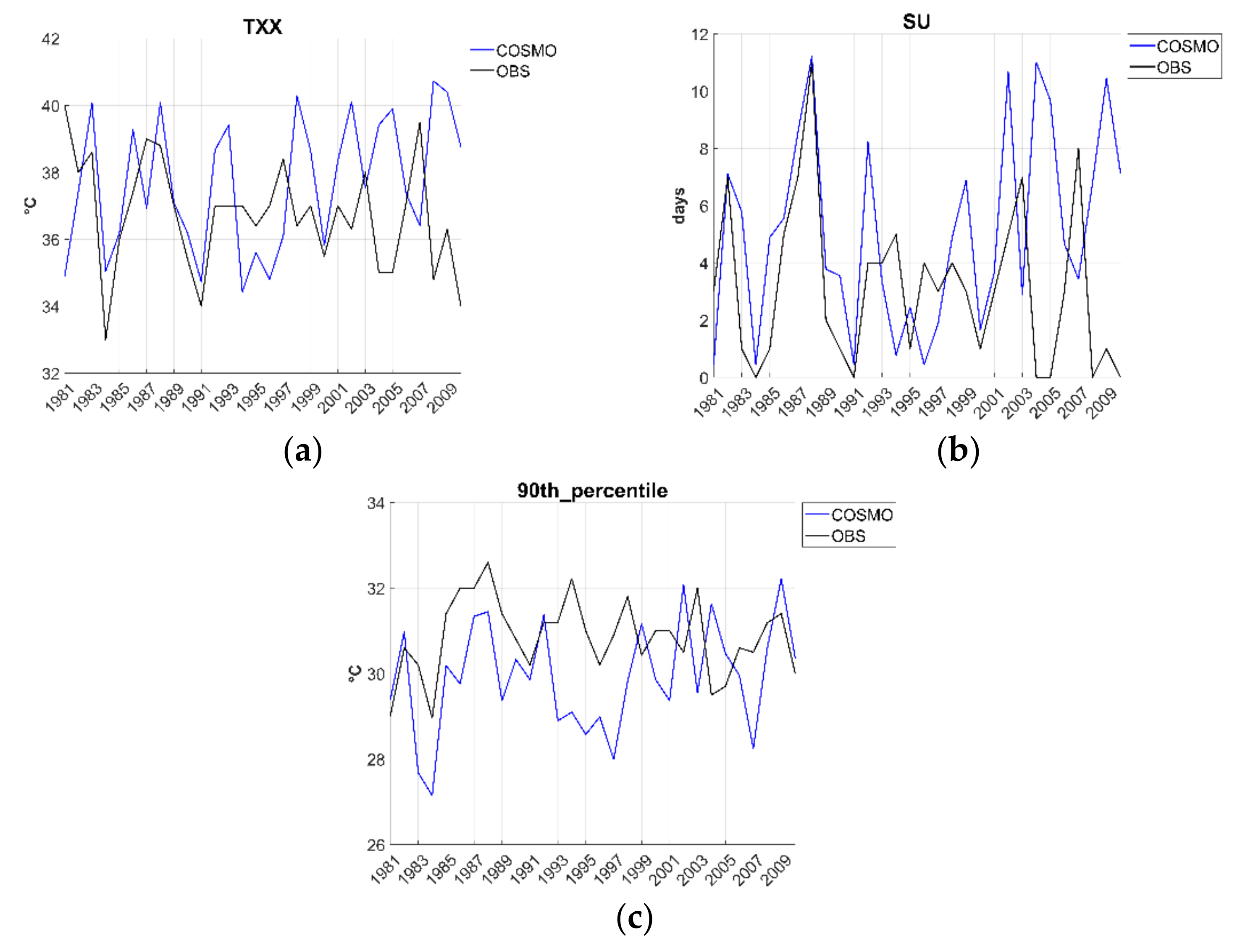
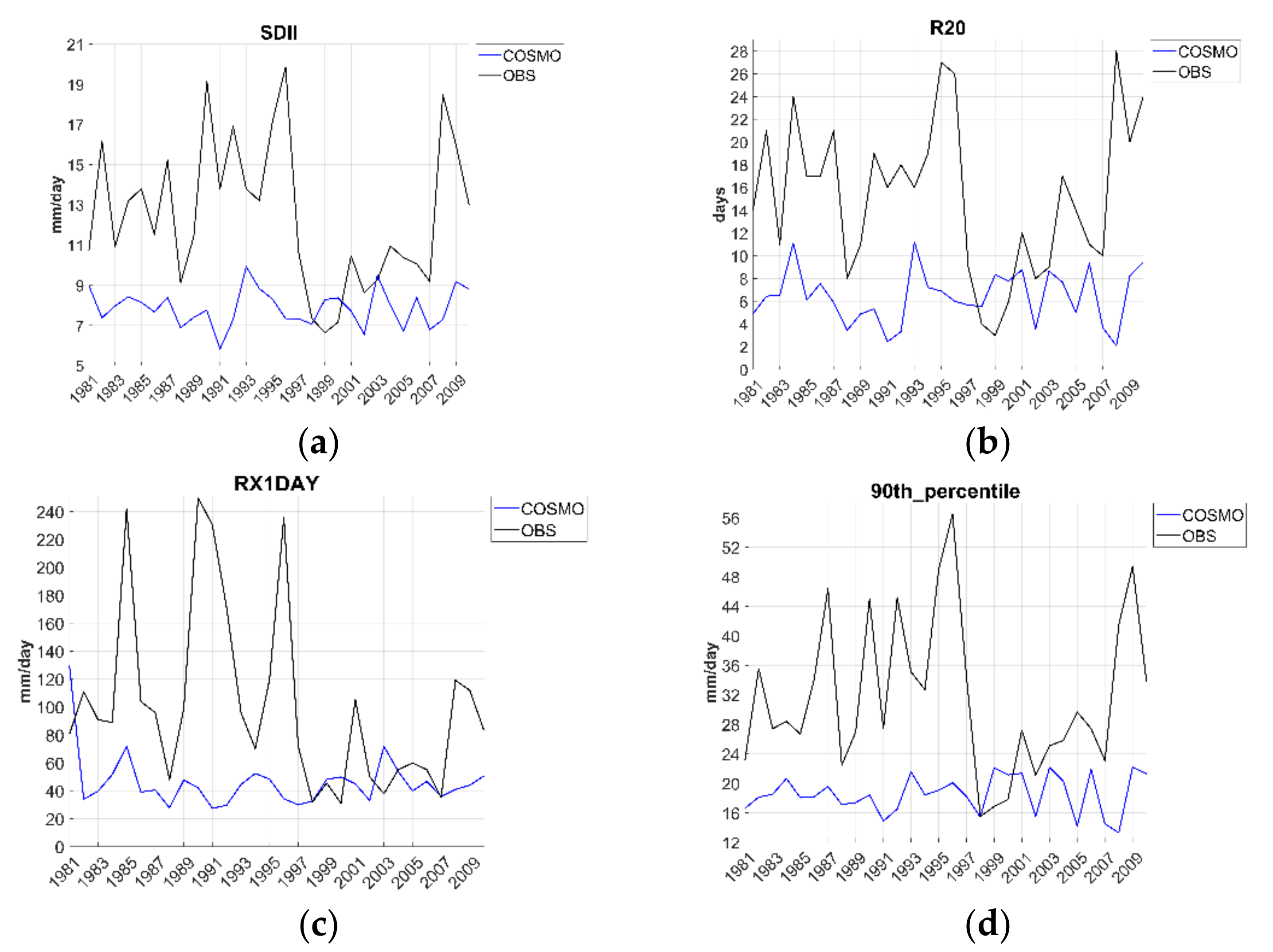
4.1. Model Evaluation

Modelled average values of 2-m temperature (T2m), precipitation and wind speed have been compared with observations for the period 1981–2010, in order to evaluate the capabilities of COSMO-CLM to simulate these basic variables over the area considered. Specifically, data generated by the model have been extracted considering the average value over a 3 × 3 grid box including the airport site.

Table 3. Mean observed value, mean bias and Root Mean Square Error (RMSE) of the model for maximum and minimum temperature, precipitation, and wind, averaged over the whole past period considered.

	Tmax (°C)	Tmin (°C)	Precipitation (mm/month)	Wind (m/s)
Mean observed val.	20.5	10.5	77	3.9
Mean bias	−1.5	−0.1	−22	−1.6
RMSE	1.9	0.6	41	1.5

shows the mean observational value, the mean bias, and Root Mean Square Error (RMSE) of the model for maximum and minimum temperature, precipitation, and wind, averaged over the whole past period considered. Figure 2a displays the annual cycles of daily maximum and minimum T2m for the model output and observational data. A good agreement is recorded for minimum values, while maximum values are generally underestimated, especially in winter months, since the simulated bare soil evaporation may be too high, thus creating a moist and cold bias, particularly during daytime [35]. Figure 2b displays the annual cycle of monthly precipitation: simulated values satisfactorily follow the course of the year, but a major underestimation is recorded over the whole year, with a peak in October. Figure 2c displays the annual cycle of daily wind speed in this case it is also well captured, but with an average negative bias of about 1.6 m/s, which is in line with the values affecting state-of-art NWP models, e.g., [36].

Modeled values of the selected EWIs were also compared with those calculated from the observational dataset. Figure 3 displays the time series of EWI temperature indicators for the model output and observational data over the historical period 1981–2010.

Table 4. Standard deviation and trend of the EWI considered over the historical period 1981–2010, for model and observational data.

	Standard Deviation		Trend
	COSMO	OBS	COSMO	OBS
TXx	2.0	1.7	0.06	−0.05
SU	3.4	2.8	0.10	−0.06
90p-Tmax	1.2	0.9	0.04	0.0
SDII	1.1	3.6	0.0	−0.07
R20	2.8	6.8	0.0	−0.06
Rx1day	28.1	63.8	−0.94	−2.48
90p-Prec	2.6	10.5	0.03	−0.02

shows the numerical values of standard deviation and trend of the EWI considered over the historical period, for modeling and observational data. These values reveal a good capability of the model in reproducing the observed trend of temperature indicators, with a fair agreement also in terms of standard deviation, as also confirmed by the time series of temperature indicators (Figure 3). The 90p-Tmax is generally underestimated. With regards to precipitation indicators, Table 4 shows a quite good agreement in terms of trend for SDII, R20, and 90p-Prec, while disagreements are recorded for standard deviation, especially for Rx1day. In fact, through analyzing the time series of EWI precipitation indicators over the historical period (Figure 4), it is evident that the most intense precipitation events are not reproduced by the model. However, it must be pointed out that the current values of the indicators provided by the model for the individual years cannot be used in a deterministic way, since the RCM is forced by a Global Model, and not by Reanalysis. In any case, it is known that COSMO-CLM has difficulties in localizing rain events: in fact, strong precipitation is often simulated in areas away from the site where the event really takes place, even at very high resolution (1 km) [18], and, of course, the situation gets worse when a resolution of approximately 8 km is employed. Moreover, it is worth noting that such discrepancies could also be due to inaccuracies of the observational dataset. In particular, events larger than 240 mm/day could be affected by measurement (or transcription) errors since, despite the data checks carried out by the sources at the origin, it may occur that a certain number of incorrect values escapes the controls and contributes to determine the value of indicators that are incorrect. Specifically, the observed time series have been checked using data from some nearby stations; even if these data are available only for limited periods, they are sufficient to see that some outliers recorded in Capodichino (e.g., in the years 1985, 1990) are not so evident in the other stations.

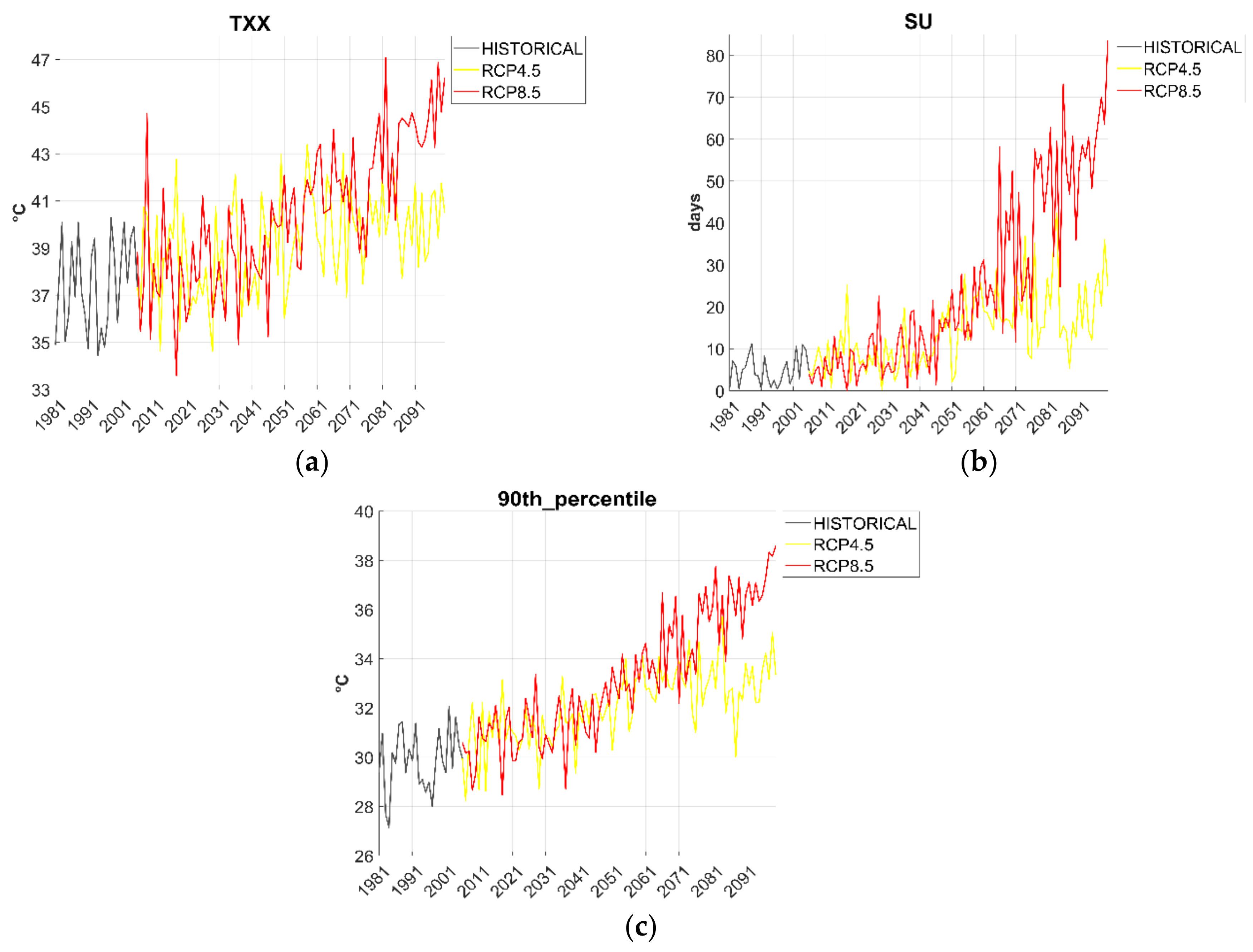
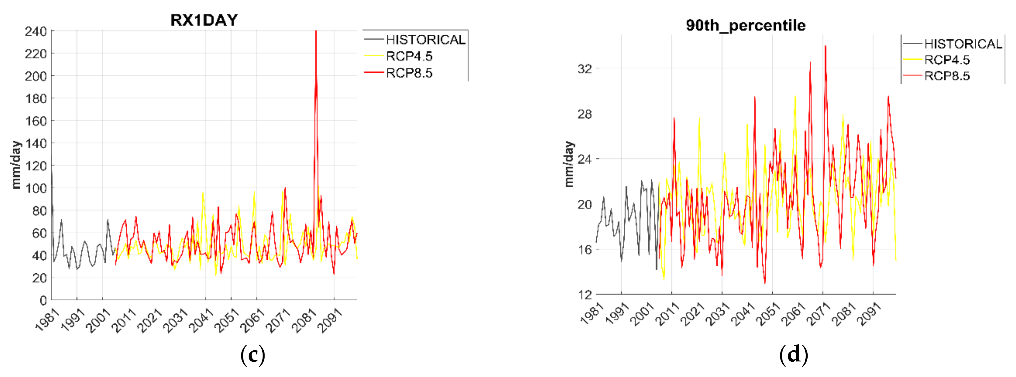
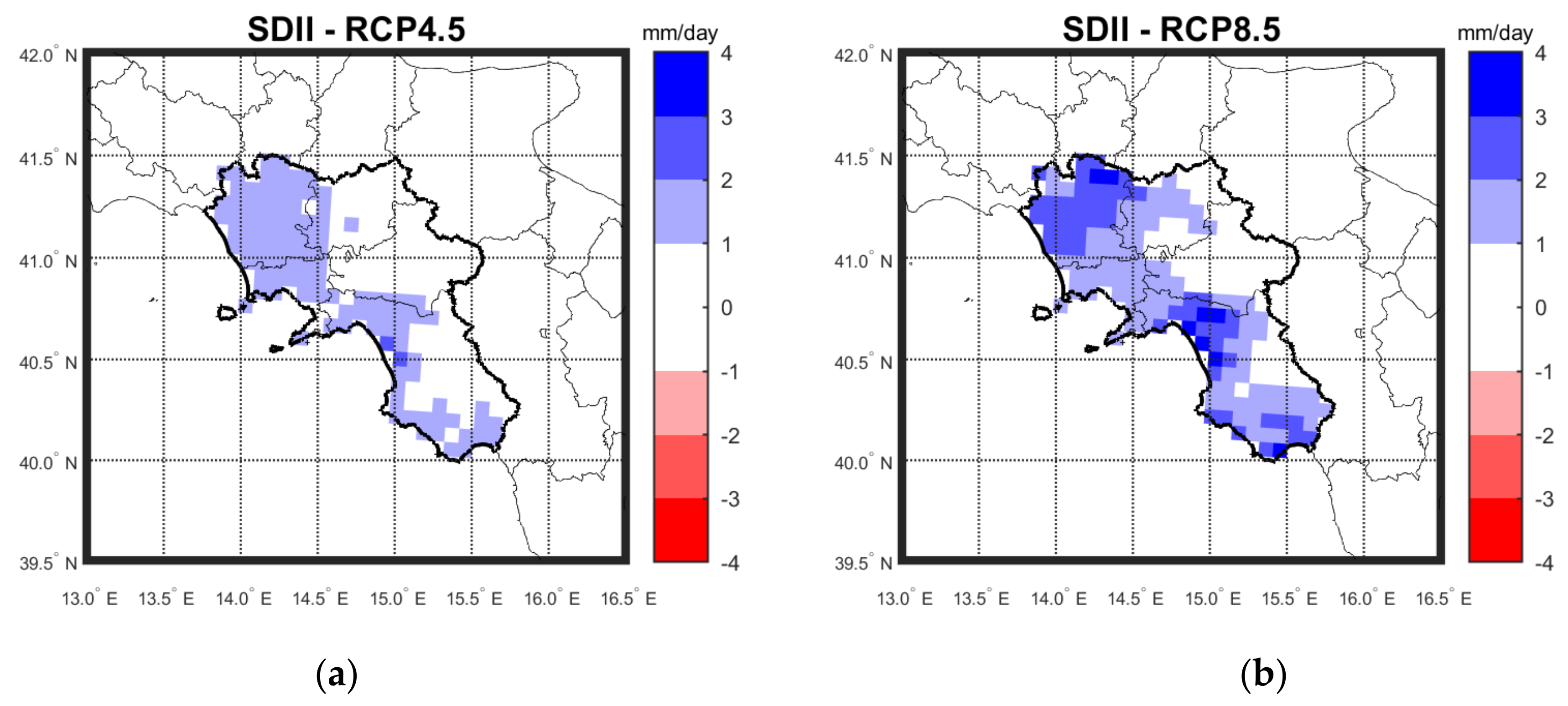
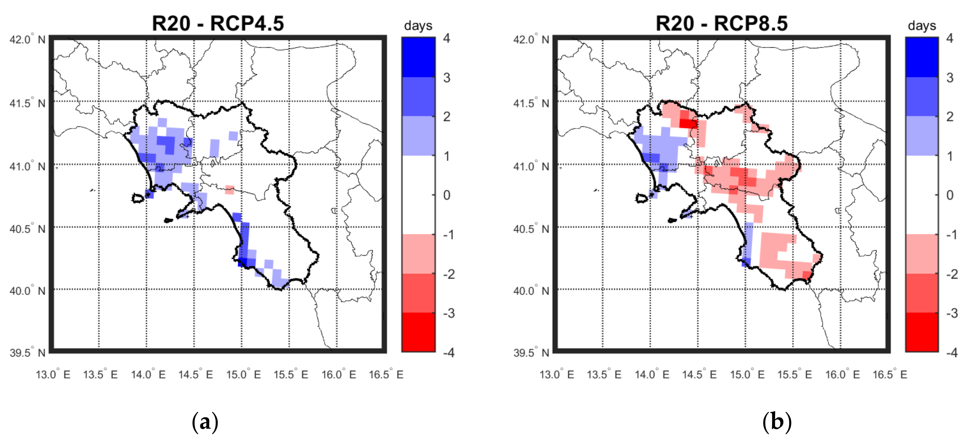
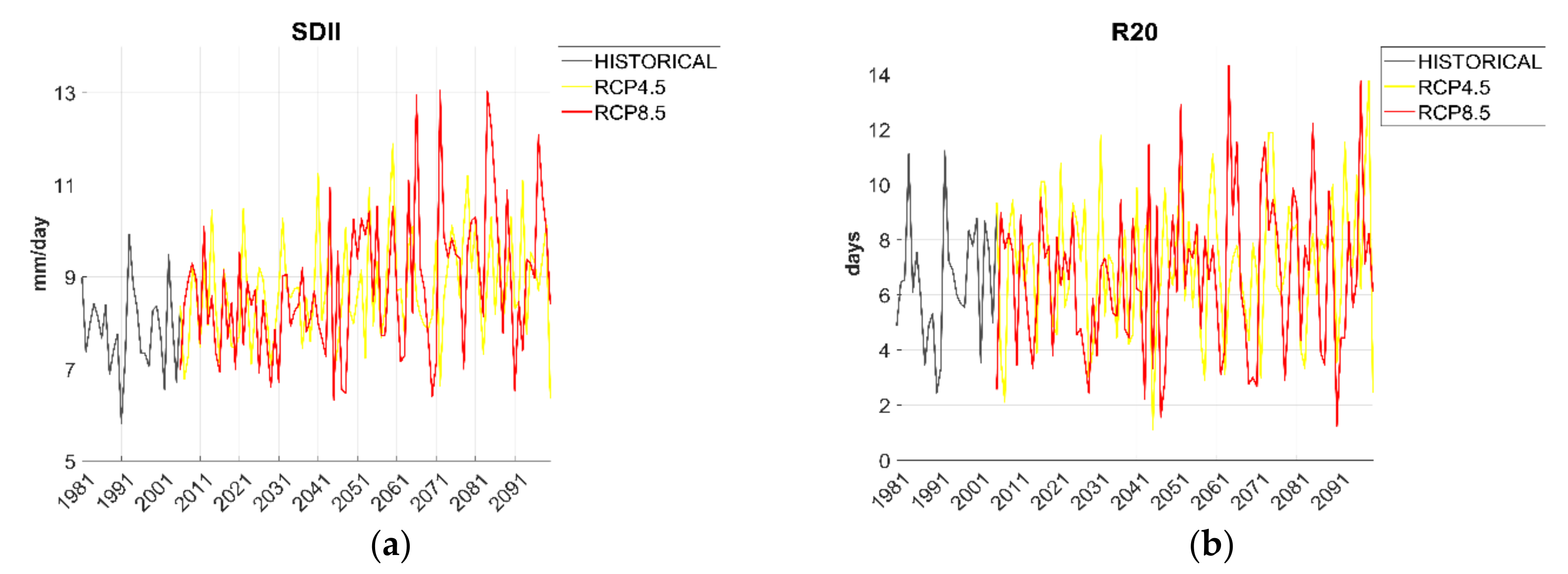
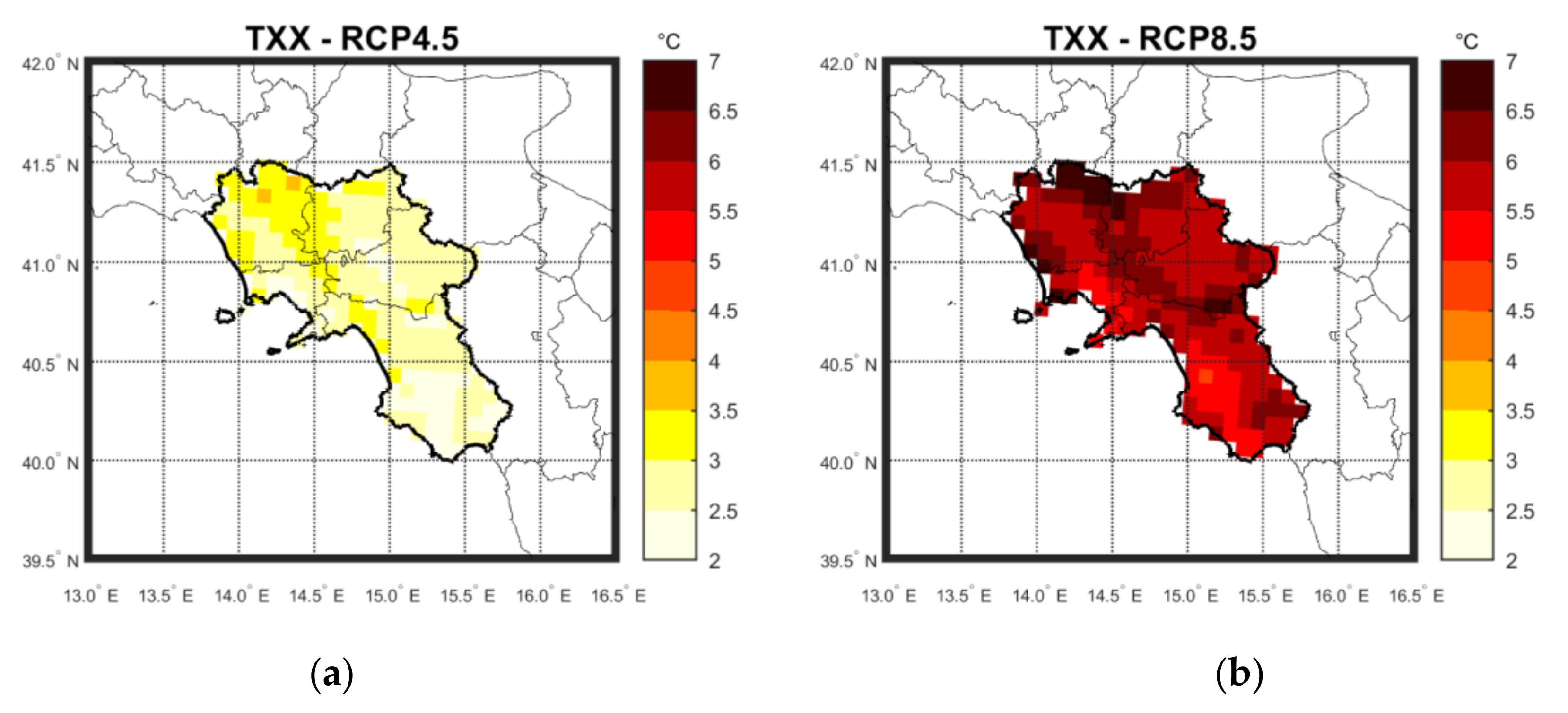
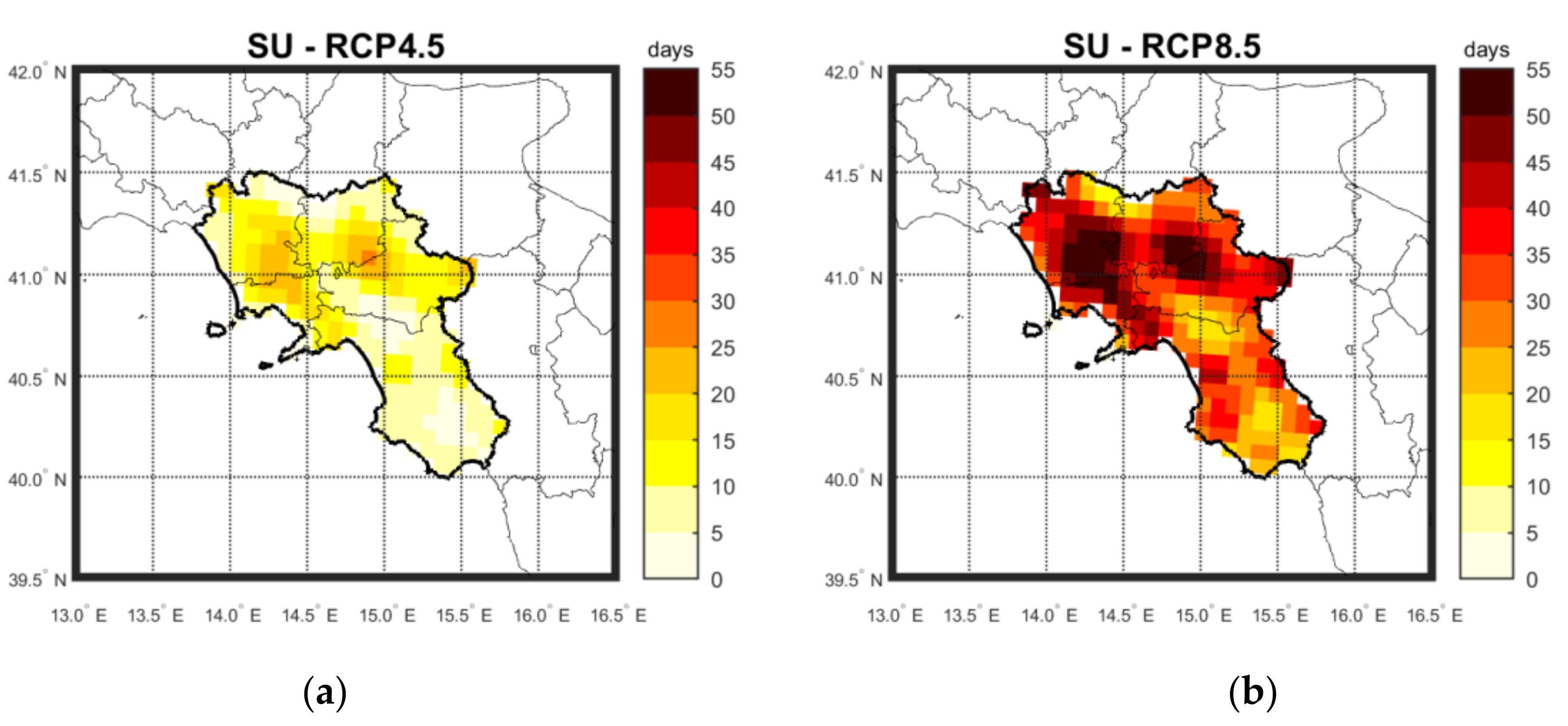
4.2. Climate Projections

Climate projections generated by COSMO-CLM have been investigated considering data averaged over a 3 × 3 grid box, including the airport site, and evaluating the indicators described in Table 2. All the time series shown in the following have been obtained over the historical period (1981–2005) and the future period (2006–2100) for both IPCC RCP4.5 and RCP8.5 scenarios. As already pointed out, the values of the indicators provided for the individual years cannot be used in a deterministic way, but they are only able to highlight the expected trends of the climate conditions over the 21st century.

Figure 5a shows the time series of TXx: both scenarios reveal an almost regular and gradual warming. Values of TXx in the past period range between 36 and 39 °C, while in the near future (i.e., until 2050), no relevant differences are recorded between the two scenarios, but trends differ significantly later on. In fact, the projected increases of TXx by 2100 with respect to the present climate range from 3 °C (percentage variation 7%) under RCP4.5 to 7 °C (15%) under RCP8.5. Figure 5b shows the time series of SU: a noticeable increasing trend is observed over the projected period for both scenarios, with peaks larger than 60 days/year at the end of the century under RCP8.5 (+800%). A perceptible growth is projected also for 90p-Tmax (Figure 5c), up to 7 °C under RCP8.5 (+20%). As regards precipitation indicators, Figure 6a shows the time series of SDII, revealing a slight increase of this indicator over the considered period under both scenarios; this result means that, in spite of the general reduction trend projected over Italy [27], precipitation in the rainy days will be more intense, as also confirmed by a slight increase of R20 over the considered period (Figure 6b). It could be related to the warmer climate of the area considered and the proximity to the sea, with the consequent increase of the amount of water that evaporates. Figure 6c shows that, for Rx1day, under both scenarios, peak values of about 90–100 mm/day are expected in the second half of XXI century (+29%). Finally, Figure 6d shows a slight growing trend also for 90p-Prec. The time series of FG has also been investigated, but they are not shown here, since no relevant variation trends are highlighted under both scenarios (the values of FG are always generally between 2 and 2.5 m/s over the period analyzed).

In order to have a wider frame of the expected changes of EWIs, maps over the whole Campania region for some indicators are provided. Specifically, Figure 7, Figure 8, Figure 9 and Figure 10 show the maps of the difference of the average value projected over the future period 2071–2100 (both scenarios), with respect to the average value over the past period 1981–2010, respectively for TXx, SU, SDII and R20.

The analysis of TXx and SU maps reveals that the sign of temperature climate change is the same for both scenarios, with strong increases under RCP8.5 over the whole area, and peaks over zones with specific climate and orographic features. The map of SDII shows that a growing trend is expected not only over the Naples area, but over about half of Campania region (the part closest to the sea), with increases ranging between 3 and 5 mm/day. Areas affected by increases of R20 are simulated over the northern coastal Campania areas, while reduction are projected over internal areas especially under RCP8.5. Maps of FG (not shown) do not reveal relevant variations for this indicator over the whole region, for both scenarios.

5. Discussion and Future Developments

Even if climatic extremes are conventionally modelled in engineering applications with three different Extreme Value Distributions (Weibull, Fréchet and Gumbel), in this work, climate indicators have been considered, since they have a wider context. The extreme climate indices defined by ETCCDI have promoted research of extreme climate events, and enhanced further research in model simulation and attribution of such events.

Model evaluation revealed that COSMO-CLM performances are satisfactory for temperature, while precipitation representation shows some deficiencies, which are in line or even lower than those of standard RCM models (e.g., EUROCORDEX simulations [37]). Moreover, it must be considered that the model is characterised by a resolution of 8 km, and that the validation is performed against data provided by a specific point station. This is a very ambitious evaluation, and it is not possible to expect a perfect overlapping between model output and observations, simply because those data are not referred to the same geographical point. In addition, rainfall underestimation (both in the climate and weather version of the model) in specific areas has been documented in several literature works, and especially difficulties in localizing rain events. Additional problems are probably due to sea surface temperature biases in proximity to the sea. The COSMO community is making a big effort in order to deal with this shortcoming, since precipitation is the most difficult atmospheric variable to be predicted with numerical models. Improvements in the simulation of convective rainfall, typical of spring months, could be achieved, increasing the spatial resolution and employing convection permitting schemes. As shown in [38], representation of heavy precipitation is enhanced when the resolution is increased from 11 to 3 km, with improvements even in the representation of sub-daily precipitation. Another source of uncertainty, especially in the case of extreme values (larger at small spatial case as in the present analysis) is related to the internal variability of the climate system, intrinsic to the chaotic nature of atmospheric and oceanic processes, limiting the predictability of the climate signal [39].

To overcome the large biases affecting climate models, a range of bias correction methods have been developed, which require long series of observational data. These are useful and powerful tools and are often applied, but generally a bias correction is recommended when climate data must be used as input for impact models, which cannot withstand with such large biases. The main aim of the present work is rather the definition of a risk assessment methodology based on the combination of the frequency and severity of meteorological hazards, describing expected trends (which are quite well reproduced, as shown in Table 4).

The extreme temperature indices considered over Napoli Capodichino project a significant increase, which is consistent with the general warming expected over the Campania region, and in general over Italy. Increases up to 7 °C, with respect to the present climate, could be reached at the end of the century, under the “business as usual” RCP8.5 scenario, with also relevant increases of SU, that could seriously jeopardize the airport’s functioning.

On the other side, an interesting and complex spatial pattern arises from the high-resolution simulation of precipitation indices, with an increase of their values over Capodichino, differently from previous simulations that projected a tendency towards drier conditions. In fact, this feature could be captured only by high resolution simulations, and not by the global models employed in earlier projections of extreme precipitation [40]. Of course, it would be interesting to analyze results for more airports in Italy, in order to see contrast and differences in the climate risk between airports in northern, central and southern Italy, since the analysis presented in [27] revealed that climate projections largely differ among zones and seasons (e.g., a large increase in precipitation is projected in winter over central and northern Italy). This comparison will be the subject of a future work.

Moreover, it is well known that projections of climate change are affected by uncertainty, because they are dependent on future anthropogenic scenarios that are uncertain, and due to the unavoidable not perfect representation of the climate system. A fundamental question related to the reliability of climate projections is whether they may be influenced by the presence of biases in model simulations. This question has been addressed in many studies, and the general opinion (e.g., [41]) is that biases in the base and projected years are fairly consistent, suggesting that projection changes provide a reasonable bias removal. That said, the reliability of projections might be improved by using multi-model ensembles, weighting single elements with some measure of model skills [42]. Moreover, model ensembles are needed also for the uncertainty quantification, which is fundamental in decision making processes. Considering the huge computational costs required, it is necessary that ensembles use a common framework to achieve robust and useful conclusions in projecting future regional climate change, as addressed by the EURO-CORDEX project [37].

In order to identify the potential risks regarding climate change, the previous analysis must be complemented by a climate change risk assessment. The EWI indices considered in this study are not only suited as assessment tools in multiple sectors, but also as metrics to be aggregated as composite indicators for risk assessment studies (an example of application in the form of a Climate Risk Index is shown in [43]). The result is generally referred to as risk exposure, and is a measure of the risk that the airport faces in relation to the climate impact. Considering that risks and exposure are generally based on a defined timeframe, risks may increase if a longer timeframe is applied. The account for risk exposure is generally performed by using the default ICAO (International Civil Aviation Organization) risk matrix (

Table 5. The ICAO risk matrix.

	Catastrophic	Hazardous	Major	Minor	Negligible
Frequent	5A	5B	5C	5D	5E
Occasional	4A	4B	4C	4D	4E
Remote	3A	3B	3C	3D	3E
Improbable	2A	2B	2C	2D	2E
Extremely improbable	1A	1B	1C	1D	1E

) that provides a risk index by combining probability and severity. Couples of a number and a letter are used, corresponding respectively to the probability of negative outcome and to the severity of the most likely negative outcome. The matrix is generally a 5 × 5 grid organized in colors, with green color representing low risk, yellow representing medium risk and red equals to high risk.

Concerning the severity of events, a catastrophic event means that the equipment is destroyed and/or that multiple deaths were recorded, a hazardous event implies major damages and/or loss of one life or serious injury, and a major event implies significant damage to equipment and/or injuries (serious incident). Finally, a minor event implies slight degradation of mission performance, while if the event is classified as negligible, there are no significant consequences.

Every single component of the airport is subject to a level of risk given by the product of the occurrence probability of the climate change by its impact on the airport component. The result of the methodology can be summarized in a final risk matrix, where the lines of the matrix represent the different airport components (for example runways, taxiways, apron, car parks, accesses to the airport, etc.) and the columns represent the different factors of climate change that create impacts on the infrastructure. The value of each cell will identify the level of risk associated to each airport component based on the climate scenario and period chosen. This matrix could aid in identifying the strength and weaknesses of the airport to improve the climate change resilience, in order to support stakeholders in the identification of suitable adaptation strategies. According with [14], specific indicators must be used as proxies for identifying not only hazards, but also exposure and vulnerability characteristics. Those indicators are linked to physical (such as age, percentage of impervious surfaces) and socioeconomic features (e.g., air traffic, number of passengers). However, a rigorous definition of this matrix is beyond the purposes of the present study, and will be addressed in a future complementary work.

References

1. Scorzini, A.R.; Di Bacco, M.; Leopardi, M. Recent trends in daily temperature extremes over the central Adriatic region of Italy in a Mediterranean climatic context. Int. J. Clim. 2018, 38, e741–e757. [Google Scholar] [CrossRef]
2. Donat, M.G.; Alexander, L.; Yang, H.; Durre, I.; Vose, R.; Dunn, R.; Willett, K.M.; Aguilar, E.; Brunet, M.; Caesar, J.; et al. Updated analyses of temperature and precipitation extreme indices since the beginning of the twentieth century: The HadEX2 dataset. J. Geophys. Res. Atmos. 2013, 118, 2098–2118. [Google Scholar] [CrossRef]
3. European Environment Agency (EEA). Climate change adaptation and disaster risk reduction in Europe Enhancing Coherence of the Knowledge Base, Policies and Practices; EEA Report 15/17; European Environment Agency: Copenhagen, Denmark, 2017. [Google Scholar]
4. IPCC. Climate Change 2014: Synthesis Report; Contribution of Working Groups I, II and III to the Fifth Assessment Report of the Intergovernmental Panel on Climate Change, Core Writing Team, R.K. Pachauri and L.A. Meyer; IPCC: Geneva, Switzerland, 2014. [Google Scholar]
5. IPCC. Climate Change 2021: The Physical Science Basis; Masson-Delmotte, V.P., Zhai, A., Pirani, S.L., Connors, C., Péan, S., Berger, N., Caud, Y., Chen, L., Goldfarb, M.I., Gomis, M., et al., Eds.; Contribution of Working Group I to the Sixth Assessment Report of the Intergovernmental Panel on Climate Change; Cambridge University Press: Cambridge, UK; New York, NY, USA, 2021; in press. [Google Scholar]
6. Wilbanks, T.; Fernandez, L. Climate Change and Infrastructure, Urban Systems, and Vulnerabilities; Technical Report for the U.S. Department of Energy in Support of the National Climate Assessment; Island Press: Washington, DC, USA, 2012. [Google Scholar]
7. Christodoulou, A.; Demirel, H. Impacts of Climate Change on Transport: A Focus on Airports, Seaports and Inland Waterways; EUR 28896 EN; Publications Office of the European Union: Luxembourg, 2018; ISBN 978-92-79-97039-9. [Google Scholar]
8. EUROCONTROL. Challenges of Growth 2013—Task 8: Climate Change Risk and Resilience, STATFOR, EUROCONTROL. 2013. Available online: https://www.eurocontrol.int/sites/default/files/article/content/documents/official-documents/reports/201303-challenges-of-growth-2013-task-8.pdf (accessed on 12 July 2021).
9. ICAO. Environment Report of International Civil Aviation Organization—Destination Green, The Next Chapter. 2019. Available online: https://www.icao.int/environmental-protection/Pages/envrep2019.aspx (accessed on 12 July 2021).
10. Burbidge, R. Adapting aviation to a changing climate: Key priorities for action. J. Air Transp. Manag. 2018, 71, 167–174. [Google Scholar] [CrossRef]
11. Gratton, G.; Padhra, A.; Rapsomanikis, S.; Williams, P. The impacts of climate change on Greek airports. Clim. Chang. 2020, 160, 219–231. [Google Scholar] [CrossRef] [Green Version]
12. Lelieveld, J.; Hadjinicolaou, P.; Kostopoulou, E.; Chenoweth, J.; El Maayar, M.; Giannakopoulos, C.; Hannides, C.; Lange, M.A.; Tanarhte, M.; Tyrlis, E.; et al. Climate change and impacts in the Eastern Mediterranean and the Middle East. Clim. Chang. 2012, 114, 667–687. [Google Scholar] [CrossRef] [Green Version]
13. Ciscar, J.C.; Ibarreta, D.; Soria, A. Climate Impacts in Europe: Final Report of the JRC PESETA III Project. 2018. Available online: https://www.preventionweb.net/files/61911_pesetaiiifinalreport.pdf (accessed on 12 July 2021).
14. De Vivo, C.; Ellena, M.; Capozzi, V.; Budillon, G.; Mercogliano, P. Risk assessment framework for Mediterranean airports: A focus on extreme temperatures and precipitations and sea level rise. Nat. Hazards 2021. [Google Scholar] [CrossRef]
15. Lopez, A. Vulnerability of Airports on Climate Change: An Assessment Methodology. Transp. Res. Procedia 2016, 14, 24–31. [Google Scholar] [CrossRef] [Green Version]
16. Coffel, E.D.; Thompson, T.R.; Horton, R.M. The impacts of rising temperatures on aircraft takeoff performance. Clim. Chang. 2017, 144, 381–388. [Google Scholar] [CrossRef]
17. Stephenson, D.B. Definition, diagnosis, and origin of extreme weather and climate events. In Climate Extremes and Society; Diaz, H.F., Murnane, R.J., Eds.; Cambridge University Press: Cambridge, UK; New York, NY, USA, 2008; pp. 11–22. [Google Scholar]
18. Bucchignani, E.; Mercogliano, P. Performance Evaluation of High-Resolution Simulations with COSMO over South Italy. Atmosphere 2021, 12, 45. [Google Scholar] [CrossRef]
19. Burbidge, R. Adapting European Airports to a Changing Climate. Transp. Res. Procedia 2016, 14, 14–23. [Google Scholar] [CrossRef] [Green Version]
20. Thomas, C.; McCarthy, R.; Lewis, K.; Boucher, O.; Hayward, J.; Owen, B.; Liggings, F. Challenges to Growth Environmental Update Study; EUROCONTROL: Brussels, Belgium, 2009. [Google Scholar]
21. Williams, P.D. Transatlantic flight times and climate change. Environ. Res. Lett. 2016, 11, 24008. [Google Scholar] [CrossRef]
22. Williams, P.; Joshi, M. Intensification of winter transatlantic aviation turbulence in response to climate change. Nat. Clim. Chang. 2013, 3, 644–648. [Google Scholar] [CrossRef]
23. Williams, P.D. Increased light, moderate, and severe clear-air turbulence in response to climate change. Adv. Atmos. Sci. 2017, 34, 576–586. [Google Scholar] [CrossRef] [Green Version]
24. Dejmal, K.; Novotny, J. Application of Fog Stability Index for significantly reduced visibility forecasting in the Czech Republic. In Recent Advances in Fluid Mechanics and Heat Mass Transfer; Lazard, M., Ed.; WSEAS Press: Athens, Greece, 2011; pp. 317–320. [Google Scholar]
25. Stoelinga, M.T.; Warner, T.T. Nonhydrostatic, Mesobeta-Scale Model Simulations of Cloud Ceiling and Visibility for an East Coast Winter Precipitation Event. J. Appl. Meteorol. 1999, 38, 385–404. [Google Scholar] [CrossRef]
26. Rockel, B.; Will, A.; Hense, A. The Regional Climate Model COSMO-CLM (CCLM). Meteorol. Z. 2008, 17, 347–348. [Google Scholar] [CrossRef]
27. Bucchignani, E.; Montesarchio, M.; Zollo, A.L.; Mercogliano, P. High-resolution climate simulations with COSMO-CLM over Italy: Performance evaluation and climate projections for the 21st century. Int. J. Cliamatol. 2016, 36, 735–756. [Google Scholar] [CrossRef]
28. Scoccimarro, E.; Gualdi, S.; Bellucci, A.; Sanna, A.; Fogli, P.G.; Manzini, E.; Vichi, M.; Oddo, P.; Navarra, A. Effects of Tropical Cyclones on Ocean Heat Transport in a High-Resolution Coupled General Circulation Model. J. Clim. 2011, 24, 4368–4384. [Google Scholar] [CrossRef] [Green Version]
29. Moss, R.H.; Edmonds, J.A.; Hibbard, K.A.; Manning, M.R.; Rose, S.K.; van Vuuren, D.P.; Carter, T.R.; Emori, S.; Kainuma, M.; Kram, T.; et al. The next generation of scenarios for climate change research and assessment. Nature 2010, 463, 747–756. [Google Scholar] [CrossRef] [PubMed]
30. Van Vuuren, D.P.; Edmonds, J.; Kainuma, M.; Riahi, K.; Thomson, A.; Hibbard, K.; Hurtt, G.C.; Kram, T.; Krey, V.; Lamarque, J.-F.; et al. The representative concentration pathways: An overview. Clim. Chang. 2011, 109, 5–31. [Google Scholar] [CrossRef]
31. WMO. Guidelines on Analysis of Extremes in a Changing Climate in Support of Informed Decisions for Adaptation; Technical Report WCDMP No. 72, WMO/TD-No. 1500; WMO: Geneva, Switzerland, 2009. [Google Scholar]
32. Fischer, T.; Menz, C.; Su, B.; Scholten, T. Simulated and projected climate extremes in the Zhujiang River Basin, South China, using the regional climate model COSMO-CLM. Int. J. Clim. 2013, 33, 2988–3001. [Google Scholar] [CrossRef]
33. Zollo, A.L.; Rillo, V.; Bucchignani, E.; Montesarchio, M.; Mercogliano, P. Extreme temperature and precipitation events over Italy: Assessment of high-resolution simulations with COSMO-CLM and future scenarios. Int. J. Clim. 2016, 36, 987–1004. [Google Scholar] [CrossRef] [Green Version]
34. Desiato, F.; Lena, F.; Toreti, A. SCIA: A system for a better knowledge of the Italian climate. Boll. Geoff. Theory Appl. 2007, 48, 351–358. [Google Scholar]
35. Schulz, J.-P.; Vogel, G. Improving the Processes in the Land Surface Scheme TERRA: Bare Soil Evaporation and Skin Temperature. Atmosphere 2020, 11, 513. [Google Scholar] [CrossRef]
36. Heppelmann, T.; Steiner, A.; Vogt, S. Application of numerical weather prediction in wind power forecasting: Assessment of the diurnal cycle. Meteorol. Z. 2017, 26, 319–331. [Google Scholar] [CrossRef]
37. Jacob, D.; Teichmann, C.; Sobolowski, S.; Katragkou, E.; Anders, I.; Belda, M.; Benestad, R.; Boberg, F.; Buonomo, E.; Cardoso, R.M.; et al. Regional climate downscaling over Europe: Perspectives from the EURO-CORDEX community. Reg. Environ. Chang. 2020, 20, 1–20. [Google Scholar] [CrossRef]
38. Adinolfi, M.; Raffa, M.; Reder, A.; Mercogliano, P. Evaluation and Expected Changes of Summer Precipitation at Convection Permitting Scale with COSMO-CLM over Alpine Space. Atmosphere 2021, 12, 54. [Google Scholar] [CrossRef]
39. Martel, J.-L.; Mailhot, A.; Brissette, F.; Caya, D. Role of Natural Climate Variability in the Detection of Anthropogenic Climate Change Signal for Mean and Extreme Precipitation at Local and Regional Scales. J. Clim. 2018, 31, 4241–4263. [Google Scholar] [CrossRef]
40. Giorgi, F.; Lionello, P. Climate change projections for the Mediterranean region. Glob. Planet. Chang. 2008, 63, 90–104. [Google Scholar] [CrossRef]
41. Maurer, E.P.; Das, T.; Cayan, D.R. Errors in climate model daily precipitation and temperature output: Time invariance and implications for bias correction. Hydrol. Earth Syst. Sci. 2013, 17, 2147–2159. [Google Scholar] [CrossRef] [Green Version]
42. Knutti, R.; Abramowitz, G.; Collins, M.; Eyring, V.; Gleckler, P.J.; Hewitson, B.; Mearns, L. Good practice guidance paper on assessing and combining multi model climate projections. In Meeting Report of the Intergovernmental Panel on Climate Change Expert Meeting on Assessing and Combining Multi Model Climate Projections; Stocker, T.F., Qin, D., Plattner, G.K., Tignor, M., Midgley, P.M., Eds.; IPCC Working Group I Technical Support Unit, University of Bern: Bern, Switzerland, 2010. [Google Scholar]
43. Mysiak, J.; Torresan, S.; Bosello, F.; Mistry, M.; Amadio, M.; Marzi, S.; Furlan, E.; Sperotto, A. Climate risk index for Italy. Philos. Trans. R. Soc. A Math. Phys. Eng. Sci. 2018, 376, 20170305. [Google Scholar] [CrossRef] [PubMed]
Figure 1. Geographical Location of Napoli Capodichino Airport in Southern Italy.
Earth 02 00058 g001
Figure 2. Annual cycle of (a) daily maximum and minimum 2-m temperature (°C), (b) precipitation, (c) wind speed for the COSMO model output and observational data.
Earth 02 00058 g002
Figure 3. Time series of (a) TXx, (b) SU, and (c) 90p-Tmax for the model output and observational data over the historical period 1981–2010.
Earth 02 00058 g003
Figure 4. Time series of (a) SDII, (b) R20, (c) Rx1day, and (d) 90p-Prec for the model output of the simulation and observational data over the historical period 1981–2010.
Earth 02 00058 g004
Figure 5. Time series of (a) TXx, (b) SU and (c) 90p-Tmax under IPCC RCP4.5 and RCP8.5 scenarios.
Earth 02 00058 g005
Figure 6. Time series of (a) SDII, (b) R20, (c) Rx1day, (d) 90p-Prec under IPCC RCP4.5 and RCP8.5 scenarios.
Earth 02 00058 g006aEarth 02 00058 g006b
Figure 7. Maps of the difference of the average TXx value projected over the future period 2071–2100, with respect to the past period 1981–2010 under (a) RCP4.5 and (b) RCP8.5.
Earth 02 00058 g007
Figure 8. Maps of the difference of the average SU value projected over the future period 2071–2100, with respect to the past period 1981–2010 under (a) RCP4.5 and (b) RCP8.5.
Earth 02 00058 g008
Figure 9. Maps of the difference of the average SDII value projected over the future period 2071–2100, with respect to the past period 1981–2010 under (a) RCP4.5 and (b) RCP8.5.
Earth 02 00058 g009
Figure 10. Maps of the difference of the average R20 value projected over the future period 2071–2100, with respect to the past period 1981–2010 under (a) RCP4.5 and (b) RCP8.5.
Earth 02 00058 g010