Land Cover Change and Soil Carbon Regulating Ecosystem Services in the State of South Carolina, USA

 ,
,  , ,
, ,  , and
, and
Abstract
:1. Introduction
2. Materials and Methods
2.1. Spatial Analysis
2.2. The Accounting Framework
3. Results
3.1. Land Cover Change in South Carolina
3.2. Land Cover Change and Soil Carbon Regulating Ecosystem Services in South Carolina
3.3. Land Cover Change and Soil Carbon Regulating Ecosystem Services by Soil Order, County, and Region
4. Discussion
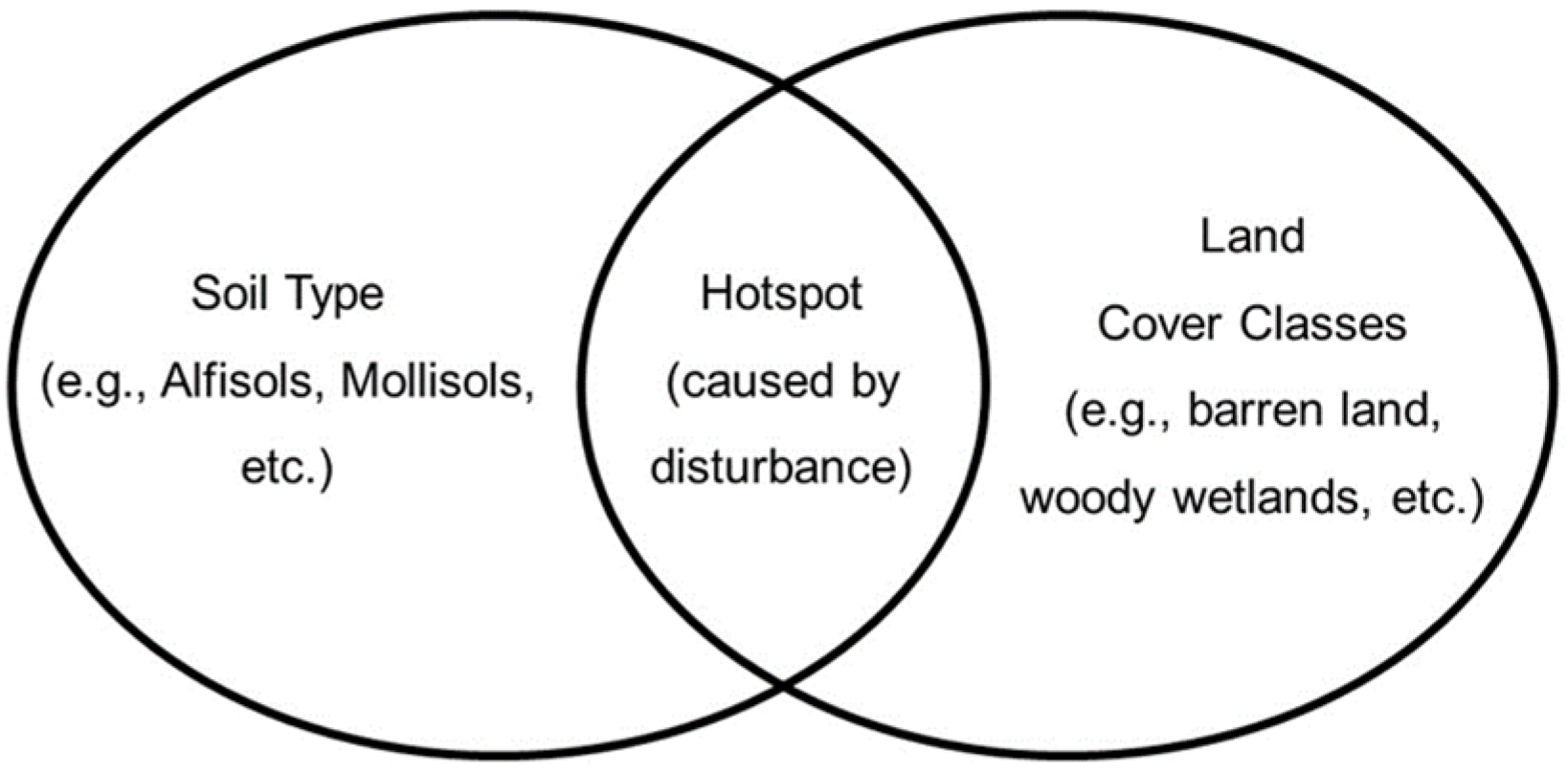
4.1. Determining “Hotspots” of Social Costs of C from Land Cover Change and Pedodiversity
4.2. Determining Potential for C Sequestration Using LULC and Pedodiversity
4.3. Significance of Results for South Carolina
- Inventory of South Carolina’s Greenhouse Gas Emissions. Current SC GHG inventories do not include soil and LULC analysis. This study quantified and valued the soil C regulating ES for SOC, SIC, and TSC for the state of South Carolina by soil type and LULC. According to the final report by the South Carolina Climate, Energy, and Commerce Committee [42]: “South Carolina’s gross emissions of GHGs grew by 39% between 1990 and 2005, twice the national average of 16%. South Carolina’s emissions growth was driven by the growth of its population and many other factors. In addition, the state’s emissions on a per-capita basis increased by about 15% between 1990 and 2005, while U.S. per-capita emissions declined slightly (2%) over this period due to many other factors. South Carolina’s gross GHG emissions are projected to rise fairly steeply to about 125 MMtCO2e by 2025, or 87% over 1990 levels.” Areas that developed in South Carolina over a 15-year time period were evaluated by the combination of soil type, LULC, and county to calculate the potential realized SC-CO2 from this land conversion. By identifying these potential SC-CO2 hotspots, future land conversions could be reduced to help lower future greenhouse gas emissions.
- Agriculture, Forestry and Waste Management (AFW):
- Transportation and Land Use (TLU):
- Cross-Cutting (CC) Issues:
5. Conclusions
Author Contributions
Funding
Acknowledgments
Conflicts of Interest
Glossary
| ED | Ecosystem disservices |
| ES | Ecosystem services |
| EPA | Environmental Protection Agency |
| SC-CO2 | Social cost of carbon emissions |
| LULC | Land cover classes |
| SDGs | Sustainable Development Goals |
| SOC | Soil organic carbon |
| SIC | Soil inorganic carbon |
| SOM | Soil organic matter |
| SSURGO | Soil Survey Geographic Database |
| TSC | Total soil carbon |
| USDA | United States Department of Agriculture |
| U.S.A. | United States of America |
References
- Pereira, P.; Bogunovic, I.; Muñoz-Rojas, M.; Brevik, E.C. Soil ecosystem services, sustainability, valuation and management. Curr. Opin. Environ. Sci. Health 2018, 5, 7–13. [Google Scholar] [CrossRef]
- Zhang, W.; Ricketts, T.H.; Kremen, C.; Carney, K.; Swinton, S.M. Ecosystem services and dis-services to agriculture. Ecol. Econ. 2007, 64, 253–260. [Google Scholar] [CrossRef] [Green Version]
- Mikhailova, E.A.; Groshans, G.R.; Post, C.J.; Schlautman, M.A.; Post, G.C. Valuation of soil organic carbon stocks in the contiguous United States based on the avoided social cost of carbon emissions. Resources 2019, 8, 153. [Google Scholar] [CrossRef] [Green Version]
- Groshans, G.R.; Mikhailova, E.A.; Post, C.J.; Schlautman, M.A.; Zhang, L. Determining the value of soil inorganic carbon stocks in the contiguous United States based on the avoided social cost of carbon emissions. Resources 2019, 8, 119. [Google Scholar] [CrossRef] [Green Version]
- Groshans, G.R.; Mikhailova, E.A.; Post, C.J.; Schlautman, M.A.; Zurqani, H.A.; Zhang, L. Assessing the value of soil inorganic carbon for ecosystem services in the contiguous United States based on liming replacement costs. Land 2018, 7, 149. [Google Scholar] [CrossRef] [Green Version]
- Houghton, R.A.; Nassikas, A.A. Global and regional fluxes of carbon from land use and land cover change 1850–2015. Glob. Biogeochem. Cycles 2017, 31, 456–472. [Google Scholar] [CrossRef]
- Zamanian, K.; Zhou, J.; Kuzyakov, Y. Soil carbonates: The unaccounted, irrecoverable carbon source. Geoderma 2021, 384, 114817. [Google Scholar] [CrossRef]
- Burkhard, B.; Kroll, F.; Nedkov, S.; Muller, F. Mapping ecosystem service supply, demand, and budgets. Ecol. Indic. 2012, 21, 17–29. [Google Scholar] [CrossRef]
- Sleeter, B.M.; Sohl, T.L.; Loveland, T.R.; Auch, R.F.; Acevedo, W.; Drummond, M.A.; Sayler, K.L.; Stehman, S.V. Land-cover change in the conterminous United States from 1973 to 2000. Glob. Environ. Chang. 2013, 23, 733–748. [Google Scholar] [CrossRef] [Green Version]
- Zhang, F.; Xu, N.; Wang, C.; Wu, F.; Chu, X. Effects of land use and land cover change on carbon sequestration and adaptive management in Shanghai, China. Phys. Chem. Earth 2020, 120, 102948. [Google Scholar] [CrossRef]
- Mikhailova, E.A.; Post, C.J.; Schlautman, M.A.; Post, G.C.; Zurqani, H.A. Determining farm-scale site-specific monetary value of “soil carbon hotspots” based on avoided social costs of CO2 emissions. Cogent Environ. Sci. 2020, 6, 1817289. [Google Scholar] [CrossRef]
- Brown, M.G.; Quinn, J.E. Zoning does not improve the availability of ecosystem services in urban watersheds. A case study from Upstate South Carolina, USA. Ecosyst. Serv. 2018, 34, 254–265. [Google Scholar] [CrossRef]
- Nelson, E.; Ennaanay, D.; Wolny, S.; Olwero, N.; Vigerstol, K.; Penning-ton, D.; Mendoza, G.; Aukema, J.; Foster, J.; Forrest, J.; et al. InVEST 3.6.0 User’s Guide. The Natural Capital Project. 2018, Stanford University, University of Minnesota, The Nature Conservancy, and World Wildlife Fund. Available online: http://data.naturalcapitalproject.org/nightly-build/invest-usersguide/InVEST_3.6.0_Documentation.pdf (accessed on 12 December 2020).
- Bétard, F.; Peulvast, J. Geodiversity hotspots: Concept, method and cartographic application for geoconservation purposes at a regional scale. Environ. Manag. 2019, 63, 822–834. [Google Scholar] [CrossRef]
- Mikhailova, E.A.; Zurqani, H.A.; Post, C.J.; Schlautman, M.A.; Post, G.C.; Lin, L.; Hao, Z. Soil carbon regulating ecosystem services in the state of South Carolina. Land 2021, 10, 309. [Google Scholar] [CrossRef]
- EPA. The Social Cost of Carbon. EPA Fact Sheet. 2016. Available online: https://19january2017snapshot.epa.gov/climatechange/social-cost-carbon_.html (accessed on 15 March 2019).
- Guo, Y.; Amundson, R.; Gong, P.; Yu, Q. Quantity and spatial variability of soil carbon in the conterminous United States. Soil Sci. Soc. Am. J. 2006, 70, 590–600. [Google Scholar] [CrossRef] [Green Version]
- Multi-Resolution Land Characteristics Consortium (MRLC). Available online: https://www.mrlc.gov/ (accessed on 1 March 2021).
- ESRI. ArcMap 10.7. Available online: https://support.esri.com/en/products/desktop/arcgis-desktop/arcmap/10-7-1 (accessed on 1 March 2021).
- Soil Survey Staff, Natural Resources Conservation Service, United States Department of Agriculture. Soil Survey Geographic (SSURGO) Database for South Carolina. Available online: https://www.nrcs.usda.gov/wps/portal/nrcs/detail/soils/survey/?cid=nrcs142p2_053627 (accessed on 1 March 2021).
- U.S. Geological Survey. The National Land Cover Database; Report, Series Number 2012–3020; U.S. Geological Survey: Reston, VA, USA, 2012.
- Werts, J.D.; Mikhailova, E.A.; Post, C.J.; Sharp, J.L. Sediment pollution assessment of abandoned residential developments using remote sensing and GIS. Pedosphere 2013, 23, 39–47. [Google Scholar] [CrossRef]
- Mechtensimer, S.; Toor, G.S. Septic systems contribution to phosphorus in shallow groundwater: Field-scale studies using conventional drainfield designs. PLoS ONE 2017, 12, e0170304. [Google Scholar] [CrossRef] [Green Version]
- Sayler, K.L.; Acevedo, W.; Taylor, J.L. (Eds.) Status and Trends of Land Change in the Eastern United States—1973 to 2000: U.S. Geological Survey Professional Paper 1794–D; USGS Publications Warehouse: Reston, VA, USA, 2016; p. 195. [Google Scholar] [CrossRef] [Green Version]
- Arnold, C.; Wilson, E.; Hurd, J.; Civco, D. 30 years of land cover change in Connecticut, USA: A case study of long-term research, dissemination of results, and their use in land use planning and natural resource conservation. Land 2020, 9, 255. [Google Scholar] [CrossRef]
- Galang, M.A.; Markewitz, D.; Morris, L.A.; Bussell, P. Land use change and gully erosion in the Piedmont region of South Carolina. J. Soil Water Conserv. 2007, 62, 122–129. [Google Scholar]
- Coughlan, M.R.; Nelson, D.R.; Lonneman, M.; Block, A.E. Historical land use dynamics in the highly degraded landscape of the Calhoun Critical Zone Observatory. Land 2017, 6, 32. [Google Scholar] [CrossRef] [Green Version]
- Li, J.; Chen, H.; Zhang, C.; Pan, T. Variations in ecosystem service value in response to land use/land cover changes in Central Asia from 1995–2035. Peer J. 2019, 7, e7665. [Google Scholar] [CrossRef] [PubMed]
- Coupe, R.H.; Barlow, J.R.B.; Capel, P.D. Complexity of human and ecosystem interactions in an agricultural landscape. Environ. Dev. 2012, 4, 88–104. [Google Scholar] [CrossRef]
- Wickham, J.; Stehman, S.V.; Sorenson, D.G.; Gass, L.; Dewitz, J.A. Thematic accuracy assessment of the NLCD 2016 land cover for the conterminous United States. Remote Sens. Environ. 2021, 257, 112357. [Google Scholar] [CrossRef]
- Zhu, Z.; Zhang, J.; Yang, Z.; Aljaddani, A.H.; Cohen, W.B.; Qiu, S.; Zhou, C. Continuous monitoring of land disturbance based on Landsat time series. Remote Sens. Environ. 2020, 238, 111116. [Google Scholar] [CrossRef]
- Homer, C.; Dewitz, J.; Jin, S.; Xian, G.; Costello, C.; Danielson, P.; Gass, L.; Funk, M.; Wickham, J.; Stehman, S.; et al. Conterminous United States land cover change patterns 2001-2016 from the 2016 National Land Cover Database. ISPRS J. Photogramm. Remote Sens. 2020, 162, 184–199. [Google Scholar] [CrossRef]
- Mikhailova, E.A.; Lin, L.; Hao, Z.; Zurqani, H.A.; Post, C.J.; Schlautman, M.A.; Post, G.C. Vulnerability of soil carbon regulating ecosystem services due to land cover change in the state of New Hampshire, USA. Earth 2021, 2, 309. [Google Scholar] [CrossRef]
- Savage, S.L.; Lawrence, R.L.; Squires, J.R.; Holbrook, J.D.; Olson, L.E.; Braaten, J.D.; Cohen, W.B. Shifts in forest structure in Northwest Montana from 1972 to 2015 using the Landsat archive from multispectral scanner to operational land imager. Forests 2018, 9, 157. [Google Scholar] [CrossRef] [Green Version]
- Richter, D.D.; Markewitz, D.; Wells, C.G.; Allen, H.L.; April, R.; Heine, P.R.; Urrego, B. Soil chemical change during three decades in an old-field Loblolly Pine (Pinus Taeda L.) ecosystem. Ecology 1994, 75, 1463–1473. [Google Scholar] [CrossRef]
- Cherkinsky, A.; Brecheisen, Z.; Richter, D. Carbon and oxygen isotope composition in soil carbon dioxide and free oxygen within deep Ultisols at the Calhoun CZO, South Carolina, USA. Radiocarbon 2018, 60, 1357–1366. [Google Scholar] [CrossRef]
- Lal, R. Soil carbon sequestration to mitigate climate change. Geoderma 2004, 123, 1–22. [Google Scholar] [CrossRef]
- Clay, L.; Motallebi, M.; Song, B. An analysis of common forest management practices for carbon sequestration in South Carolina. Forests 2019, 10, 949. [Google Scholar] [CrossRef] [Green Version]
- Alhassan, M.; Motallebi, M.; Song, B. South Carolina forestland owner’s willingness to accept compensations for carbon sequestration. For. Ecosyst. 2019, 6, 16. [Google Scholar] [CrossRef] [Green Version]
- Richter, D.D.; Markewitz, D.; Trumbore, S.E.; Wells, C.G. Rapid accumulation and turnover of soil carbon in a re-establishing forest. Nature 1999, 400, 56–58. [Google Scholar] [CrossRef] [Green Version]
- Fretwell, S. As Heat Rises, SC Watches Quitely. Will State Suffer from Lack of Climate Action? The State 2020. Available online: https://www.thestate.com/news/local/environment/article239527278.html (accessed on 25 August 2021).
- South Carolina Climate, Energy, and Commerce Committee. Final Report. July 2008. Available online: http://uccrnna.org/wp-content/uploads/2017/06/South-Carolina_2008_Climate-Energy-Commerce-Committee-Final-Report.pdf (accessed on 25 August 2021).


| Data Layer | Source | Scale/Spatial Resolution (m) | Date |
|---|---|---|---|
| National Land Cover Database (NLCD) | Google Earth Engine (GEE) data provided by the U.S. Geological Survey (USGS) | 30 | 2001 2016 |
| Soil | Soil Survey Geographic Database (SSURGO) provided by the National Agricultural Library (NAL) | 10 | 2016 |
| NLCD Land Cover Classes (LULC) | Definition |
|---|---|
| Open water | All areas of open water, generally with less than 25% cover of vegetation or soil. |
| Barren land | Thin soil, sand, or rocks, include deserts, dry salt flats, beaches, sand dune, exposed rock, strip mines, and gravel pits. |
| Woody wetlands | Forest or shrubland vegetation accounts for >20% of vegetative cover and the soil is periodically saturated with or covered with water. |
| Shrub/Scrub | Natural or semi-natural woody vegetation with aerial stems, generally less than 6 m tall, with individuals or clumps not touching to interlocking. |
| Mixed forest | A mixture of broadleaved deciduous and needle-leaved evergreen vegetation, each occupy at least 25% of the area. |
| Deciduous forest | 75% or more of the tree species shed foliage simultaneously in response to seasonal change. |
| Herbaceous | Plants without persistent stem or shoots above ground and lacking definite firm structure. |
| Evergreen forest | 75% or more of the tree species maintain their leaves all year. Canopy is never without green foliage. |
| Emergent herbaceous wetlands | >75% by herbaceous plants that are hydrophytic or water adapted. |
| Hay/pasture | Grasses, legumes, or grass-legume mixtures planted for livestock grazing or the production of seed or hay crops. |
| Cultivated croplands | Areas used to produce crops, such as corn, soybeans, vegetables, tobacco, and cotton. |
| Developed, open space | Areas with a mixture of some constructed materials, but mostly vegetation in the form of lawn grasses. Impervious surfaces account for less than 20% of total cover. |
| Developed, medium intensity | Areas with a mixture of constructed materials and vegetation. Impervious surfaces account for 50% to 79% of the total cover. These areas most commonly include single-family housing units. |
| Developed, low intensity | Areas with a mixture of constructed materials and vegetation, include single-family housing units. |
| Developed, high intensity | People reside in high numbers, include apartment complexes and row houses. |
| STOCKS | FLOWS | VALUE | ||
|---|---|---|---|---|
| Biophysical Accounts (Science-Based) | Administrative/Land Cover Accounts (Boundary-Based) | Monetary Account(s) | Benefit(s)/Damage(s) | Total Value |
| Soil extent: | Administrative/Land cover extent: | Ecosystem good(s) and service(s)/disservices: | Sector: | Types of value: |
| Composite (total) stock: Total soil carbon (TSC) = Soil organic carbon (SOC) + Soil inorganic carbon (SIC) | ||||
| Environment: | The social cost of carbon (SC-CO2) and avoided emissions: | |||
| - Soil orders (Entisols, Inceptisols, Histosols, Alfisols, Mollisols, Spodosols, Ultisols) | - State (South Carolina) - Regions - Counties - Land cover classes (LULC) | - Regulating (e.g., carbon sequestration) | - Sequestered carbon | - $46 per metric ton of CO2 (2007 U.S. dollars with an average discount rate of 3% [16]) |
| Soil Order | Minimum-Midpoint-Maximum Contents | Midpoint Values | ||||
|---|---|---|---|---|---|---|
| SOC (kg m−2) | SIC (kg m−2) | TSC (kg m−2) | SOC ($ m−2) | SIC ($ m−2) | TSC ($ m−2) | |
| Slightly Weathered | ||||||
| Entisols | 1.8—8.0—15.8 | 1.9—4.8—8.4 | 3.7—12.8—24.2 | 1.35 | 0.82 | 2.17 |
| Inceptisols | 2.8—8.9—17.4 | 2.5—5.1—8.4 | 5.3—14.0—25.8 | 1.50 | 0.86 | 2.36 |
| Histosols | 63.9—140.1—243.9 | 0.6—2.4—5.0 | 64.5—142.5—248.9 | 23.62 | 0.41 | 24.03 |
| Moderately Weathered | ||||||
| Alfisols | 2.3—7.5—14.1 | 1.3—4.3—8.1 | 3.6—11.8—22.2 | 1.27 | 0.72 | 1.99 |
| Mollisols | 5.9—13.5—22.8 | 4.9—11.5—19.7 | 10.8—25.0—42.5 | 2.28 | 1.93 | 4.21 |
| Strongly Weathered | ||||||
| Spodosols | 2.9—12.3—25.5 | 0.2—0.6—1.1 | 3.1—12.9—26.6 | 2.07 | 0.10 | 2.17 |
| Ultisols | 1.9—7.1—13.9 | 0.0—0.0—0.0 | 1.9—7.1—13.9 | 1.20 | 0.00 | 1.20 |
| NLCD Land Cover Classes (LULC) | 2001 Area (km2) | 2016 Area (km2) | Change (%) |
|---|---|---|---|
| Barren land | 176.71 | 162.44 | −8 |
| Woody wetlands | 15,944.41 | 15,769.88 | −1 |
| Shrub/Scrub | 2510.33 | 2702.75 | +8 |
| Mixed forest | 4462.97 | 4717.34 | +6 |
| Deciduous forest | 7797.41 | 7231.86 | −7 |
| Herbaceous | 3297.11 | 3250.81 | −1 |
| Evergreen forest | 19,590.27 | 19,637.64 | 0 |
| Emergent herbaceous wetlands | 2006.92 | 2037.10 | +2 |
| Hay/Pasture | 6014.94 | 5415.81 | −10 |
| Cultivated crops | 7475.67 | 7452.51 | 0 |
| Developed, open space | 4671.20 | 4913.96 | +5 |
| Developed, medium intensity | 464.39 | 673.16 | +45 |
| Developed, low intensity | 1826.46 | 2080.79 | +14 |
| Developed, high intensity | 161.60 | 225.32 | +39 |
| NLCD Land Cover Classes (LULC) | 2001 Mid. Value ($) | 2016 Mid. Value ($) | Net Change ($) | Change (%) |
|---|---|---|---|---|
| Barren land | $284,320,000 | $259,710,000 | −$24,610,000 | −9 |
| Woody wetlands | $34,199,940,000 | $33,808,480,000 | −$391,460,000 | −1 |
| Shrub/Scrub | $3,612,540,000 | $3,922,480,000 | $309,940,000 | +9 |
| Mixed forest | $6,587,920,000 | $6,946,750,000 | $358,830,000 | +5 |
| Deciduous forest | $11,409,990,000 | $10,588,350,000 | −$821,640,000 | −7 |
| Herbaceous | $5,054,090,000 | $4,800,100,000 | −$253,990,000 | −5 |
| Evergreen forest | $28,470,170,000 | $28,641,620,000 | $171,450,000 | +1 |
| Emergent herbaceous wetlands | $7,110,200,000 | $6,930,830,000 | −$179,370,000 | −3 |
| Hay/Pasture | $8,165,800,000 | $7,330,030,000 | −$835,770,000 | −10 |
| Cultivated crops | $9,890,030,000 | $9,902,780,000 | $12,750,000 | 0 |
| Developed, open space | $6,645,820,000 | $7,001,100,000 | $355,280,000 | +5 |
| Developed, medium intensity | $670,520,000 | $978,030,000 | $307,510,000 | +46 |
| Developed, low intensity | $2,610,130,000 | $2,991,170,000 | $381,040,000 | +15 |
| Developed, high intensity | $228,710,000 | $318,150,000 | $89,440,000 | +39 |
| NLCD Land Cover Classes (LULC) | Degree of Weathering and Soil Development | ||||||
|---|---|---|---|---|---|---|---|
| Slight | Moderate | Strong | |||||
| Entisols | Inceptisols | Histosols | Alfisols | Mollisols | Spodosols | Ultisols | |
| Area Change between 2001 and 2016 (%) | |||||||
| Barren land | −10.16% | −3.10% | −15.52% | −1.36% | −14.12% | −10.67% | −8.01% |
| Woody wetlands | 0.48% | −1.14% | −1.45% | −1.59% | 0.38% | −2.11% | −1.24% |
| Shrub/Scrub | 5.56% | 32.23% | 59.69% | 20.51% | −53.78% | −30.04% | 6.57% |
| Mixed forest | −4.12% | 5.29% | 12.05% | 8.88% | 2.88% | −1.86% | 5.96% |
| Deciduous forest | −4.45% | −6.06% | −17.94% | −10.67% | 0.95% | 18.30% | −7.11% |
| Herbaceous | −5.33% | −8.21% | −30.16% | −27.77% | −25.13% | −27.32% | 4.46% |
| Evergreen forest | −1.86% | 0.43% | 7.47% | 4.34% | 6.72% | −0.71% | −0.25% |
| Emergent herbaceous wetlands | −1.20% | 12.41% | −7.00% | −4.76% | −20.64% | −3.28% | 28.35% |
| Hay/Pasture | −11.31% | −11.23% | −45.01% | −12.96% | −36.19% | −17.19% | −9.47% |
| Cultivated crops | 3.74% | 1.33% | 5.13% | 10.99% | 42.90% | −0.51% | −0.66% |
| Developed, open space | 5.50% | 5.02% | 1.41% | 7.43% | 9.41% | 7.79% | 4.88% |
| Developed, medium intensity | 41.72% | 38.84% | 16.04% | 58.07% | 65.03% | 68.42% | 43.36% |
| Developed, low intensity | 17.24% | 11.30% | 3.24% | 20.49% | 19.75% | 31.88% | 12.38% |
| Developed, high intensity | 37.53% | 35.67% | 16.26% | 40.92% | 22.54% | 78.26% | 38.60% |
| NLCD Land Cover Classes (LULC) | Degree of Weathering and Soil Development | ||||||
|---|---|---|---|---|---|---|---|
| Slight | Moderate | Strong | |||||
| Entisols | Inceptisols | Histosols | Alfisols | Mollisols | Spodosols | Ultisols | |
| SC-CO2 ($) | |||||||
| Developed, open space | 4.1 × 10⁷ | 2.1 × 10⁷ | 0 | 4.8 × 10⁷ | 4.2 × 10⁶ | 2.6 × 10⁷ | 2.1 × 10⁸ |
| Developed, medium intensity | 5.2 × 10⁷ | 1.4 × 10⁷ | 0 | 4.0 × 10⁷ | 0 | 2.4 × 10⁷ | 1.8 × 10⁸ |
| Developed, low intensity | 6.7 × 10⁷ | 1.7 × 10⁷ | 0 | 5.4 × 10⁷ | 0 | 3.5 × 10⁷ | 2.1 × 10⁸ |
| Developed, high intensity | 1.3 × 10⁷ | 2.4 × 10⁶ | 0 | 1.0 × 10⁷ | 0 | 6.5 × 10⁶ | 5.8 × 10⁷ |
| Totals ($1.1 × 10⁹) | 1.7 × 10⁸ | 5.4 × 10⁷ | 0 | 1.5 × 10⁸ | 4.2 × 10⁶ | 9.1 × 10⁷ | 6.6 × 10⁸ |
| County (Region) | Increase in Developed Area (km2) (Rank) | Degree of Weathering and Soil Development | ||||||
|---|---|---|---|---|---|---|---|---|
| Slightly Weathered | Moderately Weathered | Strongly Weathered | ||||||
| Entisols | Inceptisols | Histosols | Alfisols | Mollisols | Spodosols | Ultisols | ||
| Increase in Developed Area (km2) between 2001 and 2016 by Soil Order | ||||||||
| Anderson | 30.0 (11) | 0.5 | 0 | 0 | 0 | 0 | 0 | 29.5 |
| Cherokee | 7.3 (24) | 0.6 | 0.2 | 0 | 0.1 | 0 | 0 | 6.4 |
| Greenville | 65.5 (2) | 1.2 | 1.5 | 0 | 0 | 0 | 0 | 62.7 |
| Oconee | 14.4 (16) | 0.3 | 0.2 | 0 | 0 | 0 | 0 | 13.9 |
| Pickens | 12.4 (17) | 0.2 | 0.1 | 0 | 0 | 0 | 0 | 12.1 |
| Spartanburg | 39.5 (6) | 0.4 | 1.6 | 0 | 0.5 | 0 | 0 | 37 |
| Union | 4.2 (28) | 0.1 | 0 | 0 | 0.7 | 0 | 0 | 3.4 |
| (Upstate) | 173.3 (2) | 3.3 | 3.6 | 0 | 1.3 | 0 | 0 | 165 |
| Abbeville | 3.2 (32) | 0.0 | 0.0 | 0 | 0.6 | 0 | 0 | 2.6 |
| Aiken | 30.7 (10) | 5.2 | 0.7 | 0 | 0.4 | 0 | 0 | 24.4 |
| Chester | 3.7 (30) | 0 | 0.1 | 0 | 1.3 | 0 | 0 | 2.3 |
| Edgefield | 6.1 (25) | 0.7 | 0.3 | 0 | 0.1 | 0 | 0 | 5.0 |
| Fairfield | 4.2 (29) | 0 | 0.1 | 0 | 0.4 | 0 | 0 | 3.7 |
| Greenwood | 8.4 (22) | 0 | 0.2 | 0 | 2.3 | 0 | 0 | 5.7 |
| Kershaw | 11.9 (19) | 3.5 | 0.2 | 0 | 0.1 | 0 | 0 | 8.1 |
| Lancaster | 20.8 (12) | 0.3 | 1.0 | 0 | 0.4 | 0 | 0 | 19.1 |
| Laurens | 8.9 (21) | 0.1 | 0 | 0 | 1 | 0 | 0 | 7.8 |
| Lexington | 65.4 (3) | 22.0 | 2.6 | 0 | 1 | 0 | 0.1 | 39.7 |
| Newberry | 4.6 (27) | 0 | 0 | 0 | 0.2 | 0 | 0 | 4.4 |
| Richland | 63.4 (4) | 15.8 | 2.3 | 0 | 1.5 | 0 | 0 | 43.8 |
| Saluda | 3.1 (33) | 0 | 0 | 0 | 0.2 | 0 | 0 | 2.9 |
| York | 51.6 (5) | 0.1 | 0.7 | 0 | 18.6 | 0 | 0 | 32.2 |
| (Midlands) | 285.8 (1) | 47.7 | 8.2 | 0 | 28.1 | 0 | 0.1 | 201.7 |
| Chesterfield | 2.9 (34) | 0.1 | 0.6 | 0 | 0 | 0 | 0 | 2.2 |
| Clarendon | 3.6 (31) | 0.1 | 0.1 | 0 | 0 | 0 | 0 | 3.4 |
| Darlington | 7.4 (23) | 0.4 | 0.7 | 0 | 0 | 0 | 0 | 6.3 |
| Dillon | 2.2 (35) | 0.3 | 0 | 0 | 0 | 0 | 0 | 1.9 |
| Florence | 19.7 (14) | 0.2 | 0.6 | 0 | 0 | 0 | 0 | 18.9 |
| Georgetown | 9.7 (20) | 1.8 | 1.5 | 0 | 2.6 | 0 | 1.0 | 2.8 |
| Horry | 84.1 (1) | 6.3 | 3.2 | 0 | 10.9 | 0 | 23.6 | 40.1 |
| Lee | 1.5 (41) | 0.2 | 0 | 0 | 0 | 0 | 0 | 1.3 |
| Marion | 1.5 (42) | 0 | 0 | 0 | 0 | 0 | 0 | 1.5 |
| Marlboro | 1.6 (40) | 0 | 0.1 | 0 | 0 | 0 | 0 | 1.5 |
| Sumter | 15.4 (15) | 0 | 0.3 | 0 | 0 | 0 | 0 | 15.1 |
| Williamsburg | 1.9 (38) | 0.1 | 0.1 | 0 | 0 | 0 | 0 | 1.7 |
| (Pee Dee) | 151.5 (4) | 9.5 | 7.2 | 0 | 13.5 | 0 | 24.6 | 96.7 |
| Allendale | 0.9 (44) | 0 | 0 | 0 | 0 | 0 | 0 | 0.9 |
| Bamberg | 0.5 (46) | 0 | 0 | 0 | 0 | 0 | 0 | 0.5 |
| Barnwell | 2.2 (36) | 0.3 | 0 | 0 | 0 | 0 | 0 | 1.9 |
| Beaufort | 35.8 (9) | 9.7 | 0.8 | 0 | 0.9 | 0.3 | 9.5 | 14.6 |
| Berkeley | 37.4 (8) | 1.3 | 0.3 | 0 | 3.6 | 0 | 1.6 | 30.6 |
| Calhoun | 1.8 (39) | 0.1 | 0.1 | 0 | 0 | 0 | 0 | 1.6 |
| Charleston | 37.5 (7) | 5.5 | 2.1 | 0 | 18.8 | 0 | 3.2 | 7.9 |
| Colleton | 2.0 (37) | 0.2 | 0.1 | 0 | 0 | 0 | 0.7 | 1.0 |
| Dorchester | 20.8 (13) | 1.3 | 0 | 0 | 7.7 | 0 | 0.1 | 11.7 |
| Hampton | 0.6 (45) | 0 | 0 | 0 | 0 | 0 | 0 | 0.5 |
| Jasper | 12.1 (18) | 0.9 | 0 | 0 | 1.8 | 0.1 | 0.5 | 8.8 |
| McCormick | 1.3 (43) | 0 | 0 | 0 | 0.2 | 0 | 0 | 1.1 |
| Orangeburg | 5.8 (26) | 0.1 | 0 | 0 | 0.1 | 0 | 0 | 5.6 |
| (Low Country) | 158.6 (3) | 19.4 | 3.4 | 0 | 33.1 | 0.4 | 15.6 | 86.7 |
| Totals | 769.1 | 79.9 | 22.4 | 0 | 76.0 | 0.4 | 40.3 | 550.1 |
| County (Region) | Total SOC (kg) | Degree of Weathering and Soil Development | ||||||
|---|---|---|---|---|---|---|---|---|
| Slightly Weathered | Moderately Weathered | Strongly Weathered | ||||||
| Entisols | Inceptisols | Histosols | Alfisols | Mollisols | Spodosols | Ultisols | ||
| SOC (kg) | ||||||||
| Anderson | 2.13 × 10⁸ | 4.00 × 10⁶ | 0 | 0 | 0 | 0 | 0 | 2.09 × 10⁸ |
| Cherokee | 5.28 × 10⁷ | 4.80 × 10⁶ | 1.78 × 10⁶ | 0 | 7.50 × 10⁵ | 0 | 0 | 4.54 × 10⁷ |
| Greenville | 4.68 × 10⁸ | 9.60 × 10⁶ | 1.34 × 10⁷ | 0 | 0 | 0 | 0 | 4.45 × 10⁸ |
| Oconee | 1.03 × 10⁸ | 2.40 × 10⁶ | 1.78 × 10⁶ | 0 | 0 | 0 | 0 | 9.87 × 10⁷ |
| Pickens | 8.84 × 10⁷ | 1.60 × 10⁶ | 8.90 × 10⁵ | 0 | 0 | 0 | 0 | 8.59 × 10⁷ |
| Spartanburg | 2.84 × 10⁸ | 3.20 × 10⁶ | 1.42 × 10⁷ | 0 | 3.75 × 10⁶ | 0 | 0 | 2.63 × 10⁸ |
| Union | 3.02 × 10⁷ | 8.00 × 10⁵ | 0 | 0 | 5.25 × 10⁶ | 0 | 0 | 2.41 × 10⁷ |
| (Upstate) | 1.24 × 10⁹ | 2.64 × 10⁷ | 3.20 × 10⁷ | 0 | 9.75 × 10⁶ | 0 | 0 | 1.17 × 10⁹ |
| Abbeville | 2.30 × 10⁷ | 0 | 0 | 0 | 4.50 × 10⁶ | 0 | 0 | 1.85 × 10⁷ |
| Aiken | 2.24 × 10⁸ | 4.16 × 10⁷ | 6.23 × 10⁶ | 0 | 3.00 × 10⁶ | 0 | 0 | 1.73 × 10⁸ |
| Chester | 2.70 × 10⁷ | 0 | 8.90 × 10⁵ | 0 | 9.75 × 10⁶ | 0 | 0 | 1.63 × 10⁷ |
| Edgefield | 4.45 × 10⁷ | 5.60 × 10⁶ | 2.67 × 10⁶ | 0 | 7.50 × 10⁵ | 0 | 0 | 3.55 × 10⁷ |
| Fairfield | 3.02 × 10⁷ | 0 | 8.90 × 10⁵ | 0 | 3.00 × 10⁶ | 0 | 0 | 2.63 × 10⁷ |
| Greenwood | 5.95 × 10⁷ | 0 | 1.78 × 10⁶ | 0 | 1.73 × 10⁷ | 0 | 0 | 4.05 × 10⁷ |
| Kershaw | 8.80 × 10⁷ | 2.80 × 10⁷ | 1.78 × 10⁶ | 0 | 7.50 × 10⁵ | 0 | 0 | 5.75 × 10⁷ |
| Lancaster | 1.50 × 10⁸ | 2.40 × 10⁶ | 8.90 × 10⁶ | 0 | 3.00 × 10⁶ | 0 | 0 | 1.36 × 10⁸ |
| Laurens | 6.37 × 10⁷ | 8.00 × 10⁵ | 0 | 0 | 7.50 × 10⁶ | 0 | 0 | 5.54 × 10⁷ |
| Lexington | 4.90 × 10⁸ | 1.76 × 10⁸ | 2.31 × 10⁷ | 0 | 7.50 × 10⁶ | 0 | 1.23 × 10⁶ | 2.82 × 10⁸ |
| Newberry | 3.27 × 10⁷ | 0 | 0 | 0 | 1.50 × 10⁶ | 0 | 0 | 3.12 × 10⁷ |
| Richland | 4.69 × 10⁸ | 1.26 × 10⁸ | 2.05 × 10⁷ | 0 | 1.13 × 10⁷ | 0 | 0 | 3.11 × 10⁸ |
| Saluda | 2.21 × 10⁷ | 0 | 0 | 0 | 1.50 × 10⁶ | 0 | 0 | 2.06 × 10⁷ |
| York | 3.75 × 10⁸ | 8.00 × 10⁵ | 6.23 × 10⁶ | 0 | 1.40 × 10⁸ | 0 | 0 | 2.29 × 10⁸ |
| (Midlands) | 2.10 × 10⁹ | 3.82 × 10⁸ | 7.30 × 10⁷ | 0 | 2.11 × 10⁸ | 0 | 1.23 × 10⁶ | 1.43 × 10⁹ |
| Chesterfield | 2.18 × 10⁷ | 8.00 × 10⁵ | 5.34 × 10⁶ | 0 | 0 | 0 | 0 | 1.56 × 10⁷ |
| Clarendon | 2.58 × 10⁷ | 8.00 × 10⁵ | 8.90 × 10⁵ | 0 | 0 | 0 | 0 | 2.41 × 10⁷ |
| Darlington | 5.42 × 10⁷ | 3.20 × 10⁶ | 6.23 × 10⁶ | 0 | 0 | 0 | 0 | 4.47 × 10⁷ |
| Dillon | 1.59 × 10⁷ | 2.40 × 10⁶ | 0 | 0 | 0 | 0 | 0 | 1.35 × 10⁷ |
| Florence | 1.41 × 10⁸ | 1.60 × 10⁶ | 5.34 × 10⁶ | 0 | 0 | 0 | 0 | 1.34 × 10⁸ |
| Georgetown | 7.94 × 10⁷ | 1.44 × 10⁷ | 1.34 × 10⁷ | 0 | 1.95 × 10⁷ | 0 | 1.23 × 10⁷ | 1.99 × 10⁷ |
| Horry | 7.36 × 10⁸ | 5.04 × 10⁷ | 2.85 × 10⁷ | 0 | 8.18 × 10⁷ | 0 | 2.90 × 10⁸ | 2.85 × 10⁸ |
| Lee | 1.08 × 10⁷ | 1.60 × 10⁶ | 0 | 0 | 0 | 0 | 0 | 9.23 × 10⁶ |
| Marion | 1.07 × 10⁷ | 0 | 0 | 0 | 0 | 0 | 0 | 1.07 × 10⁷ |
| Marlboro | 1.15 × 10⁷ | 0 | 8.90 × 10⁵ | 0 | 0 | 0 | 0 | 1.07 × 10⁷ |
| Sumter | 1.10 × 10⁸ | 0 | 2.67 × 10⁶ | 0 | 0 | 0 | 0 | 1.07 × 10⁸ |
| Williamsburg | 1.38 × 10⁷ | 8.00 × 10⁵ | 8.90 × 10⁵ | 0 | 0 | 0 | 0 | 1.21 × 10⁷ |
| (Pee Dee) | 1.23 × 10⁹ | 7.60 × 10⁷ | 6.41 × 10⁷ | 0 | 1.01 × 10⁸ | 0 | 3.03 × 10⁸ | 6.87 × 10⁸ |
| Allendale | 6.39 × 10⁶ | 0 | 0 | 0 | 0 | 0 | 0 | 6.39 × 10⁶ |
| Bamberg | 3.55 × 10⁶ | 0 | 0 | 0 | 0 | 0 | 0 | 3.55 × 10⁶ |
| Barnwell | 1.59 × 10⁷ | 2.40 × 10⁶ | 0 | 0 | 0 | 0 | 0 | 1.35 × 10⁷ |
| Beaufort | 3.16 × 10⁸ | 7.76 × 10⁷ | 7.12 × 10⁶ | 0 | 6.75 × 10⁶ | 4.05 × 10⁶ | 1.17 × 10⁸ | 1.04 × 10⁸ |
| Berkeley | 2.77 × 10⁸ | 1.04 × 10⁷ | 2.67 × 10⁶ | 0 | 2.70 × 10⁷ | 0 | 1.97 × 10⁷ | 2.17 × 10⁸ |
| Calhoun | 1.31 × 10⁷ | 8.00 × 10⁵ | 8.90 × 10⁵ | 0 | 0 | 0 | 0 | 1.14 × 10⁷ |
| Charleston | 2.99 × 10⁸ | 4.40 × 10⁷ | 1.87 × 10⁷ | 0 | 1.41 × 10⁸ | 0 | 3.94 × 10⁷ | 5.61 × 10⁷ |
| Colleton | 1.82 × 10⁷ | 1.60 × 10⁶ | 8.90 × 10⁵ | 0 | 0 | 0 | 8.61 × 10⁶ | 7.10 × 10⁶ |
| Dorchester | 1.52 × 10⁸ | 1.04 × 10⁷ | 0 | 0 | 5.78 × 10⁷ | 0 | 1.23 × 10⁶ | 8.31 × 10⁷ |
| Hampton | 3.55 × 10⁶ | 0 | 0 | 0 | 0 | 0 | 0 | 3.55 × 10⁶ |
| Jasper | 9.07 × 10⁷ | 7.20 × 10⁶ | 0 | 0 | 1.35 × 10⁷ | 1.35 × 10⁶ | 6.15 × 10⁶ | 6.25 × 10⁷ |
| McCormick | 9.31 × 10⁶ | 0 | 0 | 0 | 1.50 × 10⁶ | 0 | 0 | 7.81 × 10⁶ |
| Orangeburg | 4.13 × 10⁷ | 8.00 × 10⁵ | 0 | 0 | 7.50 × 10⁵ | 0 | 0 | 3.98 × 10⁷ |
| (Low Country) | 1.25 × 10⁹ | 1.55 × 10⁸ | 3.03 × 10⁷ | 0 | 2.48 × 10⁸ | 5.40 × 10⁶ | 1.92 × 10⁸ | 6.16 × 10⁸ |
| Totals | 5.82 × 10⁹ | 6.39 × 10⁸ | 1.99 × 10⁸ | 0 | 5.70 × 10⁸ | 5.40 × 10⁶ | 4.96 × 10⁸ | 3.91 × 10⁹ |
| County (Region) | Total SC-CO2 ($) | Degree of Weathering and Soil Development | ||||||
|---|---|---|---|---|---|---|---|---|
| Slightly Weathered | Moderately Weathered | Strongly Weathered | ||||||
| Entisols | Inceptisols | Histosols | Alfisols | Mollisols | Spodosols | Ultisols | ||
| SC-CO2 ($) | ||||||||
| Anderson | 3.61 × 10⁷ | 6.75 × 10⁵ | 0 | 0 | 0 | 0 | 0 | 3.54 × 10⁷ |
| Cherokee | 8.92 × 10⁶ | 8.10 × 10⁵ | 3.00 × 10⁵ | 0 | 1.27 × 10⁵ | 0 | 0 | 7.68 × 10⁶ |
| Greenville | 7.91 × 10⁷ | 1.62 × 10⁶ | 2.25 × 10⁶ | 0 | 0 | 0 | 0 | 7.52 × 10⁷ |
| Oconee | 1.74 × 10⁷ | 4.05 × 10⁵ | 3.00 × 10⁵ | 0 | 0 | 0 | 0 | 1.67 × 10⁷ |
| Pickens | 1.49 × 10⁷ | 2.70 × 10⁵ | 1.50 × 10⁵ | 0 | 0 | 0 | 0 | 1.45 × 10⁷ |
| Spartanburg | 4.80 × 10⁷ | 5.40 × 10⁵ | 2.40 × 10⁶ | 0 | 6.35 × 10⁵ | 0 | 0 | 4.44 × 10⁷ |
| Union | 5.10 × 10⁶ | 1.35 × 10⁵ | 0 | 0 | 8.89 × 10⁵ | 0 | 0 | 4.08 × 10⁶ |
| (Upstate) | 2.10 × 10⁸ | 4.46 × 10⁶ | 5.40 × 10⁶ | 0 | 1.65 × 10⁶ | 0 | 0 | 1.98 × 10⁸ |
| Abbeville | 3.88 × 10⁶ | 0 | 0 | 0 | 7.62 × 10⁵ | 0 | 0 | 3.12 × 10⁶ |
| Aiken | 3.79 × 10⁷ | 7.02 × 10⁶ | 1.05 × 10⁶ | 0 | 5.08 × 10⁵ | 0 | 0 | 2.93 × 10⁷ |
| Chester | 4.56 × 10⁶ | 0 | 1.50 × 10⁵ | 0 | 1.65 × 10⁶ | 0 | 0 | 2.76 × 10⁶ |
| Edgefield | 7.52 × 10⁶ | 9.45 × 10⁵ | 4.50 × 10⁵ | 0 | 1.27 × 10⁵ | 0 | 0 | 6.00 × 10⁶ |
| Fairfield | 5.10 × 10⁶ | 0 | 1.50 × 10⁵ | 0 | 5.08 × 10⁵ | 0 | 0 | 4.44 × 10⁶ |
| Greenwood | 1.01 × 10⁷ | 0 | 3.00 × 10⁵ | 0 | 2.92 × 10⁶ | 0 | 0 | 6.84 × 10⁶ |
| Kershaw | 1.49 × 10⁷ | 4.73 × 10⁶ | 3.00 × 10⁵ | 0 | 1.27 × 10⁵ | 0 | 0 | 9.72 × 10⁶ |
| Lancaster | 2.53 × 10⁷ | 4.05 × 10⁵ | 1.50 × 10⁶ | 0 | 5.08 × 10⁵ | 0 | 0 | 2.29 × 10⁷ |
| Laurens | 1.08 × 10⁷ | 1.35 × 10⁵ | 0 | 0 | 1.27 × 10⁶ | 0 | 0 | 9.36 × 10⁶ |
| Lexington | 8.27 × 10⁷ | 2.97 × 10⁷ | 3.90 × 10⁶ | 0 | 1.27 × 10⁶ | 0 | 2.07 × 10⁵ | 4.76 × 10⁷ |
| Newberry | 5.53 × 10⁶ | 0 | 0 | 0 | 2.54 × 10⁵ | 0 | 0 | 5.28 × 10⁶ |
| Richland | 7.92 × 10⁷ | 2.13 × 10⁷ | 3.45 × 10⁶ | 0 | 1.91 × 10⁶ | 0 | 0 | 5.26 × 10⁷ |
| Saluda | 3.73 × 10⁶ | 0 | 0 | 0 | 2.54 × 10⁵ | 0 | 0 | 3.48 × 10⁶ |
| York | 6.34 × 10⁷ | 1.35 × 10⁵ | 1.05 × 10⁶ | 0 | 2.36 × 10⁷ | 0 | 0 | 3.86 × 10⁷ |
| (Midlands) | 3.55 × 10⁸ | 6.44 × 10⁷ | 1.23 × 10⁷ | 0 | 3.57 × 10⁷ | 0 | 2.07 × 10⁵ | 2.42 × 10⁸ |
| Chesterfield | 3.68 × 10⁶ | 1.35 × 10⁵ | 9.00 × 10⁵ | 0 | 0 | 0 | 0 | 2.64 × 10⁶ |
| Clarendon | 4.37 × 10⁶ | 1.35 × 10⁵ | 1.50 × 10⁵ | 0 | 0 | 0 | 0 | 4.08 × 10⁶ |
| Darlington | 9.15 × 10⁶ | 5.40 × 10⁵ | 1.05 × 10⁶ | 0 | 0 | 0 | 0 | 7.56 × 10⁶ |
| Dillon | 2.69 × 10⁶ | 4.05 × 10⁵ | 0 | 0 | 0 | 0 | 0 | 2.28 × 10⁶ |
| Florence | 2.39 × 10⁷ | 2.70 × 10⁵ | 9.00 × 10⁵ | 0 | 0 | 0 | 0 | 2.27 × 10⁷ |
| Georgetown | 1.34 × 10⁷ | 2.43 × 10⁶ | 2.25 × 10⁶ | 0 | 3.30 × 10⁶ | 0 | 2.07 × 10⁶ | 3.36 × 10⁶ |
| Horry | 1.24 × 10⁸ | 8.51 × 10⁶ | 4.80 × 10⁶ | 0 | 1.38 × 10⁷ | 0 | 4.89 × 10⁷ | 4.81 × 10⁷ |
| Lee | 1.83 × 10⁶ | 2.70 × 10⁵ | 0 | 0 | 0 | 0 | 0 | 1.56 × 10⁶ |
| Marion | 1.80 × 10⁶ | 0 | 0 | 0 | 0 | 0 | 0 | 1.80 × 10⁶ |
| Marlboro | 1.95 × 10⁶ | 0 | 1.50 × 10⁵ | 0 | 0 | 0 | 0 | 1.80 × 10⁶ |
| Sumter | 1.86 × 10⁷ | 0 | 4.50 × 10⁵ | 0 | 0 | 0 | 0 | 1.81 × 10⁷ |
| Williamsburg | 2.33 × 10⁶ | 1.35 × 10⁵ | 1.50 × 10⁵ | 0 | 0 | 0 | 0 | 2.04 × 10⁶ |
| (Pee Dee) | 2.08 × 10⁸ | 1.28 × 10⁷ | 1.08 × 10⁷ | 0 | 1.71 × 10⁷ | 0 | 5.09 × 10⁷ | 1.16 × 10⁸ |
| Allendale | 1.08 × 10⁶ | 0 | 0 | 0 | 0 | 0 | 0 | 1.08 × 10⁶ |
| Bamberg | 6.00 × 10⁵ | 0 | 0 | 0 | 0 | 0 | 0 | 6.00 × 10⁵ |
| Barnwell | 2.69 × 10⁶ | 4.05 × 10⁵ | 0 | 0 | 0 | 0 | 0 | 2.28 × 10⁶ |
| Beaufort | 5.33 × 10⁷ | 1.31 × 10⁷ | 1.20 × 10⁶ | 0 | 1.14 × 10⁶ | 6.84 × 10⁵ | 1.97 × 10⁷ | 1.75 × 10⁷ |
| Berkeley | 4.68 × 10⁷ | 1.76 × 10⁶ | 4.50 × 10⁵ | 0 | 4.57 × 10⁶ | 0 | 3.31 × 10⁶ | 3.67 × 10⁷ |
| Calhoun | 2.21 × 10⁶ | 1.35 × 10⁵ | 1.50 × 10⁵ | 0 | 0 | 0 | 0 | 1.92 × 10⁶ |
| Charleston | 5.06 × 10⁷ | 7.43 × 10⁶ | 3.15 × 10⁶ | 0 | 2.39 × 10⁷ | 0 | 6.62 × 10⁶ | 9.48 × 10⁶ |
| Colleton | 3.07 × 10⁶ | 2.70 × 10⁵ | 1.50 × 10⁵ | 0 | 0 | 0 | 1.45 × 10⁶ | 1.20 × 10⁶ |
| Dorchester | 2.58 × 10⁷ | 1.76 × 10⁶ | 0 | 0 | 9.78 × 10⁶ | 0 | 2.07 × 10⁵ | 1.40 × 10⁷ |
| Hampton | 6.00 × 10⁵ | 0 | 0 | 0 | 0 | 0 | 0 | 6.00 × 10⁵ |
| Jasper | 1.53 × 10⁷ | 1.22 × 10⁶ | 0 | 0 | 2.29 × 10⁶ | 2.28 × 10⁵ | 1.04 × 10⁶ | 1.06 × 10⁷ |
| McCormick | 1.57 × 10⁶ | 0 | 0 | 0 | 2.54 × 10⁵ | 0 | 0 | 1.32 × 10⁶ |
| Orangeburg | 6.98 × 10⁶ | 1.35 × 10⁵ | 0 | 0 | 1.27 × 10⁵ | 0 | 0 | 6.72 × 10⁶ |
| (Low Country) | 2.11 × 10⁸ | 2.62 × 10⁷ | 5.10 × 10⁶ | 0 | 4.20 × 10⁷ | 9.12 × 10⁵ | 3.23 × 10⁷ | 1.04 × 10⁸ |
| Totals | 9.82 × 10⁸ | 1.08 × 10⁸ | 3.36 × 10⁷ | 0 | 9.65 × 10⁷ | 9.12 × 10⁵ | 8.34 × 10⁷ | 6.60 × 10⁸ |
| County (Region) | Total SIC (kg) | Degree of Weathering and Soil Development | ||||||
|---|---|---|---|---|---|---|---|---|
| Slightly Weathered | Moderately Weathered | Strongly Weathered | ||||||
| Entisols | Inceptisols | Histosols | Alfisols | Mollisols | Spodosols | Ultisols | ||
| SIC (kg) | ||||||||
| Anderson | 2.40 × 10⁶ | 2.40 × 10⁶ | 0 | 0 | 0 | 0 | 0 | 0 |
| Cherokee | 4.33 × 10⁶ | 2.88 × 10⁶ | 1.02 × 10⁶ | 0 | 4.30 × 10⁵ | 0 | 0 | 0 |
| Greenville | 1.34 × 10⁷ | 5.76 × 10⁶ | 7.65 × 10⁶ | 0 | 0 | 0 | 0 | 0 |
| Oconee | 2.46 × 10⁶ | 1.44 × 10⁶ | 1.02 × 10⁶ | 0 | 0 | 0 | 0 | 0 |
| Pickens | 1.47 × 10⁶ | 9.60 × 10⁵ | 5.10 × 10⁵ | 0 | 0 | 0 | 0 | 0 |
| Spartanburg | 1.22 × 10⁷ | 1.92 × 10⁶ | 8.16 × 10⁶ | 0 | 2.15 × 10⁶ | 0 | 0 | 0 |
| Union | 3.49 × 10⁶ | 4.80 × 10⁵ | 0 | 0 | 3.01 × 10⁶ | 0 | 0 | 0 |
| (Upstate) | 3.98 × 10⁷ | 1.58 × 10⁷ | 1.84 × 10⁷ | 0 | 5.59 × 10⁶ | 0 | 0 | 0 |
| Abbeville | 2.58 × 10⁶ | 0 | 0 | 0 | 2.58 × 10⁶ | 0 | 0 | 0 |
| Aiken | 3.03 × 10⁷ | 2.50 × 10⁷ | 3.57 × 10⁶ | 0 | 1.72 × 10⁶ | 0 | 0 | 0 |
| Chester | 6.10 × 10⁶ | 0 | 5.10 × 10⁵ | 0 | 5.59 × 10⁶ | 0 | 0 | 0 |
| Edgefield | 5.32 × 10⁶ | 3.36 × 10⁶ | 1.53 × 10⁶ | 0 | 4.30 × 10⁵ | 0 | 0 | 0 |
| Fairfield | 2.23 × 10⁶ | 0 | 5.10 × 10⁵ | 0 | 1.72 × 10⁶ | 0 | 0 | 0 |
| Greenwood | 1.09 × 10⁷ | 0 | 1.02 × 10⁶ | 0 | 9.89 × 10⁶ | 0 | 0 | 0 |
| Kershaw | 1.83 × 10⁷ | 1.68 × 10⁷ | 1.02 × 10⁶ | 0 | 4.30 × 10⁵ | 0 | 0 | 0 |
| Lancaster | 8.26 × 10⁶ | 1.44 × 10⁶ | 5.10 × 10⁶ | 0 | 1.72 × 10⁶ | 0 | 0 | 0 |
| Laurens | 4.78 × 10⁶ | 4.80 × 10⁵ | 0 | 0 | 4.30 × 10⁶ | 0 | 0 | 0 |
| Lexington | 1.23 × 10⁸ | 1.06 × 10⁸ | 1.33 × 10⁷ | 0 | 4.30 × 10⁶ | 0 | 6.00 × 10⁴ | 0 |
| Newberry | 8.60 × 10⁵ | 0 | 0 | 0 | 8.60 × 10⁵ | 0 | 0 | 0 |
| Richland | 9.40 × 10⁷ | 7.58 × 10⁷ | 1.17 × 10⁷ | 0 | 6.45 × 10⁶ | 0 | 0 | 0 |
| Saluda | 8.60 × 10⁵ | 0 | 0 | 0 | 8.60 × 10⁵ | 0 | 0 | 0 |
| York | 8.40 × 10⁷ | 4.80 × 10⁵ | 3.57 × 10⁶ | 0 | 8.00 × 10⁷ | 0 | 0 | 0 |
| (Midlands) | 3.92 × 10⁸ | 2.29 × 10⁸ | 4.18 × 10⁷ | 0 | 1.21 × 10⁸ | 0 | 6.00 × 10⁴ | 0 |
| Chesterfield | 3.54 × 10⁶ | 4.80 × 10⁵ | 3.06 × 10⁶ | 0 | 0 | 0 | 0 | 0 |
| Clarendon | 9.90 × 10⁵ | 4.80 × 10⁵ | 5.10 × 10⁵ | 0 | 0 | 0 | 0 | 0 |
| Darlington | 5.49 × 10⁶ | 1.92 × 10⁶ | 3.57 × 10⁶ | 0 | 0 | 0 | 0 | 0 |
| Dillon | 1.44 × 10⁶ | 1.44 × 10⁶ | 0 | 0 | 0 | 0 | 0 | 0 |
| Florence | 4.02 × 10⁶ | 9.60 × 10⁵ | 3.06 × 10⁶ | 0 | 0 | 0 | 0 | 0 |
| Georgetown | 2.81 × 10⁷ | 8.64 × 10⁶ | 7.65 × 10⁶ | 0 | 1.12 × 10⁷ | 0 | 6.00 × 10⁵ | 0 |
| Horry | 1.08 × 10⁸ | 3.02 × 10⁷ | 1.63 × 10⁷ | 0 | 4.69 × 10⁷ | 0 | 1.42 × 10⁷ | 0 |
| Lee | 9.60 × 10⁵ | 9.60 × 10⁵ | 0 | 0 | 0 | 0 | 0 | 0 |
| Marion | 0 | 0 | 0 | 0 | 0 | 0 | 0 | 0 |
| Marlboro | 5.10 × 10⁵ | 0 | 5.10 × 10⁵ | 0 | 0 | 0 | 0 | 0 |
| Sumter | 1.53 × 10⁶ | 0 | 1.53 × 10⁶ | 0 | 0 | 0 | 0 | 0 |
| Williamsburg | 9.90 × 10⁵ | 4.80 × 10⁵ | 5.10 × 10⁵ | 0 | 0 | 0 | 0 | 0 |
| (Pee Dee) | 1.55 × 10⁸ | 4.56 × 10⁷ | 3.67 × 10⁷ | 0 | 5.81 × 10⁷ | 0 | 1.48 × 10⁷ | 0 |
| Allendale | 0 | 0 | 0 | 0 | 0 | 0 | 0 | 0 |
| Bamberg | 0 | 0 | 0 | 0 | 0 | 0 | 0 | 0 |
| Barnwell | 1.44 × 10⁶ | 1.44 × 10⁶ | 0 | 0 | 0 | 0 | 0 | 0 |
| Beaufort | 6.37 × 10⁷ | 4.66 × 10⁷ | 4.08 × 10⁶ | 0 | 3.87 × 10⁶ | 3.45 × 10⁶ | 5.70 × 10⁶ | 0 |
| Berkeley | 2.42 × 10⁷ | 6.24 × 10⁶ | 1.53 × 10⁶ | 0 | 1.55 × 10⁷ | 0 | 9.60 × 10⁵ | 0 |
| Calhoun | 9.90 × 10⁵ | 4.80 × 10⁵ | 5.10 × 10⁵ | 0 | 0 | 0 | 0 | 0 |
| Charleston | 1.20 × 10⁸ | 2.64 × 10⁷ | 1.07 × 10⁷ | 0 | 8.08 × 10⁷ | 0 | 1.92 × 10⁶ | 0 |
| Colleton | 1.89 × 10⁶ | 9.60 × 10⁵ | 5.10 × 10⁵ | 0 | 0 | 0 | 4.20 × 10⁵ | 0 |
| Dorchester | 3.94 × 10⁷ | 6.24 × 10⁶ | 0 | 0 | 3.31 × 10⁷ | 0 | 6.00 × 10⁴ | 0 |
| Hampton | 0 | 0 | 0 | 0 | 0 | 0 | 0 | 0 |
| Jasper | 1.35 × 10⁷ | 4.32 × 10⁶ | 0 | 0 | 7.74 × 10⁶ | 1.15 × 10⁶ | 3.00 × 10⁵ | 0 |
| McCormick | 8.60 × 10⁵ | 0 | 0 | 0 | 8.60 × 10⁵ | 0 | 0 | 0 |
| Orangeburg | 9.10 × 10⁵ | 4.80 × 10⁵ | 0 | 0 | 4.30 × 10⁵ | 0 | 0 | 0 |
| (Low Country) | 2.67 × 10⁸ | 9.31 × 10⁷ | 1.73 × 10⁷ | 0 | 1.42 × 10⁸ | 4.60 × 10⁶ | 9.36 × 10⁶ | 0 |
| Totals | 8.53 × 10⁸ | 3.84 × 10⁸ | 1.14 × 10⁸ | 0 | 3.27 × 10⁸ | 4.60 × 10⁶ | 2.42 × 10⁷ | 0 |
| County (Region) | Total SC-CO2 ($) | Degree of Weathering and Soil Development | ||||||
|---|---|---|---|---|---|---|---|---|
| Slightly Weathered | Moderately Weathered | Strongly Weathered | ||||||
| Entisols | Inceptisols | Histosols | Alfisols | Mollisols | Spodosols | Ultisols | ||
| SC-CO2 ($) | ||||||||
| Anderson | 4.10 × 10⁵ | 4.10 × 10⁵ | 0 | 0 | 0 | 0 | 0 | 0 |
| Cherokee | 7.36 × 10⁵ | 4.92 × 10⁵ | 1.72 × 10⁵ | 0 | 7.20 × 10⁴ | 0 | 0 | 0 |
| Greenville | 2.27 × 10⁶ | 9.84 × 10⁵ | 1.29 × 10⁶ | 0 | 0 | 0 | 0 | 0 |
| Oconee | 4.18 × 10⁵ | 2.46 × 10⁵ | 1.72 × 10⁵ | 0 | 0 | 0 | 0 | 0 |
| Pickens | 2.50 × 10⁵ | 1.64 × 10⁵ | 8.60 × 10⁴ | 0 | 0 | 0 | 0 | 0 |
| Spartanburg | 2.06 × 10⁶ | 3.28 × 10⁵ | 1.38 × 10⁶ | 0 | 3.60 × 10⁵ | 0 | 0 | 0 |
| Union | 5.86 × 10⁵ | 8.20 × 10⁴ | 0 | 0 | 5.04 × 10⁵ | 0 | 0 | 0 |
| (Upstate) | 6.74 × 10⁶ | 2.71 × 10⁶ | 3.10 × 10⁶ | 0 | 9.36 × 10⁵ | 0 | 0 | 0 |
| Abbeville | 4.32 × 10⁵ | 0 | 0 | 0 | 4.32 × 10⁵ | 0 | 0 | 0 |
| Aiken | 5.15 × 10⁶ | 4.26 × 10⁶ | 6.02 × 10⁵ | 0 | 2.88 × 10⁵ | 0 | 0 | 0 |
| Chester | 1.02 × 10⁶ | 0 | 8.60 × 10⁴ | 0 | 9.36 × 10⁵ | 0 | 0 | 0 |
| Edgefield | 9.04 × 10⁵ | 5.74 × 10⁵ | 2.58 × 10⁵ | 0 | 7.20 × 10⁴ | 0 | 0 | 0 |
| Fairfield | 3.74 × 10⁵ | 0 | 8.60 × 10⁴ | 0 | 2.88 × 10⁵ | 0 | 0 | 0 |
| Greenwood | 1.83 × 10⁶ | 0 | 1.72 × 10⁵ | 0 | 1.66 × 10⁶ | 0 | 0 | 0 |
| Kershaw | 3.11 × 10⁶ | 2.87 × 10⁶ | 1.72 × 10⁵ | 0 | 7.20 × 10⁴ | 0 | 0 | 0 |
| Lancaster | 1.39 × 10⁶ | 2.46 × 10⁵ | 8.60 × 10⁵ | 0 | 2.88 × 10⁵ | 0 | 0 | 0 |
| Laurens | 8.02 × 10⁵ | 8.20 × 10⁴ | 0 | 0 | 7.20 × 10⁵ | 0 | 0 | 0 |
| Lexington | 2.10 × 10⁷ | 1.80 × 10⁷ | 2.24 × 10⁶ | 0 | 7.20 × 10⁵ | 0 | 1.00 × 10⁴ | 0 |
| Newberry | 1.44 × 10⁵ | 0 | 0 | 0 | 1.44 × 10⁵ | 0 | 0 | 0 |
| Richland | 1.60 × 10⁷ | 1.30 × 10⁷ | 1.98 × 10⁶ | 0 | 1.08 × 10⁶ | 0 | 0 | 0 |
| Saluda | 1.44 × 10⁵ | 0 | 0 | 0 | 1.44 × 10⁵ | 0 | 0 | 0 |
| York | 1.41 × 10⁷ | 8.20 × 10⁴ | 6.02 × 10⁵ | 0 | 1.34 × 10⁷ | 0 | 0 | 0 |
| (Midlands) | 6.64 × 10⁷ | 3.91 × 10⁷ | 7.05 × 10⁶ | 0 | 2.02 × 10⁷ | 0 | 1.00 × 10⁴ | 0 |
| Chesterfield | 5.98 × 10⁵ | 8.20 × 10⁴ | 5.16 × 10⁵ | 0 | 0 | 0 | 0 | 0 |
| Clarendon | 1.68 × 10⁵ | 8.20 × 10⁴ | 8.60 × 10⁴ | 0 | 0 | 0 | 0 | 0 |
| Darlington | 9.30 × 10⁵ | 3.28 × 10⁵ | 6.02 × 10⁵ | 0 | 0 | 0 | 0 | 0 |
| Dillon | 2.46 × 10⁵ | 2.46 × 10⁵ | 0 | 0 | 0 | 0 | 0 | 0 |
| Florence | 6.80 × 10⁵ | 1.64 × 10⁵ | 5.16 × 10⁵ | 0 | 0 | 0 | 0 | 0 |
| Georgetown | 4.74 × 10⁶ | 1.48 × 10⁶ | 1.29 × 10⁶ | 0 | 1.87 × 10⁶ | 0 | 1.00 × 10⁵ | 0 |
| Horry | 1.81 × 10⁷ | 5.17 × 10⁶ | 2.75 × 10⁶ | 0 | 7.85 × 10⁶ | 0 | 2.36 × 10⁶ | 0 |
| Lee | 1.64 × 10⁵ | 1.64 × 10⁵ | 0 | 0 | 0 | 0 | 0 | 0 |
| Marion | 0 | 0 | 0 | 0 | 0 | 0 | 0 | 0 |
| Marlboro | 8.60 × 10⁴ | 0 | 8.60 × 10⁴ | 0 | 0 | 0 | 0 | 0 |
| Sumter | 2.58 × 10⁵ | 0 | 2.58 × 10⁵ | 0 | 0 | 0 | 0 | 0 |
| Williamsburg | 1.68 × 10⁵ | 8.20 × 10⁴ | 8.60 × 10⁴ | 0 | 0 | 0 | 0 | 0 |
| (Pee Dee) | 2.62 × 10⁷ | 7.79 × 10⁶ | 6.19 × 10⁶ | 0 | 9.72 × 10⁶ | 0 | 2.46 × 10⁶ | 0 |
| Allendale | 0 | 0 | 0 | 0 | 0 | 0 | 0 | 0 |
| Bamberg | 0 | 0 | 0 | 0 | 0 | 0 | 0 | 0 |
| Barnwell | 2.46 × 10⁵ | 2.46 × 10⁵ | 0 | 0 | 0 | 0 | 0 | 0 |
| Beaufort | 1.08 × 10⁷ | 7.95 × 10⁶ | 6.88 × 10⁵ | 0 | 6.48 × 10⁵ | 5.79 × 10⁵ | 9.50 × 10⁵ | 0 |
| Berkeley | 4.08 × 10⁶ | 1.07 × 10⁶ | 2.58 × 10⁵ | 0 | 2.59 × 10⁶ | 0 | 1.60 × 10⁵ | 0 |
| Calhoun | 1.68 × 10⁵ | 8.20 × 10⁴ | 8.60 × 10⁴ | 0 | 0 | 0 | 0 | 0 |
| Charleston | 2.02 × 10⁷ | 4.51 × 10⁶ | 1.81 × 10⁶ | 0 | 1.35 × 10⁷ | 0 | 3.20 × 10⁵ | 0 |
| Colleton | 3.20 × 10⁵ | 1.64 × 10⁵ | 8.60 × 10⁴ | 0 | 0 | 0 | 7.00 × 10⁴ | 0 |
| Dorchester | 6.62 × 10⁶ | 1.07 × 10⁶ | 0 | 0 | 5.54 × 10⁶ | 0 | 1.00 × 10⁴ | 0 |
| Hampton | 0 | 0 | 0 | 0 | 0 | 0 | 0 | 0 |
| Jasper | 2.28 × 10⁶ | 7.38 × 10⁵ | 0 | 0 | 1.30 × 10⁶ | 1.93 × 10⁵ | 5.00 × 10⁴ | 0 |
| McCormick | 1.44 × 10⁵ | 0 | 0 | 0 | 1.44 × 10⁵ | 0 | 0 | 0 |
| Orangeburg | 1.54 × 10⁵ | 8.20 × 10⁴ | 0 | 0 | 7.20 × 10⁴ | 0 | 0 | 0 |
| (Low Country) | 4.50 × 10⁷ | 1.59 × 10⁷ | 2.92 × 10⁶ | 0 | 2.38 × 10⁷ | 7.72 × 10⁵ | 1.56 × 10⁶ | 0 |
| Totals | 1.44 × 10⁸ | 6.55 × 10⁷ | 1.93 × 10⁷ | 0 | 5.47 × 10⁷ | 7.72 × 10⁵ | 4.03 × 10⁶ | 0 |
| County (Region) | Total TSC (kg) | Degree of Weathering and Soil Development | ||||||
|---|---|---|---|---|---|---|---|---|
| Slightly Weathered | Moderately Weathered | Strongly Weathered | ||||||
| Entisols | Inceptisols | Histosols | Alfisols | Mollisols | Spodosols | Ultisols | ||
| TSC (kg) | ||||||||
| Anderson | 2.16 × 10⁸ | 6.40 × 10⁶ | 0 | 0 | 0 | 0 | 0 | 2.09 × 10⁸ |
| Cherokee | 5.71 × 10⁷ | 7.68 × 10⁶ | 2.80 × 10⁶ | 0 | 1.18 × 10⁶ | 0 | 0 | 4.54 × 10⁷ |
| Greenville | 4.82 × 10⁸ | 1.54 × 10⁷ | 2.10 × 10⁷ | 0 | 0 | 0 | 0 | 4.45 × 10⁸ |
| Oconee | 1.05 × 10⁸ | 3.84 × 10⁶ | 2.80 × 10⁶ | 0 | 0 | 0 | 0 | 9.87 × 10⁷ |
| Pickens | 8.99 × 10⁷ | 2.56 × 10⁶ | 1.40 × 10⁶ | 0 | 0 | 0 | 0 | 8.59 × 10⁷ |
| Spartanburg | 2.96 × 10⁸ | 5.12 × 10⁶ | 2.24 × 10⁷ | 0 | 5.90 × 10⁶ | 0 | 0 | 2.63 × 10⁸ |
| Union | 3.37 × 10⁷ | 1.28 × 10⁶ | 0 | 0 | 8.26 × 10⁶ | 0 | 0 | 2.41 × 10⁷ |
| (Upstate) | 1.28×10⁹ | 4.22×10⁷ | 5.04×10⁷ | 0 | 1.53×10⁷ | 0 | 0 | 1.17×10⁹ |
| Abbeville | 2.55 × 10⁷ | 0 | 0 | 0 | 7.08 × 10⁶ | 0 | 0 | 1.85 × 10⁷ |
| Aiken | 2.54 × 10⁸ | 6.66 × 10⁷ | 9.80 × 10⁶ | 0 | 4.72 × 10⁶ | 0 | 0 | 1.73 × 10⁸ |
| Chester | 3.31 × 10⁷ | 0 | 1.40 × 10⁶ | 0 | 1.53 × 10⁷ | 0 | 0 | 1.63 × 10⁷ |
| Edgefield | 4.98 × 10⁷ | 8.96 × 10⁶ | 4.20 × 10⁶ | 0 | 1.18 × 10⁶ | 0 | 0 | 3.55 × 10⁷ |
| Fairfield | 3.24 × 10⁷ | 0 | 1.40 × 10⁶ | 0 | 4.72 × 10⁶ | 0 | 0 | 2.63 × 10⁷ |
| Greenwood | 7.04 × 10⁷ | 0 | 2.80 × 10⁶ | 0 | 2.71 × 10⁷ | 0 | 0 | 4.05 × 10⁷ |
| Kershaw | 1.06 × 10⁸ | 4.48 × 10⁷ | 2.80 × 10⁶ | 0 | 1.18 × 10⁶ | 0 | 0 | 5.75 × 10⁷ |
| Lancaster | 1.58 × 10⁸ | 3.84 × 10⁶ | 1.40 × 10⁷ | 0 | 4.72 × 10⁶ | 0 | 0 | 1.36 × 10⁸ |
| Laurens | 6.85 × 10⁷ | 1.28 × 10⁶ | 0 | 0 | 1.18 × 10⁷ | 0 | 0 | 5.54 × 10⁷ |
| Lexington | 6.13 × 10⁸ | 2.82 × 10⁸ | 3.64 × 10⁷ | 0 | 1.18 × 10⁷ | 0 | 1.29 × 10⁶ | 2.82 × 10⁸ |
| Newberry | 3.36 × 10⁷ | 0 | 0 | 0 | 2.36 × 10⁶ | 0 | 0 | 3.12 × 10⁷ |
| Richland | 5.63 × 10⁸ | 2.02 × 10⁸ | 3.22 × 10⁷ | 0 | 1.77 × 10⁷ | 0 | 0 | 3.11 × 10⁸ |
| Saluda | 2.30 × 10⁷ | 0 | 0 | 0 | 2.36 × 10⁶ | 0 | 0 | 2.06 × 10⁷ |
| York | 4.59 × 10⁸ | 1.28 × 10⁶ | 9.80 × 10⁶ | 0 | 2.19 × 10⁸ | 0 | 0 | 2.29 × 10⁸ |
| (Midlands) | 2.49×10⁹ | 6.11×10⁸ | 1.15 × 10⁸ | 0 | 3.32 × 10⁸ | 0 | 1.29 × 10⁶ | 1.43×10⁹ |
| Chesterfield | 2.53 × 10⁷ | 1.28 × 10⁶ | 8.40 × 10⁶ | 0 | 0 | 0 | 0 | 1.56 × 10⁷ |
| Clarendon | 2.68 × 10⁷ | 1.28 × 10⁶ | 1.40 × 10⁶ | 0 | 0 | 0 | 0 | 2.41 × 10⁷ |
| Darlington | 5.97 × 10⁷ | 5.12 × 10⁶ | 9.80 × 10⁶ | 0 | 0 | 0 | 0 | 4.47 × 10⁷ |
| Dillon | 1.73 × 10⁷ | 3.84 × 10⁶ | 0 | 0 | 0 | 0 | 0 | 1.35 × 10⁷ |
| Florence | 1.45 × 10⁸ | 2.56 × 10⁶ | 8.40 × 10⁶ | 0 | 0 | 0 | 0 | 1.34 × 10⁸ |
| Georgetown | 1.08 × 10⁸ | 2.30 × 10⁷ | 2.10 × 10⁷ | 0 | 3.07 × 10⁷ | 0 | 1.29 × 10⁷ | 1.99 × 10⁷ |
| Horry | 8.43 × 10⁸ | 8.06 × 10⁷ | 4.48 × 10⁷ | 0 | 1.29 × 10⁸ | 0 | 3.04 × 10⁸ | 2.85 × 10⁸ |
| Lee | 1.18 × 10⁷ | 2.56 × 10⁶ | 0 | 0 | 0 | 0 | 0 | 9.23 × 10⁶ |
| Marion | 1.07 × 10⁷ | 0 | 0 | 0 | 0 | 0 | 0 | 1.07 × 10⁷ |
| Marlboro | 1.21 × 10⁷ | 0 | 1.40 × 10⁶ | 0 | 0 | 0 | 0 | 1.07 × 10⁷ |
| Sumter | 1.11 × 10⁸ | 0 | 4.20 × 10⁶ | 0 | 0 | 0 | 0 | 1.07 × 10⁸ |
| Williamsburg | 1.48 × 10⁷ | 1.28 × 10⁶ | 1.40 × 10⁶ | 0 | 0 | 0 | 0 | 1.21 × 10⁷ |
| (Pee Dee) | 1.39×10⁹ | 1.22 × 10⁸ | 1.01 × 10⁸ | 0 | 1.59 × 10⁸ | 0 | 3.17 × 10⁸ | 6.87 × 10⁸ |
| Allendale | 6.39 × 10⁶ | 0 | 0 | 0 | 0 | 0 | 0 | 6.39 × 10⁶ |
| Bamberg | 3.55 × 10⁶ | 0 | 0 | 0 | 0 | 0 | 0 | 3.55 × 10⁶ |
| Barnwell | 1.73 × 10⁷ | 3.84 × 10⁶ | 0 | 0 | 0 | 0 | 0 | 1.35 × 10⁷ |
| Beaufort | 3.80 × 10⁸ | 1.24 × 10⁸ | 1.12 × 10⁷ | 0 | 1.06 × 10⁷ | 7.50 × 10⁶ | 1.23 × 10⁸ | 1.04 × 10⁸ |
| Berkeley | 3.01 × 10⁸ | 1.66 × 10⁷ | 4.20 × 10⁶ | 0 | 4.25 × 10⁷ | 0 | 2.06 × 10⁷ | 2.17 × 10⁸ |
| Calhoun | 1.40 × 10⁷ | 1.28 × 10⁶ | 1.40 × 10⁶ | 0 | 0 | 0 | 0 | 1.14 × 10⁷ |
| Charleston | 4.19 × 10⁸ | 7.04 × 10⁷ | 2.94 × 10⁷ | 0 | 2.22 × 10⁸ | 0 | 4.13 × 10⁷ | 5.61 × 10⁷ |
| Colleton | 2.01 × 10⁷ | 2.56 × 10⁶ | 1.40 × 10⁶ | 0 | 0 | 0 | 9.03 × 10⁶ | 7.10 × 10⁶ |
| Dorchester | 1.92 × 10⁸ | 1.66 × 10⁷ | 0 | 0 | 9.09 × 10⁷ | 0 | 1.29 × 10⁶ | 8.31 × 10⁷ |
| Hampton | 3.55 × 10⁶ | 0 | 0 | 0 | 0 | 0 | 0 | 3.55 × 10⁶ |
| Jasper | 1.04 × 10⁸ | 1.15 × 10⁷ | 0 | 0 | 2.12 × 10⁷ | 2.50 × 10⁶ | 6.45 × 10⁶ | 6.25 × 10⁷ |
| McCormick | 1.02 × 10⁷ | 0 | 0 | 0 | 2.36 × 10⁶ | 0 | 0 | 7.81 × 10⁶ |
| Orangeburg | 4.22 × 10⁷ | 1.28 × 10⁶ | 0 | 0 | 1.18 × 10⁶ | 0 | 0 | 3.98 × 10⁷ |
| (Low Country) | 1.51×10⁹ | 2.48 × 10⁸ | 4.76×10⁷ | 0 | 3.91 × 10⁸ | 1.00×10⁷ | 2.01 × 10⁸ | 6.16 × 10⁸ |
| Totals | 6.67×10⁹ | 1.02×10⁹ | 3.14 × 10⁸ | 0 | 8.97 × 10⁸ | 1.00×10⁷ | 5.20 × 10⁸ | 3.91×10⁹ |
| County (Region) | Total SC-CO2 ($) | Degree of Weathering and Soil Development | ||||||
|---|---|---|---|---|---|---|---|---|
| Slightly Weathered | Moderately Weathered | Strongly Weathered | ||||||
| Entisols | Inceptisols | Histosols | Alfisols | Mollisols | Spodosols | Ultisols | ||
| SC-CO2 ($) | ||||||||
| Anderson | 3.65 × 10⁷ | 1.09 × 10⁶ | 0 | 0 | 0 | 0 | 0 | 3.54 × 10⁷ |
| Cherokee | 9.65 × 10⁶ | 1.30 × 10⁶ | 4.72 × 10⁵ | 0 | 1.99 × 10⁵ | 0 | 0 | 7.68 × 10⁶ |
| Greenville | 8.14 × 10⁷ | 2.60 × 10⁶ | 3.54 × 10⁶ | 0 | 0 | 0 | 0 | 7.52 × 10⁷ |
| Oconee | 1.78 × 10⁷ | 6.51 × 10⁵ | 4.72 × 10⁵ | 0 | 0 | 0 | 0 | 1.67 × 10⁷ |
| Pickens | 1.52 × 10⁷ | 4.34 × 10⁵ | 2.36 × 10⁵ | 0 | 0 | 0 | 0 | 1.45 × 10⁷ |
| Spartanburg | 5.00 × 10⁷ | 8.68 × 10⁵ | 3.78 × 10⁶ | 0 | 9.95 × 10⁵ | 0 | 0 | 4.44 × 10⁷ |
| Union | 5.69 × 10⁶ | 2.17 × 10⁵ | 0 | 0 | 1.39 × 10⁶ | 0 | 0 | 4.08 × 10⁶ |
| (Upstate) | 2.16 × 10⁸ | 7.16 × 10⁶ | 8.50 × 10⁶ | 0 | 2.59 × 10⁶ | 0 | 0 | 1.98 × 10⁸ |
| Abbeville | 4.31 × 10⁶ | 0 | 0 | 0 | 1.19 × 10⁶ | 0 | 0 | 3.12 × 10⁶ |
| Aiken | 4.30 × 10⁷ | 1.13 × 10⁷ | 1.65 × 10⁶ | 0 | 7.96 × 10⁵ | 0 | 0 | 2.93 × 10⁷ |
| Chester | 5.58 × 10⁶ | 0 | 2.36 × 10⁵ | 0 | 2.59 × 10⁶ | 0 | 0 | 2.76 × 10⁶ |
| Edgefield | 8.43 × 10⁶ | 1.52 × 10⁶ | 7.08 × 10⁵ | 0 | 1.99 × 10⁵ | 0 | 0 | 6.00 × 10⁶ |
| Fairfield | 5.47 × 10⁶ | 0 | 2.36 × 10⁵ | 0 | 7.96 × 10⁵ | 0 | 0 | 4.44 × 10⁶ |
| Greenwood | 1.19 × 10⁷ | 0 | 4.72 × 10⁵ | 0 | 4.58 × 10⁶ | 0 | 0 | 6.84 × 10⁶ |
| Kershaw | 1.80 × 10⁷ | 7.60 × 10⁶ | 4.72 × 10⁵ | 0 | 1.99 × 10⁵ | 0 | 0 | 9.72 × 10⁶ |
| Lancaster | 2.67 × 10⁷ | 6.51 × 10⁵ | 2.36 × 10⁶ | 0 | 7.96 × 10⁵ | 0 | 0 | 2.29 × 10⁷ |
| Laurens | 1.16 × 10⁷ | 2.17 × 10⁵ | 0 | 0 | 1.99 × 10⁶ | 0 | 0 | 9.36 × 10⁶ |
| Lexington | 1.04 × 10⁸ | 4.77 × 10⁷ | 6.14 × 10⁶ | 0 | 1.99 × 10⁶ | 0 | 2.17 × 10⁵ | 4.76 × 10⁷ |
| Newberry | 5.68 × 10⁶ | 0 | 0 | 0 | 3.98 × 10⁵ | 0 | 0 | 5.28 × 10⁶ |
| Richland | 9.53 × 10⁷ | 3.43 × 10⁷ | 5.43 × 10⁶ | 0 | 2.99 × 10⁶ | 0 | 0 | 5.26 × 10⁷ |
| Saluda | 3.88 × 10⁶ | 0 | 0 | 0 | 3.98 × 10⁵ | 0 | 0 | 3.48 × 10⁶ |
| York | 7.75 × 10⁷ | 2.17 × 10⁵ | 1.65 × 10⁶ | 0 | 3.70 × 10⁷ | 0 | 0 | 3.86 × 10⁷ |
| (Midlands) | 4.21 × 10⁸ | 1.04 × 10⁸ | 1.94×10⁷ | 0 | 5.59×10⁷ | 0 | 2.17 × 10⁵ | 2.42 × 10⁸ |
| Chesterfield | 4.27 × 10⁶ | 2.17 × 10⁵ | 1.42 × 10⁶ | 0 | 0 | 0 | 0 | 2.64 × 10⁶ |
| Clarendon | 4.53 × 10⁶ | 2.17 × 10⁵ | 2.36 × 10⁵ | 0 | 0 | 0 | 0 | 4.08 × 10⁶ |
| Darlington | 1.01 × 10⁷ | 8.68 × 10⁵ | 1.65 × 10⁶ | 0 | 0 | 0 | 0 | 7.56 × 10⁶ |
| Dillon | 2.93 × 10⁶ | 6.51 × 10⁵ | 0 | 0 | 0 | 0 | 0 | 2.28 × 10⁶ |
| Florence | 2.45 × 10⁷ | 4.34 × 10⁵ | 1.42 × 10⁶ | 0 | 0 | 0 | 0 | 2.27 × 10⁷ |
| Georgetown | 1.82 × 10⁷ | 3.91 × 10⁶ | 3.54 × 10⁶ | 0 | 5.17 × 10⁶ | 0 | 2.17 × 10⁶ | 3.36 × 10⁶ |
| Horry | 1.42 × 10⁸ | 1.37 × 10⁷ | 7.55 × 10⁶ | 0 | 2.17 × 10⁷ | 0 | 5.12 × 10⁷ | 4.81 × 10⁷ |
| Lee | 1.99 × 10⁶ | 4.34 × 10⁵ | 0 | 0 | 0 | 0 | 0 | 1.56 × 10⁶ |
| Marion | 1.80 × 10⁶ | 0 | 0 | 0 | 0 | 0 | 0 | 1.80 × 10⁶ |
| Marlboro | 2.04 × 10⁶ | 0 | 2.36 × 10⁵ | 0 | 0 | 0 | 0 | 1.80 × 10⁶ |
| Sumter | 1.88 × 10⁷ | 0 | 7.08 × 10⁵ | 0 | 0 | 0 | 0 | 1.81 × 10⁷ |
| Williamsburg | 2.49 × 10⁶ | 2.17 × 10⁵ | 2.36 × 10⁵ | 0 | 0 | 0 | 0 | 2.04 × 10⁶ |
| (Pee Dee) | 2.34 × 10⁸ | 2.06×10⁷ | 1.70×10⁷ | 0 | 2.69×10⁷ | 0 | 5.34×10⁷ | 1.16 × 10⁸ |
| Allendale | 1.08 × 10⁶ | 0 | 0 | 0 | 0 | 0 | 0 | 1.08 × 10⁶ |
| Bamberg | 6.00 × 10⁵ | 0 | 0 | 0 | 0 | 0 | 0 | 6.00 × 10⁵ |
| Barnwell | 2.93 × 10⁶ | 6.51 × 10⁵ | 0 | 0 | 0 | 0 | 0 | 2.28 × 10⁶ |
| Beaufort | 6.41 × 10⁷ | 2.10 × 10⁷ | 1.89 × 10⁶ | 0 | 1.79 × 10⁶ | 1.26 × 10⁶ | 2.06 × 10⁷ | 1.75 × 10⁷ |
| Berkeley | 5.09 × 10⁷ | 2.82 × 10⁶ | 7.08 × 10⁵ | 0 | 7.16 × 10⁶ | 0 | 3.47 × 10⁶ | 3.67 × 10⁷ |
| Calhoun | 2.37 × 10⁶ | 2.17 × 10⁵ | 2.36 × 10⁵ | 0 | 0 | 0 | 0 | 1.92 × 10⁶ |
| Charleston | 7.07 × 10⁷ | 1.19 × 10⁷ | 4.96 × 10⁶ | 0 | 3.74 × 10⁷ | 0 | 6.94 × 10⁶ | 9.48 × 10⁶ |
| Colleton | 3.39 × 10⁶ | 4.34 × 10⁵ | 2.36 × 10⁵ | 0 | 0 | 0 | 1.52 × 10⁶ | 1.20 × 10⁶ |
| Dorchester | 3.24 × 10⁷ | 2.82 × 10⁶ | 0 | 0 | 1.53 × 10⁷ | 0 | 2.17 × 10⁵ | 1.40 × 10⁷ |
| Hampton | 6.00 × 10⁵ | 0 | 0 | 0 | 0 | 0 | 0 | 6.00 × 10⁵ |
| Jasper | 1.76 × 10⁷ | 1.95 × 10⁶ | 0 | 0 | 3.58 × 10⁶ | 4.21 × 10⁵ | 1.09 × 10⁶ | 1.06 × 10⁷ |
| McCormick | 1.72 × 10⁶ | 0 | 0 | 0 | 3.98 × 10⁵ | 0 | 0 | 1.32 × 10⁶ |
| Orangeburg | 7.14 × 10⁶ | 2.17 × 10⁵ | 0 | 0 | 1.99 × 10⁵ | 0 | 0 | 6.72 × 10⁶ |
| (Low Country) | 2.56 × 10⁸ | 4.21×10⁷ | 8.02 × 10⁶ | 0 | 6.59×10⁷ | 1.68 × 10⁶ | 3.39×10⁷ | 1.04 × 10⁸ |
| Totals | 1.13×10⁹ | 1.73 × 10⁸ | 5.29×10⁷ | 0 | 1.51 × 10⁸ | 1.68 × 10⁶ | 8.75×10⁷ | 6.60 × 10⁸ |
| NLCD Land Cover Classes (LULC) | 2016 Total Area by LULC (km2) (%) | Degree of Weathering and Soil Development | ||||||
|---|---|---|---|---|---|---|---|---|
| Slight | Moderate | Strong | ||||||
| Entisols | Inceptisols | Histosols | Alfisols | Mollisols | Spodosols | Ultisols | ||
| 2016 Area by Soil Order (% from Total Area in Each LULC) | ||||||||
| Barren land | 162.4 (0.2%) | 28.6 | 4.2 | 0.1 | 7.0 | 0.1 | 2.2 | 57.9 |
| Woody wetlands | 15,769.9 (20.7%) | 9.4 | 25.1 | 1.9 | 8.5 | 1.1 | 2.7 | 51.3 |
| Shrub/Scrub | 2702.8 (3.5%) | 10.1 | 4.0 | 0.1 | 8.7 | 0.0 | 1.2 | 75.8 |
| Mixed forest | 4717.3 (6.2%) | 5.2 | 8.3 | 0.0 | 14.1 | 0.1 | 0.3 | 72.0 |
| Deciduous forest | 7231.9 (9.5%) | 6.3 | 8.5 | 0.0 | 11.6 | 0.1 | 0.2 | 73.4 |
| Herbaceous | 3250.8 (4.3%) | 12.0 | 4.5 | 0.2 | 8.0 | 0.0 | 1.0 | 74.3 |
| Evergreen forest | 19,637.6 (25.7%) | 5.9 | 4.3 | 0.1 | 12.5 | 0.1 | 2.4 | 74.6 |
| Emergent herbaceous wetlands | 2037.1 (2.7%) | 74.1 | 4.7 | 6.1 | 2.2 | 0.4 | 0.9 | 11.6 |
| Hay/Pasture | 5415.8 (7.1%) | 4.4 | 3.3 | 0.0 | 8.0 | 0.0 | 0.5 | 83.8 |
| Cultivated crops | 7452.5 (9.8%) | 3.6 | 3.3 | 0.2 | 1.1 | 0.0 | 1.0 | 90.8 |
| Developed, open space | 4914.0 (6.4%) | 7.4 | 4.0 | 0.1 | 7.0 | 0.1 | 3.1 | 78.3 |
| Developed, medium intensity | 673.2 (0.9%) | 12.3 | 2.8 | 0.0 | 8.0 | 0.0 | 4.0 | 73.0 |
| Developed, low intensity | 2080.8 (2.7%) | 10.1 | 3.2 | 0.0 | 7.6 | 0.0 | 3.1 | 75.9 |
| Developed, high intensity | 225.3 (0.3%) | 10.3 | 2.4 | 0.0 | 8.0 | 0.0 | 2.7 | 76.6 |
Publisher’s Note: MDPI stays neutral with regard to jurisdictional claims in published maps and institutional affiliations. |
© 2021 by the authors. Licensee MDPI, Basel, Switzerland. This article is an open access article distributed under the terms and conditions of the Creative Commons Attribution (CC BY) license (https://creativecommons.org/licenses/by/4.0/).
Share and Cite
Mikhailova, E.A.; Lin, L.; Hao, Z.; Zurqani, H.A.; Post, C.J.; Schlautman, M.A.; Post, G.C. Land Cover Change and Soil Carbon Regulating Ecosystem Services in the State of South Carolina, USA. Earth 2021, 2, 674-695. https://doi.org/10.3390/earth2040040
Mikhailova EA, Lin L, Hao Z, Zurqani HA, Post CJ, Schlautman MA, Post GC. Land Cover Change and Soil Carbon Regulating Ecosystem Services in the State of South Carolina, USA. Earth. 2021; 2(4):674-695. https://doi.org/10.3390/earth2040040
Chicago/Turabian StyleMikhailova, Elena A., Lili Lin, Zhenbang Hao, Hamdi A. Zurqani, Christopher J. Post, Mark A. Schlautman, and Gregory C. Post. 2021. "Land Cover Change and Soil Carbon Regulating Ecosystem Services in the State of South Carolina, USA" Earth 2, no. 4: 674-695. https://doi.org/10.3390/earth2040040
APA StyleMikhailova, E. A., Lin, L., Hao, Z., Zurqani, H. A., Post, C. J., Schlautman, M. A., & Post, G. C. (2021). Land Cover Change and Soil Carbon Regulating Ecosystem Services in the State of South Carolina, USA. Earth, 2(4), 674-695. https://doi.org/10.3390/earth2040040