1. Introduction
The worldwide growth of renewable energy technologies has been driven by key factors, such as technological advances, supportive policies, and growing awareness of carbon emission reduction. These factors contribute to mitigate climate change impacts. Efforts around the world have resulted in the installation of more than 600 GW of capacity, reflecting substantial advancements in renewable energy implementation [
1].
Photovoltaic systems (PV) have become increasingly relevant for generating clean and sustainable electricity from sunlight. The increasing use of photovoltaic technology has led to significant cost reductions, making it attractive and increasing its demand for both residential and commercial applications. However, renewable energy sources like PV present significant challenges, especially because of their intermittent nature. One of the most critical issues in electric power systems (EPS) is frequency stability, which becomes more complex as renewable energy penetrates the grid. This challenge requires advanced solutions to ensure a stable and reliable energy supply [
2,
3]. The inherent variability and reduction in EPS inertia caused by technologies such as solar and wind complicate maintaining stable grid operation [
4,
5]. The reduction of the system inertia below a certain level, and frequency maintenance during transient periods because of power imbalances, becomes very variable [
6,
7,
8], potentially leading to undesirable cascading failures of system components or even blackouts in large power systems [
9,
10,
11,
12].
Concerns about system stability are amplified as the penetration of these technologies increases, being a limiting factor for their effective EPS integration [
13]. This challenge is even more relevant in island EPSs, which are often composed of low-inertia generation units [
2,
3,
14]. Recent research highlights the importance of accurately forecasting short-term renewable energy generation.
Experts increasingly recognize the importance of very short-term forecasting in photovoltaic power generation, especially as integrating distributed energy resources (DERs) transforms power plant operations. Traditional power plants use consistent load data to control output. Modern systems, however, face irregular and variable generation because of environmental factors like fluctuating cloud cover. This volatility makes accurate forecasting crucial for effective grid management, particularly in implementing real-time controls and optimizing energy storage systems [
15,
16].
Countries including South Korea use 15 min load data profiles, acknowledging that such short-term data are essential for grid operations and microgrid backup systems. Very short-term forecasts are vital in managing applications like PV-linked energy storage systems (ESSs), where they inform the charging patterns in response to the unpredictable nature of PV generation. These forecasts support energy optimization initiatives like distributed conservation voltage reduction (CVR) that require precise generation data to maintain stability and efficiency within the power grid. Improving forecasts enhances the management and operation of both large-scale and microgrid EPSs [
9,
15].
There is an increasing volume of publications focused on ultra-short-term and short-term forecasting methodologies. This trend appears to be driven by the rapid advancements and influence of emerging technologies, such as machine learning, big data analytics, and real-time data processing, which facilitate these shorter-term predictions [
16,
17].
Accurate forecasting of PV generation is essential for integrating renewable energy sources into the grid. It enhances the integration of these sources into the grid while optimizing the planning, scheduling, and operation of the EPS for stable and efficient power supply [
12,
15]. This has led several countries to implement policies requiring mandatory forecasting of solar PV generation to enable effective energy management and cost minimization [
12].
Previous research has seen a remarkable rise in creating PV prediction models. These models use advanced techniques like machine learning and deep earning to enhance the accuracy of predictions [
16,
17,
18]. The strategies used to predict quantities in electrical systems are like those used for the models in [
19,
20,
21] and these techniques have demonstrated the most promising potential in terms of predictive accuracy [
22]. Otherwise, a forecast scenario uses models based on historical meteorological data or numerical weather prediction (NWP). According to the estimated horizon, models based on historical weather data or numerical climate forecasts (NWPs) are used [
23]. Also, integrating additional meteorological variables into multivariate models has been extensively explored to improve prediction accuracy [
24,
25,
26].
Although the use of climate parameters as input variables plays an important role in supporting historical data for better accuracy, in [
16] it is demonstrated that in recently published literature, historical data emerge as the most significant and effective source for forecasting and prediction.
Despite these advances, previous works evidenced gaps integrating data acquisition, model development [
27], uncertainty quantification [
28], and adaptive learning mechanisms [
29], and there is a gap in the literature on using power series from other PV plants as variables to predict the output of a specific unit without relying solely on meteorological data [
30]. This research aims to fill this gap by evaluating the use of time series data from multiple plants in the same climatic region, but far apart from each other. The goal is to predict the output of a specific PV plant using this innovative approach. This paper compares the performance of models based on long short-term memory (LSTM) and bidirectional LSTM (BiLSTM) networks for a 5 min time horizon. These models offer significant advantages that justify their implementation and use in the planning and operation of PV systems. Some of these advantages include the following.
EPS management optimization: PV generation can fluctuate rapidly because of changes in weather, such as cloudy conditions or variations in the intensity of solar radiation. Forecasting models with 5 min resolution allow these fluctuations to be captured more accurately, helping utilities to match supply and demand more efficiently. This is especially important for integrating solar energy into power grids that must constantly balance production and consumption.
Equipment operation planning improvement: Very short-term generation forecasts allow a more accurate planning of the operation and maintenance of photovoltaic equipment. The power plant managers can anticipate and prepare for changes in production, optimizing the use of resources and minimizing unnecessary downtime.
Operating costs reduction: With more accurate and frequent predictions, more effective control strategies can be implemented, such as dynamic adjustment of the power generated or proactive management of batteries and storage systems. This not only improves operational efficiency, but also reduces the costs associated with managing uncertainty in electricity generation.
Improvements based on reliability of supply: The ability to anticipate changes in PV generation with high frequency allows utilities and power system operators to take preventative measures to ensure grid stability. This contributes to greater reliability in the power supply, reducing the risk of interruptions or failures in the network.
Optimized renewable energy integration: Photovoltaics’ integration into the EPS requires precise coordination between renewable generation and other energy sources. Very short-term prediction models provide crucial information for the efficient integration of solar energy, facilitating coordination with complementary generation sources and the implementation of demand management strategies.
Financial and contractual adjustments: For power sales contracts or power purchase agreements (PPAs), the ability to predict generation with high accuracy at short intervals allows for better financial planning and optimization in commercial agreements. This is essential for risk management and revenue maximization in competitive electricity markets.
Improvement of electric system frequency stability: The ability to precisely predict photovoltaic generation at very short time horizons (5 min) allows for better management of electric system frequency stability. This aspect is relevant given the growing challenge faced by power systems because of the increasing penetration of intermittent renewable energy sources. Accurate predictions enable the implementation of more effective control schemes to dynamically adjust conventional generation and complement solar generation fluctuations; optimize the operation of storage systems and other flexibility resources to maintain system stability; anticipate rapid variability events in photovoltaic generation, allowing preventive actions to avoid significant frequency deviations; and improve coordination among different generation sources to maintain real-time load-generation balance. This is especially important in systems with low inertia, where rapid fluctuations can have a more pronounced impact on system stability.
The researchers considered various delays in the power series for model development and future value estimation. The main contributions of this study include the introduction of time series from other power plants as inputs in a multivariable model, the use of spatial interpolation to fill in missing data, and the application of inter-time series causality tests for the selection of predictor variables. In addition, the research analyzes the uncertainty associated with the predictions using quantile regression techniques [
31], addressing different percentiles of the distribution of error. This study intends to advance the predictive capacity of photovoltaic generation through a novel approach that can be crucial for the efficient planning and operation of electricity systems in a growing penetration of renewable energies when meteorological information is not available.
2. Materials and Methods
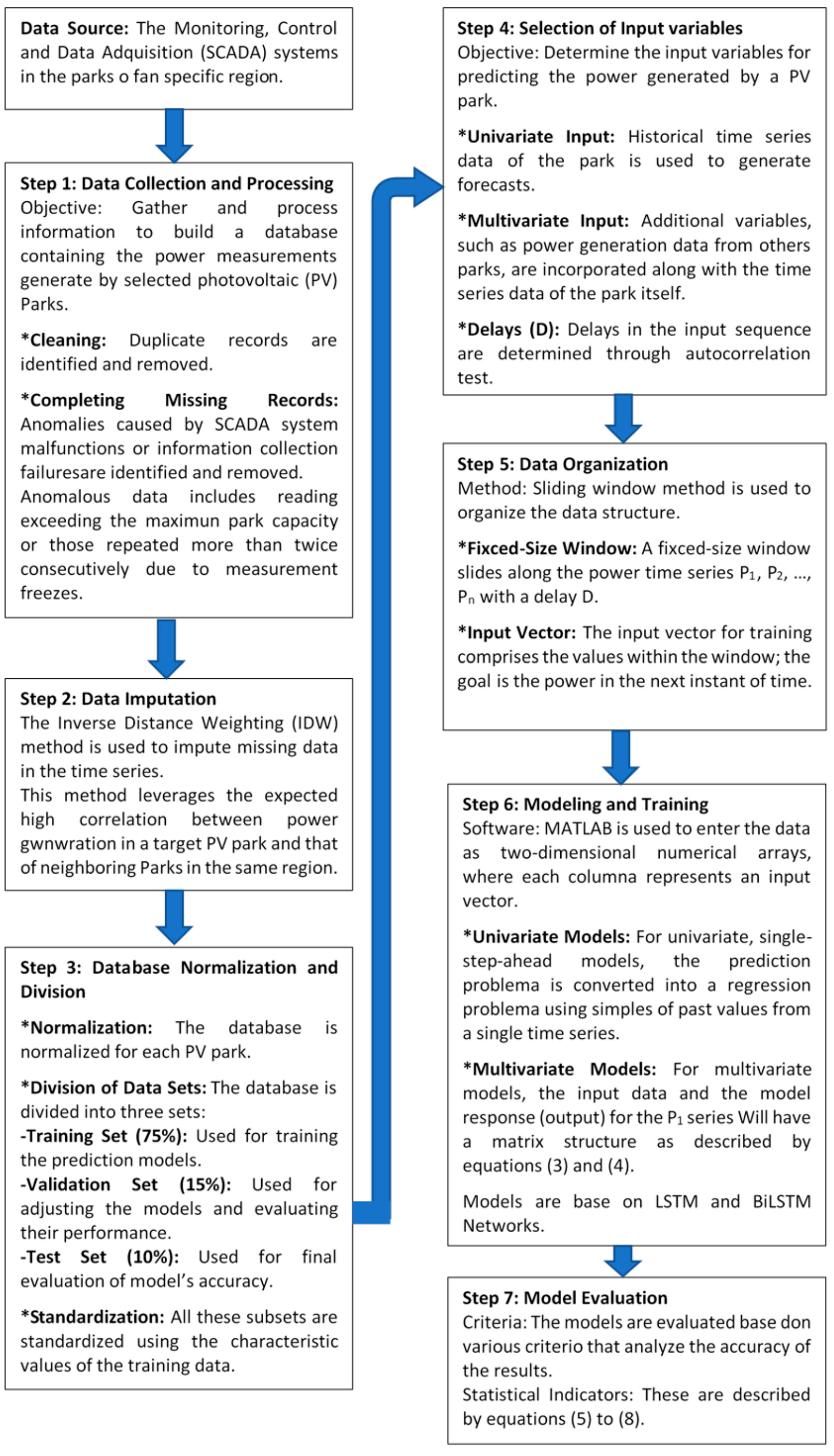
Figure 1 describes the general methodology followed to develop forecasting models. The first step is to obtain and process information to build a database containing the power measurements generated by the selected PV parks. The monitoring, control, and data acquisition (SCADA) systems in the photovoltaic parks of a specific region provided this information.
For data processing, researchers designed software to automate the cleaning and completion of the database imported from Excel spreadsheets, and to identify and remove duplicate records during the process and complete missing records. SCADA system failures or information collection issues can lead to data anomalies. These anomalies include readings that exceed the maximum park capacity or values repeated more than twice consecutively because of measurement freezes. To address these issues, we implemented a two-step process to handle outliers and missing data. First, we identified outliers using the MATLAB Statistics Toolbox to detect outliers in the data. The approach adopted was based on the mean and standard deviation, setting a threshold of three times the standard deviation to ensure that only extremely improbable values were flagged as outliers.
Second, to correct both identified outliers and actual missing data, we applied the inverse distance weighting (IDW) method. This approach leverages the high spatial correlation between energy generation in neighboring parks within the same geographic region. A previous work validated the correlation between parks using a Pearson correlation coefficient analysis, yielding average values exceeding 0.85 in all cases. The IDW method assigns greater weight to data from parks closer to the point of interest, gradually decreasing the weight as the distance increases. In our implementation, we considered a maximum radius of 150 km to select neighboring parks, ensuring that environmental and operational conditions were comparable.
The research used the inverse distance weighting (IDW) method to impute missing data in the time series. IDW is a widely used spatial interpolation technique that estimates missing values based on the weighted average of known values from nearby locations. The weights are inversely proportional to the distance between the target location and the neighboring locations, meaning that closer points have a greater influence on the estimated value than farther ones. This approach is suitable for this study because it leverages the high correlation between energy generation in a target photovoltaic park and that of neighboring parks in the same region [
32]. This method replaces the missing values in the power series of a park with values calculated using Equations (1) and (2).
where
Pi is the power measurement in park i;
W(ri,E) is the weighting function for park i with respect to the estimation park;
ri,E is the distance in kilometers between park i and the estimate park;
n is the number of neighboring parks considered in the interpolation;
p is an interpolation exponent that is generally taken to be equal to two.
After completing and normalizing the database for each PV park, research divided it into a training set (75% of the records), a validation set (15%), and a test set (10%). Before training the forecast models, researchers standardized all these subsets for each park using the characteristic values of the training data. The structure of the predictor variables and the response of the model depend on the prediction horizon and the number of variables and delays considered. It is crucial to determine the input variables to predict the PV power generated by a park, considering not only its availability but also its correlation with the responses [
30].
This research examined two types of models for prediction: univariate and multivariate. Univariate models rely on the historical time series data of the park to generate forecasts. In contrast, multivariate models incorporate additional variables, such as the power generation data from other parks, along with the time series data of the park itself. These models include multiple delays (D) in the input sequence to predict future values, with delays determined through autocorrelation tests. A sliding window method organized the data structure based on [
25]. A fixed-size window slides along the P1, P2, …, Pn power time series with equal size D. The input vector for training comprised the values within the window; the goal was the power in the next instant of time.
This method used Matlab to enter the data as two-dimensional numerical arrays, where each column represents an input vector. For a univariate, single-step-ahead model, for example, the research converted the prediction problem to a regression problem using samples of past values from a single time series under analysis. Thus, the prediction used a univariate regression model with parameters determined through a training process based on historical data up to time t − 1, .
For multivariate models, which consider n time series of power from photovoltaic parks with K records, and for a pre-diction horizon h and delays D, the input data and the model response (output) for the P
1 series will have the following matrix structure described by Equations (3) and (4):
where
P(x) is the power of park x;
D is the number of delays that will be used for the prediction;
h is the prediction horizon.
2.1. Model Quality Statistics
A meticulous evaluation, based on various criteria that analyzed the accuracy and adequacy of the results, determine the final prediction model. Among the statistical indicators commonly used to evaluate the performance of prediction models are the mean absolute error percentage (MAPE), mean absolute error (MAE), root-mean-square error (RMSE), and correlation coefficient (r). The calculation of these indicators is as follows:
where N is the number of observations, P(t) is the measurement of the power generated in t,
is the prediction of the power generated in t,
is the average value of the power generated and
is the average value of the forecasted power.
2.2. Architecture and Operation of Neural Networks Used in Modeling
The LSTM (long short-term memory) and BiLSTM (bidirectional LSTM) neural networks, specialized architectures within recurrent neural networks (RNNs), handle and learn patterns in data sequences, such as time series, text, and signals.
2.3. LSTM (Long Short-Term Memory)
Hochreiter and Schmidhuber proposed LSTMs in 1997 to overcome the limitations of traditional RNNs, which have difficulty handling gradients and remembering information in the long term because of the problem of gradient fading or bursting. LSTMs address this problem by using memory units called memory cells, which have an internal structure that allows information to be maintained and updated for long periods of time.
2.4. Architecture and Operation of LSTM Networks
A long short-term memory (LSTM) network is a recurrent neural network architecture designed to capture long-term dependencies in data streams. The architecture of an LSTM comprises several key components that work together to manage information overtime sequences.
Memory cells: Each LSTM unit contains a ct memory cell that maintains the memory state at time t. Specific operations control the flow of information, updating, forgetting, or reading this cell.
LSTM gates: LSTMs use three types of gates to regulate the flow of information within the memory cell:
Forget gate: The forget gate decides what information stored in the memory cell should be forgotten or kept. It is calculated using the sigmoid function , where σ is the sigmoid function, Wf is the weight of the forgetting gate, h(t − 1) is the hidden state in the previous time, x(t) is the current input, and bf is the bias of the forgetting gate. The result f(t) is a vector of values between 0 and 1 that indicates how strongly the previous information is forgotten.
Input gate: The gateway determines what new information should be added to the memory cell. It is calculated in two steps: first, a sigmoid function decides which values will be updated: . A tanh activation function then generates an update the candidate vector . The new memory cell c(t) is updated by combining the old value and the new content using: where ⊙ represents element-by-element multiplication.
Output gate: The output gate decides how much of the information in the memory cell should be used as output. It is calculated as follows: where, Wo and bo are the weights and the egress door bias, respectively. The hidden state h(t) is obtained as . This allows only a portion of the current memory cell to be exposed as output, after being modified by the tanh function.
Feedback structure: LSTMs handle long sequences through a feedback structure that allows for the propagation of information through multiple temporal steps. This prevents information degradation as the sequence spreads by connecting the memory cells.
2.5. BiLSTM (Bidirectional LSTM)
BiLSTMs extend unidirectional LSTMs allowing information to flow both forward and backward through the time sequence. This makes them particularly effective at capturing context both ways around each point in the sequence, which is useful in tasks where prediction depends on the past and future history of the data.
2.6. Architecture and Operation of BiLSTM Networks
Two LSTM layers: The BiLSTM comprises two independent LSTM layers for each temporal direction: one that processes the sequence in the temporal order and one that processes it in reverse order.
At each time step, the analysis concatenates the outputs from both LSTMs to form a combined representation of the past and future context.
The BiLSTM grids are useful in tasks where both past and future context need to be considered, such as sentiment analysis, sequence tagging, machine translation, and more recently, in processing time sequences for prediction.
3. Results and Discussion
The aim of this study was to analyze the Yaguaramas photovoltaic park in the province of Cienfuegos, referred to as Parque P1. To enhance the robustness of the analysis, the research include data from the generation of seven additional solar plants in the central region of Cuba. These plants were Caguaguas (P2), Frigorífico (P3), Guasimal (P4), Marrero (P5), Mayajigüa-1 (P6), Mayajigüa-2 (P7), and Venegas (P8). The selected plants spanned 8040 km2 (60 km × 134 km) within the same climatic region.
Researchers calculated Pearson’s correlation coefficient between the Yaguaramas park and the other parks. The results showed a strong positive correlation between the power generated by the parks considered. In particular, the Yaguaramas park exhibited a correlation coefficient greater than 0.85 compared to other parks.
Researchers collected data every 5 min throughout 2021, producing 105,120 energy records per plant, divided into 288 daily intervals. The analysis divided the dataset into training subsets (75%), validation subsets (15%), and test subsets (10%) to ensure appropriate model evaluation.
The first stage comprised verifying the relationship between the power series of the parks to assess whether it was feasible to include data from other parks as predictor variables in the models. Pearson’s correlation coefficient showed a strong positive correlation between the powers generated by the parks, higher than 0.72 with the other parks in Yaguaramas.
Researchers conducted a Granger causality test to assess the inclusion of information from other parks in the forecast models; the test did not reject the alternative hypothesis. In addition, the augmented Dickey–Fuller test verified all series were stationary. The focus of the study was to analyze how the incorporation of data from other parks affected the forecasting models for Yaguaramas park.
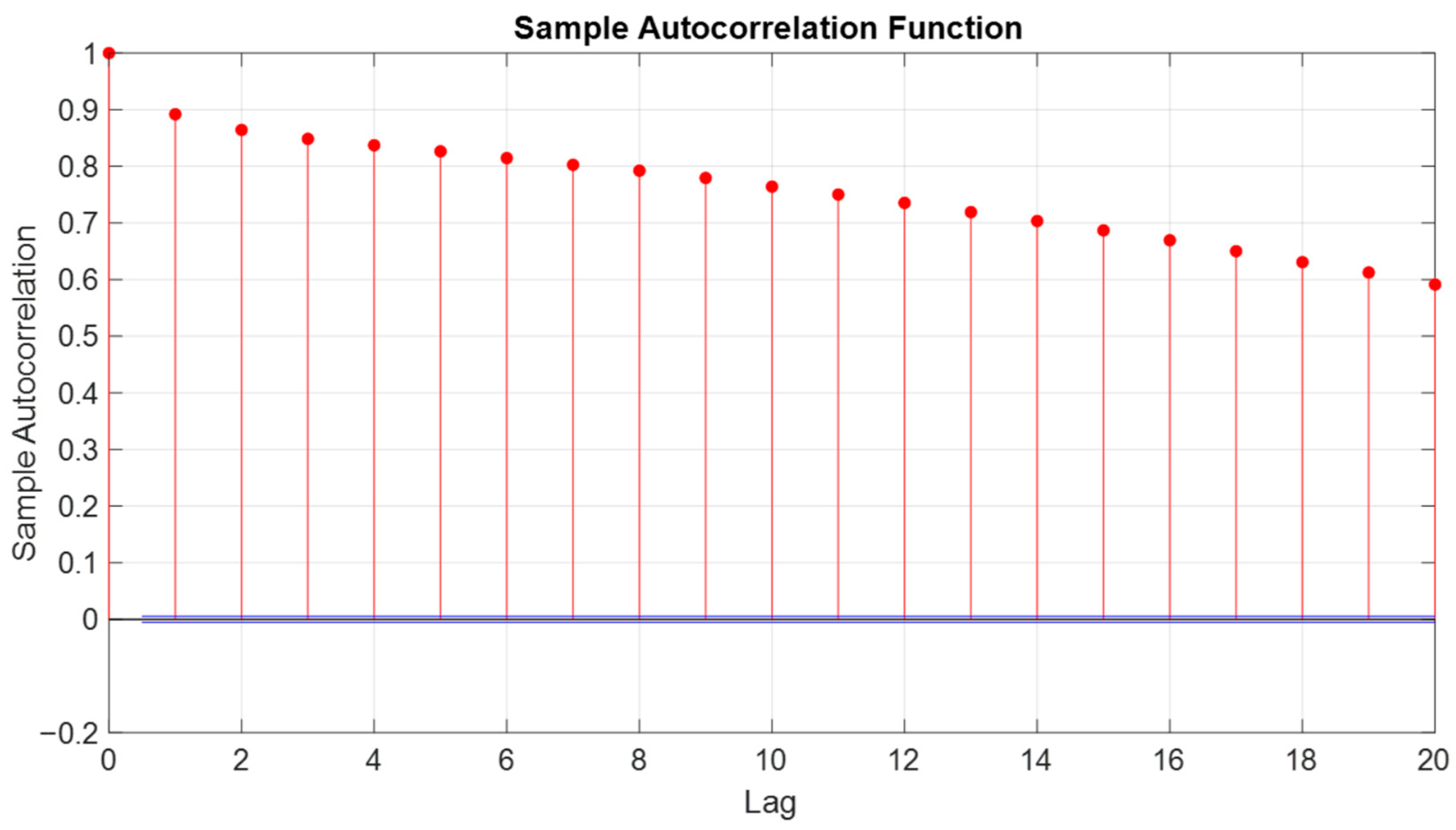
In the study, the autocorrelation function (ACF) was calculated to introduce temporal characteristics into the models.
Figure 2 presents the ACF for the power generated in the Yaguaramas park, together with the 95% confidence intervals (CI). In
Figure 2, the horizontal blue lines are the approximate 95% CI, the vertical red lines are the markers indicating the value of the autocorrelation function of the series with its own lag. The ACF at the zero delay is equal to 1, showing the correlation of a time series with itself, while the horizontal blue lines represent the CIs. The data show a high autocorrelation exceeding 0.8 for up to the first six delays; each delay corresponds to a 5 min interval within the recorded data. The behavior of the all-time series showed an autocorrelation greater than 0.7 up to 10 delays.
The researchers conducted all analyses using MATLAB® R2021b on a portable HP EliteBook 855 G8 laptop equipped with an AMD Ryzen 7 PRO 5850U processor (1901 GHz) and 16 GB of RAM. To optimize the performance of the LSTM and BiLSTM models, a hyperparameter tuning process was carried out. This process involved evaluating multiple configurations of key hyperparameters, including the number of hidden layer units (3 to 153 with a step of 3), validation frequency (250 to 500 with a step of 50), mini-batch size (32, 64, 144, 288, and 432), and early stopping (3, 4, 5, 6, and 7 epochs without improvement). The selection of these configurations was based on their ability to minimize the prediction error metric (RMSE). The final architecture for the best-performing model (Model F) included 128 hidden units, a validation frequency of 500, a mini-batch size of 32, and early stopping after 6 epochs without improvement.
The neural network architecture described processed sequences of data and generated a regression output. The configuration started with a sequenceInputLayer, followed by an LSTM/BiLSTM layer configured to return only the output corresponding to the last time step (OutputMode, last). To regularize the weights and prevent overfitting, L2 regularization factors of 0.1 were applied to both the input weights (InputWeightsL2Factor) and the recurrent weights (RecurrentWeightsL2Factor) and biases (BiasL2Factor). The weight initializers followed the He heuristic (he), which helps speed up training in deep networks, while the bias was initialized using the unit forget gate strategy, commonly used in LSTM/BiLSTM networks to enhance training stability. A dropout layer with a rate of 0.25 followed the LSTM/BiLSTM layer to further reduce overfitting. The network continued with a fully connected layer (fullyConnectedLayer) that reduced the dimensionality to a single output, followed by a regression layer (regressionLayer) that enabled the modeling of continuous prediction problems. This configuration combined advanced regularization and initialization techniques to ensure a balance between modeling capacity and generalization. In univariate models, a single input and output variable is used to predict a future instant within the time series. In contrast, the multivariate models incorporate powers generated in other parks in the region as exogenous variables, besides the series of the target park.
Univariate one-step models use a single variable as input to predict the value of that same variable at a specific future point; this represents the simplest type of prediction. Multivariate one-step models introduce multiple variables to the network to predict a single variable at a single future instant. While the common practice is to use meteorological variables as additional inputs, this research explored the powers generated in other parks in the region, as previously detailed.
The models processed historical records of power generated every 5 min and learned to predict its future behavior. All models developed were for time horizons of 5 min. Because autocorrelation between past and current series values existed, authors investigated models with various time delays to assess their effects on prediction quality. Because of the large number of configurations, this article presents only the models with the best results or that provide meaningful information.
Table 1 details the different cases studied, including their input and architecture.
Models A, B, and C were univariate, using only the power series of the Yaguaramas target park (P1) as inputs. The remaining models were multivariate. The D model included all the series of the parks, including the target park. Models D, E, and F considered only the parks with the highest correlation with the target park, i.e., P1, P2, P4, and P5.
Table 2 shows the statistical indicators to evaluate the quality of the models. These error statistics were the basis for comparison between the different models. The error statistics remained relatively stable and the correlation coefficient r varied between 94.09% and 95.17%, indicating high accuracy in short-term prediction.
3.1. Comparison of the Models
To compare models that operate on the same time horizon, it is necessary to first identify the significant differences between them. To do this, authors used the Tukey test, also known as the Tukey multiple comparisons procedure. This statistical technique is suitable for comparing the means of several groups and determining whether there are significant differences between them. It is useful when making comparisons between three or more groups and seeking to identify which groups differ in relation to a variable of interest. In this study, the Tukey test allowed us to compare the error or residual between the forecasts generated by the models and the actual power measurements. The test implementation used Matlab’s multcompare function. Interpretation of the Tukey test results was based on the confidence interval for the difference between the two means. If this interval did not include zero and the associated p-value was less than the significance level (α = 0.05), results concluded that a significant difference existed between the models in terms of prediction error.
The A, B, and C models were univariate and had significant differences from each other, as shown by Tukey’s test. When evaluating the performance of these models using error metrics (RMSE, MAE, and MAPE) and correlation coefficient (r), Model C stood out as the best among univariate models with a 5 min horizon. Although the ASM of Model C (107.56%) was higher than that of the other models, its RMSE (407.24 kW) and MAE (138.80 kW) values were lower, and its correlation coefficient (95.08%) was slightly higher, showing a better fit.
Among the multivariate models with a 5 min horizon, comparison of Models D, E, and F showed Model F had the lowest RMSE (400.63 kW). Although its MAE (147.66 kW) was slightly higher than that of Model E (141.96 kW), it was lower than that of Model D (162.44 kW), and its correlation coefficient was comparable. Authors preferred Model F because of its lower complexity; it used only two input variables, thus reducing data preparation, computational cost, and training time.
For 5 min time horizons, Models C (univariate) and F (multivariate) were the standouts, both based on BiLSTM networks and incorporating six delays from each time series into the input characteristics. According to
Table 2, Model F showed a slightly lower RMSE (400.63 kW) and ASM (102.03 kW) than Model C (407.24 kW and 107.56 kW, respectively), showing higher accuracy. In addition, the correlation coefficient of Model F (95.17%) was slightly higher than that of Model C (95.08%), which reinforced its better adjustability.
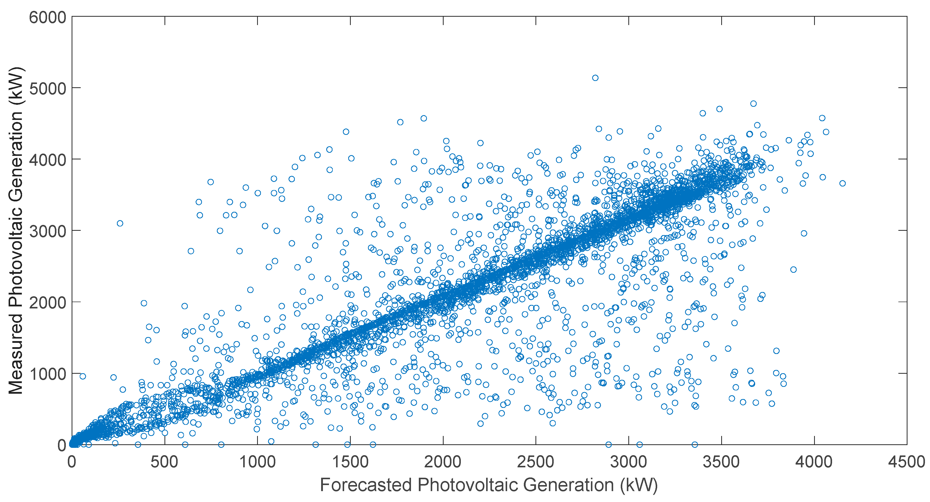
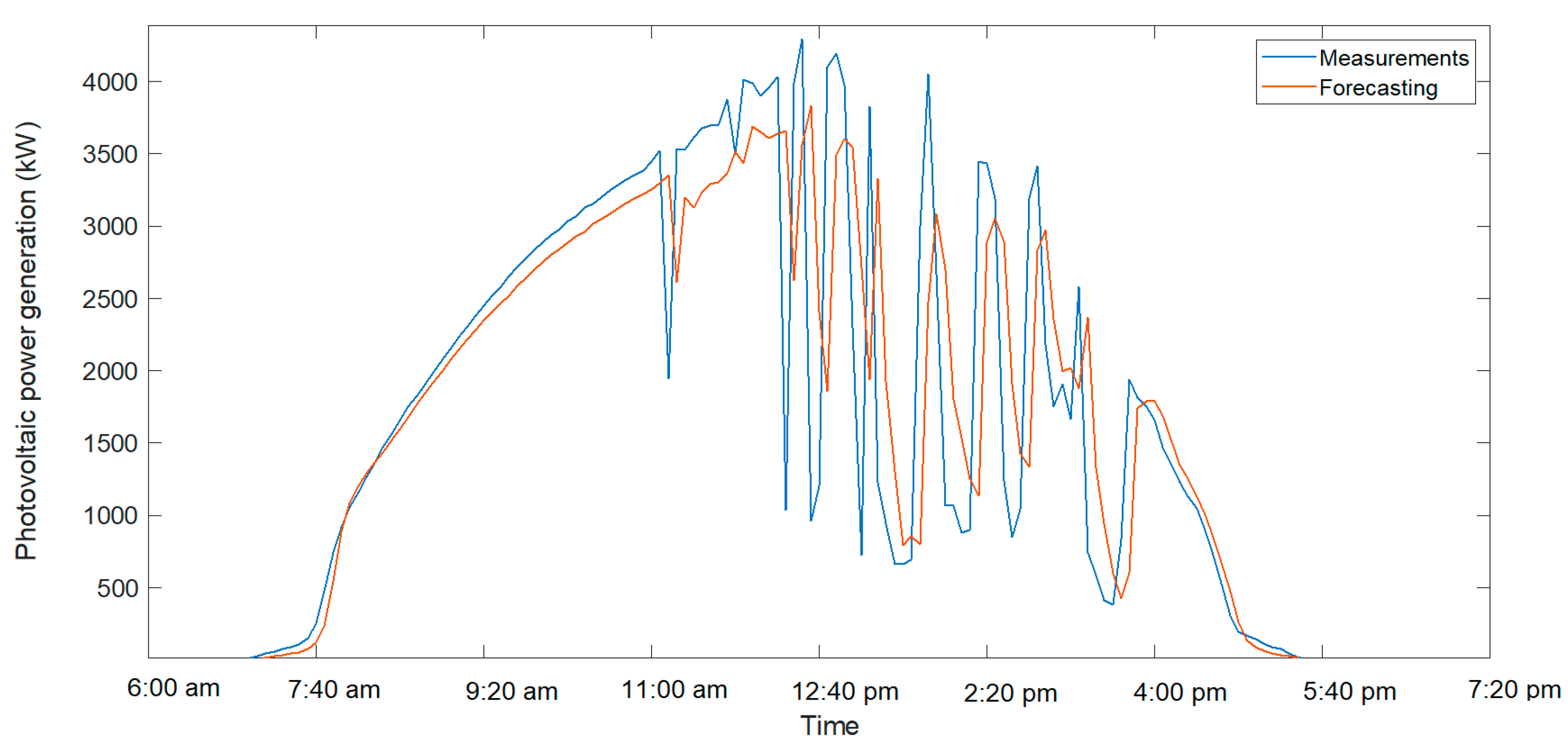
Figure 3 illustrates the correlation between the measured and predicted power values using Model F for the test dataset. The data represent a 5 min time horizon, with predictions generated for both clear and cloudy days. Cloudless days exhibited more uniform power generation patterns because of constant solar irradiance, while cloudy days showed abrupt fluctuations caused by intermittent cloud cover. The high correlation coefficient (r = 95.17%) showed that Model F effectively captured these variations, demonstrating its capability to adapt to different weather.
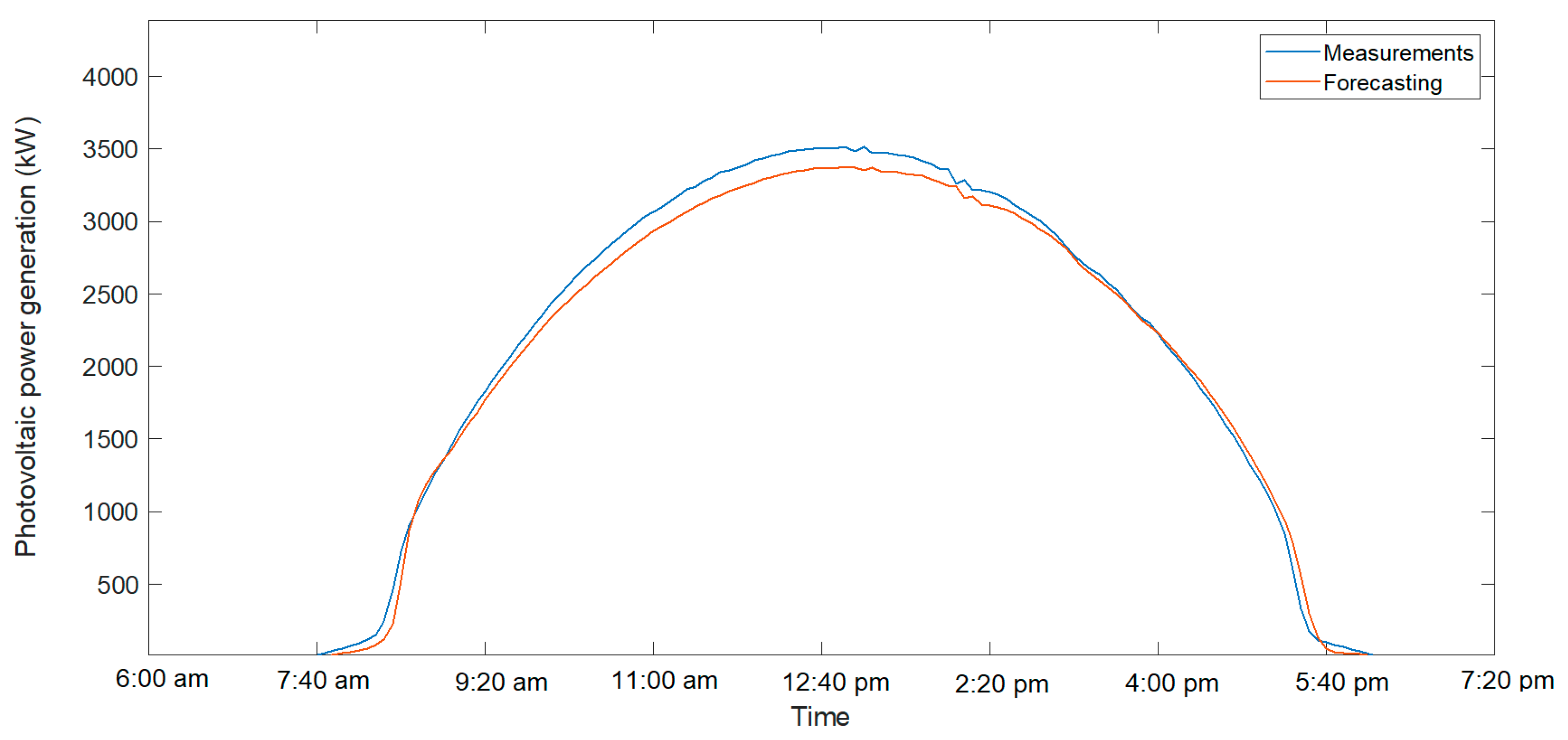
Figure 4 and
Figure 5 show the forecast results and the actual value for a cloudy day and a clear day, respectively. In these graphs, for clear days, the prediction was better adjusted to reality, while for a cloudy day, with sudden variations in generation, the result was slightly worse.
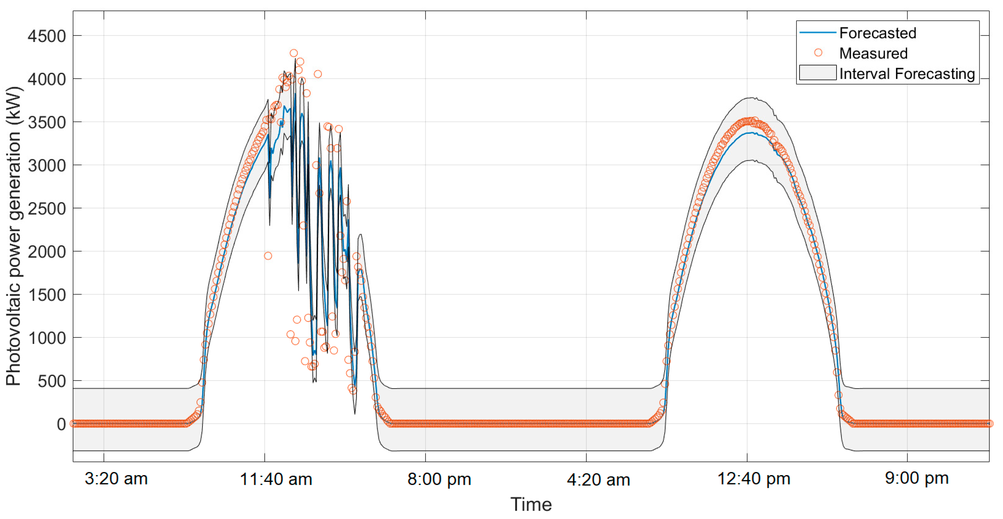
3.2. Forecast Interval
Predicting with confidence interval rather than simply providing a point value is critical to more informed and effective decision-making. A confidence interval not only provides an estimate of future value but also reflects the uncertainty and variability inherent in predictions. This is especially important in contexts such as PV generation, where factors such as weather can cause significant fluctuations. A confidence interval allows managers to plan and prepare for different scenarios, rather than relying solely on an estimate that might prove inaccurate. In addition, it provides a more robust measure of risk associated with decisions, helping to optimize resources, reduce the impact of errors, and improve the reliability of operational and control strategies.
Quantile regression is a useful technique for managing uncertainty in PV power forecasts. Rather than just estimating an average value, this method allows you to obtain confidence intervals that show how the forecast varies in different parts of the error distribution. To use quantile regression, the first step is to calculate the differences between the actual and predicted values, creating a set of errors. Then, we estimate certain percentiles of these errors—for example, the 5th (0.05 quantile) and the 95th (0.95 quantile)—using MATLAB’s quantile function.
Researchers added or subtracted these percentiles from the original predictions to obtain a range of potential future values. This range, or forecast interval, showed where future observations were likely to fall, considering variability in errors. For example, when applying this method to Model F to predict power over a 5 min horizon, it was observed that, for a cloudy day with significant fluctuations in energy generation, most of the values fell within the prediction range. For sunny days, all values were adjusted to this range. Thus, quantile regression offered a more comprehensive way to assess and manage uncertainty in our forecasts, helping to make more informed decisions and assess risks more effectively.
Figure 6 shows the confidence interval.
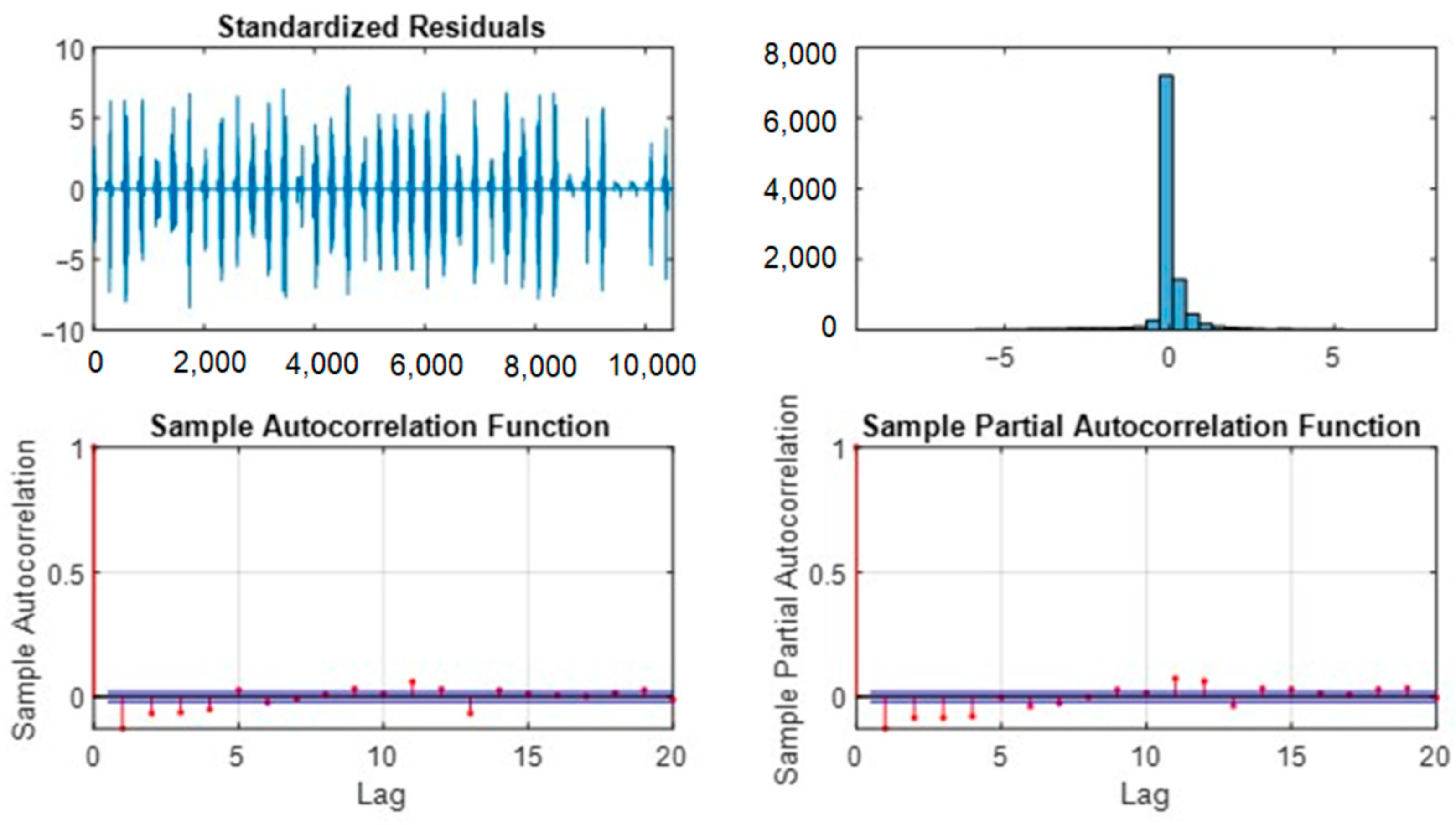
3.3. Residual Analysis of the Model
Figure 7 shows the analysis of Model F residuals, showing positive model fit results. The absence of residual autocorrelation shows the model was not omitting important temporal patterns in the data, suggesting that Model F was well-specified and effective in predicting. Although the histogram of residues was not perfectly normal, it resembled a normal distribution, which is a good sign, although not ideal.
This suggests that Model F provided accurate predictions overall, but there are areas where the model could improve. To improve future results, authors suggest data transformations or alternative models to improve residual normality. They also recommend investigating and handling outliers and adjusting hyperparameters. These actions could help optimize the accuracy and robustness of the model in future analyses.
4. Comparison with Previous Models and Contributions
This study introduces an innovative approach for very short-term forecasting of photovoltaic (PV) energy, using multivariate models that incorporate non-climatic exogenous variables. The major innovation lies in using time-series data from neighboring PV plants as inputs, rather than relying solely on meteorological data or univariate models. This strategy addresses an important gap in the literature, as highlighted in [
2], where the integration of spatial correlations between plants has been explored rarely.
The authors investigated the development of several models for the case study park [
9,
12], combining the discrete wavelet transform (DWT) model with artificial neural networks (feed-forward backpropagation and generalized regression neural networks) to decompose and reconstruct the time series of power and meteorological variables. Although these models achieved excellent results, their dependence on meteorological data and a more complex structure limited their precision. For example, the hybrid model in [
9] presented a MAPE of 33.89%, an RMSE of 1.5 MW, and an error variance (σ
2) of 0.32. In contrast, the models proposed in this article introduce significant simplification and improvement by employing long short-term memory (LSTM) and bidirectional LSTM (BiLSTM) neural networks, which integrate power data from other plants in the region as predictive variables. This innovation allowed for greater accuracy, with Models D, E, and F exhibiting RMSE values between 400.63 kW and 404.29 kW, MAPE values between 94.12% and 102.03%, and a correlation coefficient (r) between 95.08% and 95.17%. Specifically, Model F stood out for its reduced complexity (only two inputs) and superior accuracy metrics, with an RMSE of 400.63 kW, a MAPE of 102.03%, and a correlation coefficient of 95.17%, demonstrating a notable improvement compared to previous models.
To better understand the advantages of the proposed method, we conducted a comparative analysis between univariate and multivariate models. Univariate models, such as Models A, B, and C, are based only on historical energy data from the target plant (P1). While these models provide reasonable accuracy, they cannot capture broader spatial patterns and correlations present in the regional energy generation dynamics. For instance, Model C, the best-performing univariate model, achieved an RMSE of 407.24 kW and a correlation coefficient of 95.08%. However, the lack of external inputs explaining variability beyond the target plant’s immediate environment limited its performance.
In contrast, multivariate models, such as Models D, E, and F, incorporate power series from highly correlated neighboring PV plants. These models showed superior predictive capabilities, particularly Model F, which achieved the lowest RMSE (400.63 kW) and the highest correlation coefficient (95.17%). Including exogenous variables allowed Model F to more effectively capture spatial dependencies and temporal patterns, leading to more accurate and reliable predictions.
A key advantage of the proposed method is its robustness in handling scenarios with limited meteorological data. Traditional forecasting methods often heavily rely on weather forecasts or numerical weather prediction (NWP) models, which may not always be available or accurate. By focusing on power series data from neighboring plants, our method provides a practical solution for regions where meteorological information is scarce or unreliable.
The study highlights the importance of model selection and architecture design. Using BiLSTM networks in multivariate models (e.g., Model F) demonstrates their ability to capture bidirectional temporal dependencies, which are crucial for understanding past and future trends in PV energy generation. This contrasts with LSTM-based models, which process information only in one forward direction and may overlook important contextual relationships.
To underscore the impact of the proposed method,
Table 2 compares the performance metrics of univariate and multivariate models. The results clearly show that incorporating exogenous variables significantly improved prediction accuracy. For example, Model F reduced the RMSE by approximately 6.61 kW compared to Model C while maintaining a comparable MAE and achieving a slightly higher correlation coefficient. These improvements highlight the value of integrating spatial correlations into forecasting models.
Last, the application of quantile regression to calculate confidence intervals further enhanced the practical utility of the proposed method. By providing solid estimates of uncertainty, this technique enables grid operators to make informed decisions and prepare for various scenarios, especially during periods of high variability, such as cloudy days.
5. Conclusions
This study evaluated the efficacy of advanced multivariate models for the very short-term prediction of PV power generation, integrating data from power series from multiple plants as exogenous variables.
Incorporating power series data from nearby PV plants as exogenous variables in the prediction models has proven to be effective in improving the accuracy of 5 min estimates. Multivariate models that include data from multiple PV parks show superior performance compared to univariate models based solely on data from the target farm.
Among the models evaluated, Model F, which used BiLSTM networks and data generated from power in parks with high correlation with the target park, showed the best overall performance. This model had the lowest mean square error (RMSE) and a higher correlation coefficient, showing a greater ability to adjust predictions to real values.
Including power data from other PV parks not only improves the accuracy of predictions but allows them to capture spatial patterns and correlations that are not reflected in univariate models. This approach allows for better management of variability in power generation, facilitating a more effective integration of solar energy into the electricity grid.
The application of quantile regression to calculate confidence intervals has proven to be useful in managing uncertainty in predictions. Confidence intervals provide a more robust measure of variability and help plan and prepare for different scenarios in power generation.
The results of this study have significant implications for the planning and operation of photovoltaic systems. The ability to forecast generation with high accuracy and consider the associated uncertainty facilitates better management of the power grid, optimization of resources, and reduction of operating costs. Implementing advanced multivariate models can significantly improve the integration of renewable energies and the stability of electricity systems.
Future research could focus on optimizing hyperparameters, handling potential outliers, and applying transformations to the data to further improve the accuracy and robustness of the model.


 ,
, 
