Grid-Forming: A Control Approach to Go Further Offshore?

Abstract

Offshore wind farms are increasingly being commissioned farther from shore, and high voltage alternating current (HVAC) transmission systems are preferred because of their maturity and reliability. However, as cable length increases, ensuring system stability becomes more challenging, making it essential to investigate shunt reactor compensation configurations and converter control strategies. This study examines three different shunt reactor compensation arrangements and two control strategies, grid-forming (GFM) and grid-following (GFL), across three cable lengths (80 km, 120 km, and 150 km). The systems were evaluated based on small-signal stability using disk margins for different active power operating points, and later for different short-circuit ratios (SCR) and X/R. The results demonstrate that the GFM is preferable for longer cables and enhanced stability. The most robust configuration includes a shunt reactor placed in the mid-cable with additional reactors at both ends of the cable, followed by an arrangement with reactors at the beginning and end. The GFM converter control maintained stability across all operating points, cable lengths, and configurations, whereas the stability of the GFL unit was highly dependent on active power injection and struggled under weaker grid conditions. Thus, for longer HVAC cables, it is necessary to employ GFM control units, and it is recommended to use shunt reactors at the cable start and end, as well as at mid-cable, for optimal stability.

1. Introduction

The established targets in the Paris Agreement to meet net zero emissions has led to the replacement of fossil fuel synchronous-based generators by inverter-based renewable energy sources (RESs). Offshore wind power plants (OWPPs) are one of the most secure, cheap, clean, and reliable RESs [1]. The installed capacity of OWPPs in Europe is currently 28 GW. More than 12 GW come from the United Kingdom, which installed 2.6 GW in 2021 [2], and it is expected to exceed 40 GW by 2030.

With the intention of harnessing steadier and stronger winds, OWPPs are being commissioned further away from the shore. This increase in distance leads to the need for longer High Voltage Alternate Current (HVAC) submarine export cables or even a switch to High Voltage Direct Current (HVDC) connections. HVAC connections are preferred due to their maturity and reliability. However, as the distance from the OWPPs to the onshore transmission system increases, it is suggested that HVDC connections become cost competitive [3], with a break-even distance that is considered to be between 80 and 100 km [4,5,6].

1.1. Literature Survey

Several considerations are being given to ways in which HVAC technology can be used for longer, yet reliable, and robust export cables [3,7,8,9,10,11]. HVAC-XLPE cables have a high inherent capacitance, which is dependent on cable length, insulation, and construction materials. This capacitance causes a leading power factor, and therefore a leading reactive power. To maintain the power quality and voltage stability of the system, the reactive power needs to be balanced, which is achieved using shunt-connected reactive power compensation devices. With the addition of lagging reactive power components in the system, the power factor can be adjusted closer to unity, reducing losses and enhancing transmission efficiency and stability [12,13].

Several projects involving long HVAC export cables with shunt reactive compensation have already been commissioned. An inter-connector was installed between Malta and Sicily with a voltage of 245 kV, an overall cable length of 117.6 km, and two asymmetrical shunt reactor compensations at both ends of the cable [14,15]. The East Anglia 1 OWPP commissioned a 420 kV, 100 km HVAC export cable which exports 714 MW [10]. The West of Adlergrund involves a 90 km long HVAC export cable with a nominal voltage of 245 kV, exporting 250 MW [16].

Shunt compensation close to the connection point between the sea and land cables was installed in the Horns Rev B OWPP, which exports 210 MW of power at a nominal voltage of 150 kV. In [17], it was observed that commissioned shunt compensation led to a reduction in the cable loading and a reduction in yearly losses of 23%. Furthermore, the voltage was maintained between the acceptable limits established by the Danish transmission system operator (TSO). The overall cable length was slightly greater than 100. However, the undersea export cable was only 42 km.

A multi-objective optimization function was utilized in [18] to determine the optimal location and value for shunt reactive compensation. This was performed by considering the reduction in power losses, minimization of the cost of such compensation and improvement in the voltage profile. It was observed from the study that the employment of these devices depends on the voltage level of the overall system and the cable length. For lower voltages and shorter distances, two reactors would suffice; however, for longer distances, the configuration with three reactors provides lower losses and cost.

1.2. Motivations

Following the previous study described, Dakic et al. compared HVAC transmission with shunt compensations, varying its location, and VSC-HVDC technology [19]. It was concluded that the most cost-effective transmission system was the HVAC topology with three shunt reactors, including an offshore mid-cable reactor. This solution is said to be valid for high OWPPrated power and cable lengths ranging between 70 km and 150 km. It was also concluded that 220 kV was the most favorable option from all the voltages analyzed. Following this analysis, the aim of the present study is to analyze the stability of the options described in [19], with OWPPs connected via long HVAC export cables, focusing on the performance of two converter control modes: GFM and GFL. While both control modes are analyzed, particular emphasis is placed on GFM due to its potential to overcome the challenges of long-distance HVAC transmission and weak grid conditions, areas where GFL is known to face limitations. The research questions focus primarily on GFM because it represents a promising technology for extending HVAC cable lengths and improving stability, yet its performance in such configurations remains underexplored. This study aims to bridge this gap by investigating whether GFM can enhance the stability and robustness of the overall system compared to the established GFL approach.

Currently, most grid-tied inverters operate via GFL control, which controls the current injected by the converter with a phase displacement from the grid voltage at the point of common coupling (PCC). However, GFM does not require prior knowledge of the system frequency because both the magnitude and phase of the voltage are controlled [20,21]. GFM controllers also enhance grid resilience and enable the wind farm to operate autonomously, in island mode, or even supply power to local loads in the absence of a stable onshore electrical grid, which may be advantageous during grid disturbances or in a black start scenario [22].

Research shows that from an academic point of view concerning VSC technology, GFM controllers are preferred because of their increased stability, enhanced resilience, and improved grid integration for RESs [20,23,24,25,26]. However, there is a gap in academia regarding the use of an OWPP with GFM capability connected to long HVAC transmission systems that require shunt reactive compensation.

Therefore, this study answers the following questions:

• Can the length of an HVAC export cable be extended by employing a GFM controller?
• Is the stability and robustness of the overall system enhanced with a GFM controller?
• What system arrangement (i.e., location of shunt compensation) enhances the stability?

To address these questions, this study compared three different arrangements, each varying the location of shunt compensation. Additionally, three cable lengths—80 km, 120 km, and 150 km—were assessed. The study compared GFM and GFL controllers using a small-signal model, considering various active power injections from 0 pu to 1 pu. The stability was analyzed using disk margins to evaluate the robustness of each configuration. Furthermore, the stability of the system was analyzed for a lower short-circuit ratio (SCR) and different levels of X/R, as to test the system against weaker networks.

The remainder of the paper is organized as follows. Section 2 outlines the system configurations that were defined for the study. Section 3 introduces both control strategies, detailing their implementation and differences. Section 4 presents the stability analysis, beginning with an explanation of the system linearization process, followed by the validation of the small-signal model against the EMT model, and concluding with the stability assessment. Section 5 conducts an analysis similar to that of Section 4, but focuses on a parameter sweep for the SCR and X/R, to analyze the impact of control strategies and system arrangements on weaker grids.

2. System Configurations

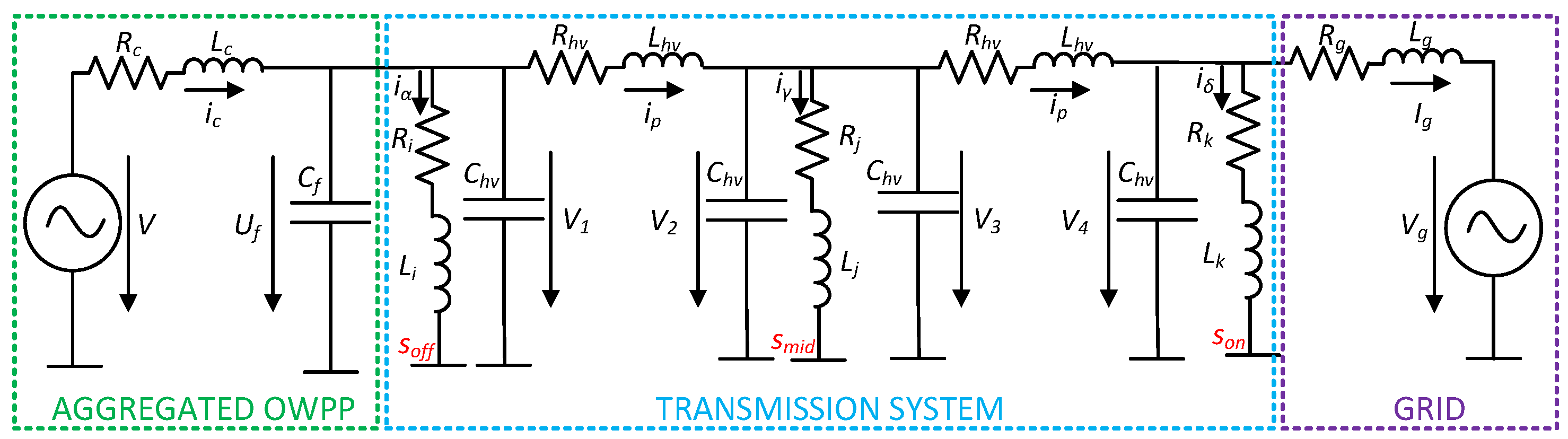
The system under consideration is illustrated in Figure 1. It can be observed that it features two arrows: one pointing to the left, indicating the offshore side, and the other pointing to the right, representing the onshore network. It consists of an OWPP connected to a transformer that steps up the voltage to 230 kV. The transmission system includes an HVAC submarine cable and shunt reactive power compensation components distributed along the line. These shunt components are varied across the different configurations studied in this work. The system is then connected to an onshore local network. For this specific study, an aggregated wind farm model is used, encapsulating both the OWPP and the offshore transformer.

The detailed modelling approach for the system is shown in Figure 2. The aggregated OWPP is represented as a voltage source with voltage V and an L_C filter characterized by parameters $R_c$ and $L_c$. This impedance accounts for the contribution of the park transformer. The transmission system comprises an HVAC submarine cable with shunt reactive power compensation components, which manage the capacitive reactive power of the long cable. These shunt components are further explained in Appendix A. The electrical grid is represented by a Thevenin equivalent, defined by voltage $V_g$, resistance $R_g$, and inductance $L_g$. This model is used to analyse the stability and performance of the system under various operational scenarios.

The export cable was modeled using a $\pi$-equivalent circuit with parameters $R_{hv}$, $L_{hv}$, and $C_{hv}$. For simplicity and because this study focuses on small-signal analysis, the shunt compensations are modeled as reactors, with their values calculated based on the amount of reactive power to be compensated. The parameters used in this study may be seen in

Table A2. System parameters.

Parameter	Value	Unit
$S_{base}$	350	MVA
$U_n$	230	kV
$SCR$	1.5/3	-
$X/R$	1.5/5/10	-
$L_g$	0.096	H
$R_g$	0.302	Ω
$L_c$	0.048	H
$R_c$	1.511	Ω
$C_f$	3.160	μF
$R_{hv}$	0.2620	Ω/km
$L_{hv}$	0.0018	H/km
$C_{hv}$	0.11	μF/km

of Appendix B.

Several hardware arrangements for export cables with shunt compensation were examined, focusing on the different numbers and locations of the shunt reactors. This section describes how these setups affect the voltage profiles for various cable lengths as well as the power factor. The shunt compensation can be placed in three locations: at the sending end of the cable immediate after the OWPP ($s_{off}$), in the middle of the cable ($s_{mid}$), or at the receiving end, onshore ($s_{on}$).

Three different arrangements were identified, as listed in

Table 1. Arrangements of shunt compensation analyzed.

Arrangement	Location Reactors
A1	$s_{off}$ + $s_{on}$
A2	$s_{off}$ + $s_{mid}$ + $s_{on}$
A3	$s_{on}$

. In arrangement A1, shunt compensations are placed at both the offshore PCC and onshore PCC. Arrangement A2 involved shunt reactors located offshore, mid-cable, and onshore. In arrangement A3, a single shunt reactor was positioned onshore. The shunt reactors were sized as described in Appendix A and their final values for the different arrangements, A1, A2 and A3, and for the different cable lengths are shown in

Table A1. Reactive power measured and shunt reactors values in (H) for the three cable lengths, for SCR = 3 and X/R = 5.

	Cable Length (km)
	80	120	150
Q (MVAr)	138	210	240
A1 (H)	0.49 + 0.73	0.32 + 0.48	0.28 + 0.42
A2 (H)	2.53 + 2.43 + 3.37	1.26 + 1.26 + 1.68	0.84 + 0.84 + 1.22
A3 (H)	0.48	0.43	0.16

.

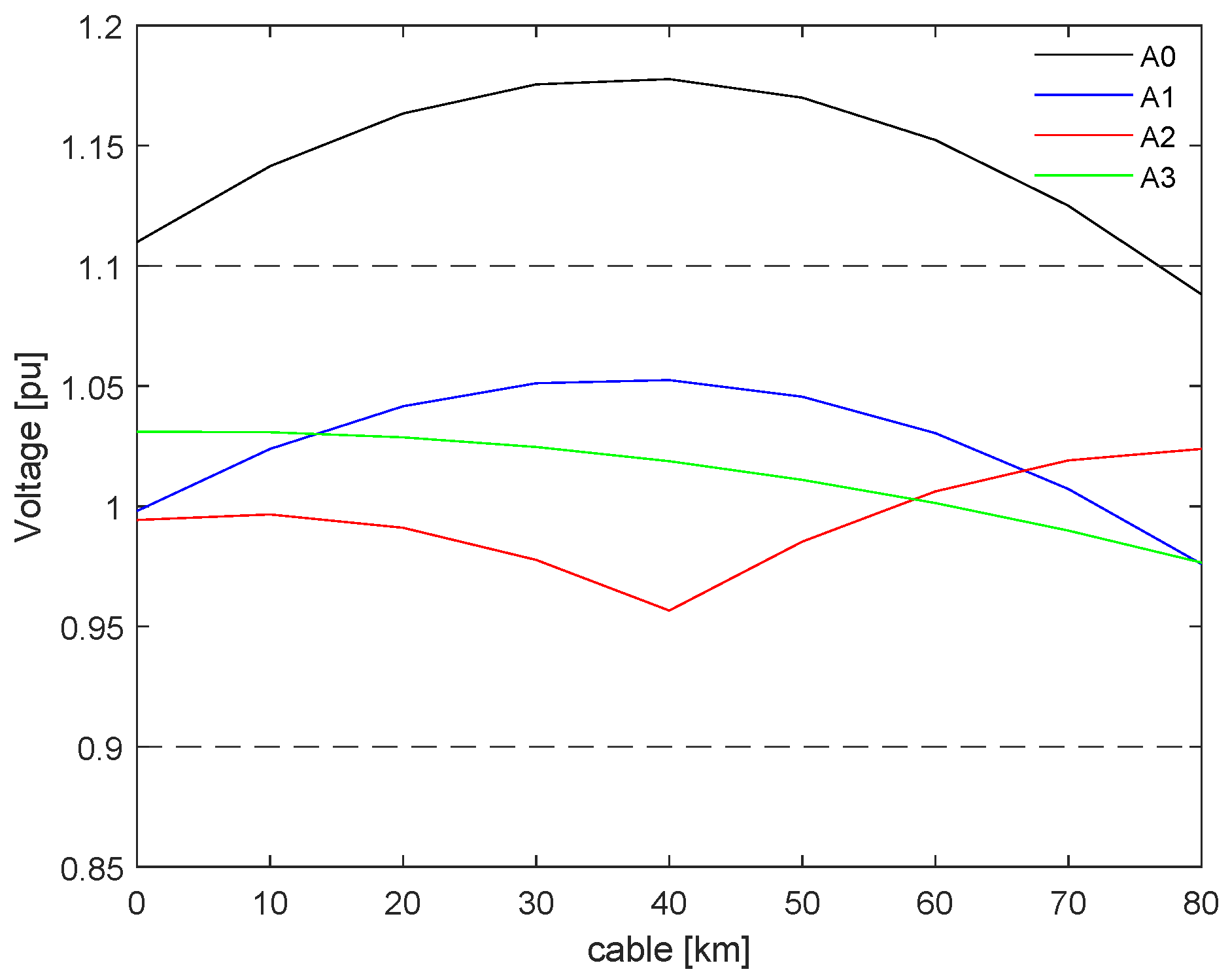
Shunt reactors were installed to comply with the standard requirements set by most TSO. The main objective was to maintain the voltage within acceptable limits, specifically between 0.9 pu and 1.1 pu, and to ensure that the power factor remained within the range of −0.95 to 0.95, lagging at the point of common coupling (PCC). The voltage profile results for an 80 km export cable, considering the various compensation arrangements, are shown in Figure 3. In this Figure, “A0” represents a scenario without shunt compensation. Voltage measurements were taken at the sending and receiving ends of the cable, as well as at 10 km intervals along its length. The results indicate that, without appropriate reactive power compensation, the voltage exceeds the specified TSO limits. By contrast, the three compensated arrangements, A1, A2, and A3, successfully maintained the voltage within the required limits.

The analysis of shunt reactor placement and sizing revealed that both the location and degree of compensation (as distributed among the reactors) influenced the voltage profile. The corresponding power factor results are presented in

Table 2. Power factor for three cable lengths, and for the case of no compensation (A0) and for the three different arrangements.

	Cable Length (km)
Power Factor	80	120	150
A0	0.7748	0.7071	0.6637
A1	0.9814	0.9752	0.9928
A2	0.9882	0.9973	0.9992
A3	0.9912	0.9873	0.9830

, demonstrating that the implemented shunt compensations maintained both the voltage and power factors within the specified ranges. This analysis was conducted under a SCR of 3, which indicates a weak grid, though not excessively so.

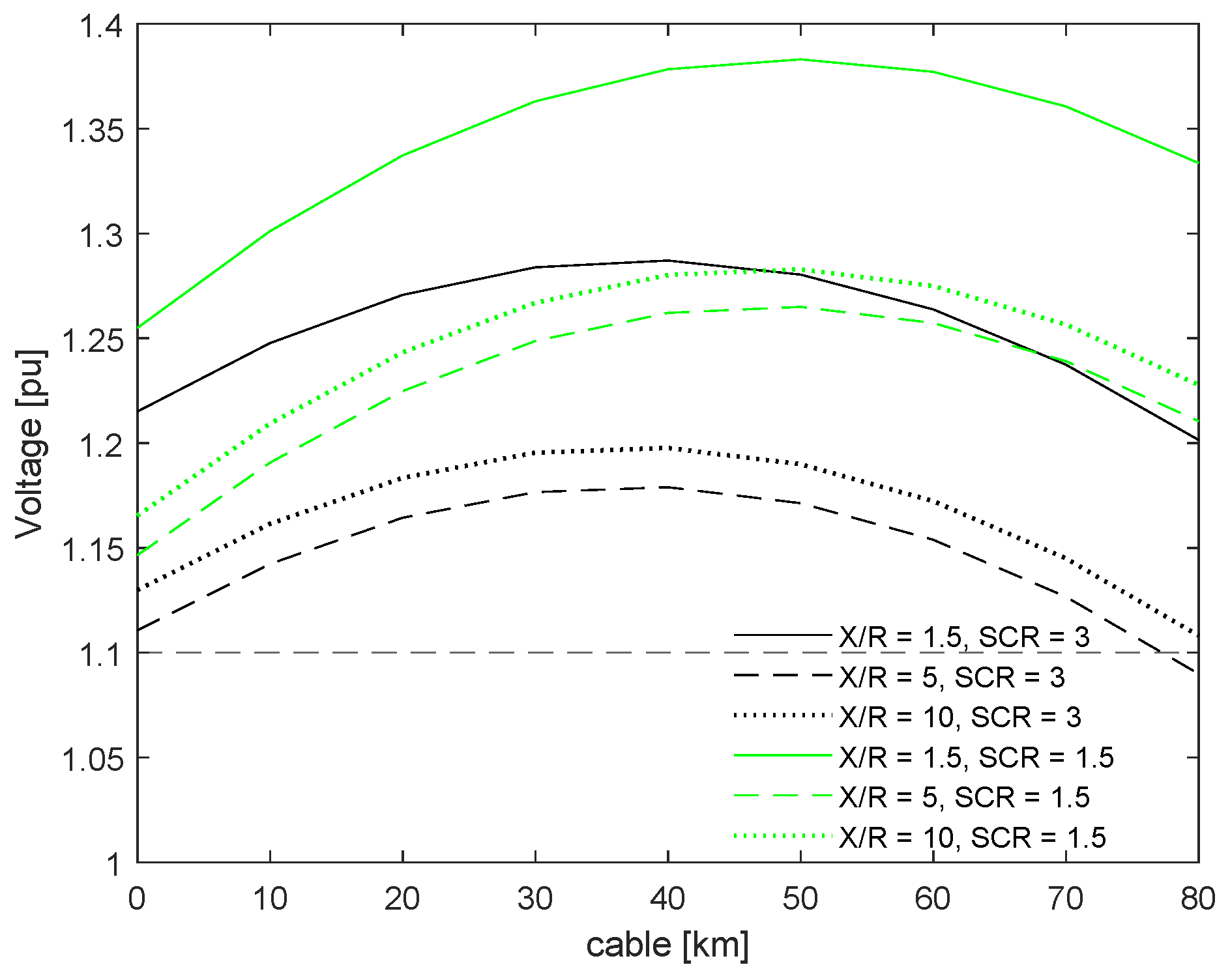
The power factor and voltage profile were also heavily influenced by the strength of the electrical grid, as illustrated in Figure 4. This figure shows an 80 km cable with no shunt compensation under two SCR conditions (1.5 and 3) and for X/R ratios of 1.5, 5, and 10. The results demonstrate that the ability to transfer power and maintain voltage within specified limits is directly related to both SCR and X/R ratios. Consequently, the control and tuning of shunt reactors must be adjusted based on the grid strength. This interdependence means that the overall stability of the power system is closely tied to the strength of the grid: the weaker the grid (indicated by lower SCR and lower X/R ratios), the more shunt compensation is required, which, as will be further discussed in Section 5, will impact system stability.

Changing both X/R and SCR will change the impedance of the overall system, which aligned with the shunt compensations, and the cable length will cause the impedance to vary significantly depending on the arrangement, X/R, SCR, and cable length. This impedance will influence the power factor and voltage profile; hence, shunt reactor compensation will need to be computed accordingly to maintain the PF above 0.95 and a voltage between 0.9 and 1.1 pu.

3. Converter Controllers

This section introduces the GFM and GFL converter controllers used in the study. For Section 4 and Section 5, the tuning process followed the guidelines in [3,27], aiming for an overshoot below 15% and settling time under 500 ms. Tuning was performed at an active power of 1 pu and nominal voltage of 230 kV. The GFM and GFL controller units may be seen sketched in Figure 5 and their parameters used for arrangement A2 with an 80 km cable are detailed in

Table A3. GFM converter parameters for A2, 80 km.

Parameter	Value
$m_p$	1.73 × 10−8
$m_i$	0.91 × 10−7
$k_{p,VCC}$	1.28
$k_{i,VCC}$	22.73
$R_v$	0.38
$L_v$	1 × 10−3

and

Table A4. GFL converter parameters for A2, 80 km.

Parameters	Value
$k_{p,PLL}$	0.0024
$k_{i,PLL}$	0.53
${\tau }_{il}$	2 × 10−3
$k_{p,il}$	1.58
$k_{i,il}$	62.23
$k_{p,PC}$	8.02 × 10−7
$k_{i,PC}$	2.86 × 10−4
$k_{p,QC}$	6.42 × 10−6
$k_{i,QC}$	9.54 × 10−4

, respectively, in Appendix C.

The controller parameters vary with cable length and arrangement due to changes in the overall impedance of the system. The same applies to the SCR and X/R study in Section 5, where new tuning was required since the SCR introduces additional impedance into the grid parameters ($R_g$ and $L_g$).

3.1. Grid Following

The grid-following controller used is the standard vector current controller (SVCC) and a scheme of such may be seen in Figure 5a.

It consists of a $PLL$, a current inner loop, and outer voltage and power loops. The $PLL$ is used to compute the angular velocity of an electrical network. To do so, a PI controller is implemented, as shown in Equation (1):

$$K_{PLL}=k_{p,PLL}+{\displaystyle \frac{k_{i,PLL}}{s}}$$

(1)

where $k_{i,PLL}$ is the integral gain and the proportional term $k_{p,PLL}$. The inner loop represents the lower-level control of the GFL unit. It allows independent control of both q and d components owing to its decoupling terms. The output of this controller is the voltage fed back to the converter. Both components in the synchronous frame are controlled via the PI controller shown in Equation (2):

$$K_{il}=k_{p,il}+{\displaystyle \frac{k_{i,il}}{s}}$$

(2)

where $k_{i,il}$ is the integral gain and the proportional term is $k_{p,il}$. The outer-loop controller computes the current references in the synchronous frame $i_{cq}^{\ast }$ and $i_{cd}^{\ast }$, which are later fed into the inner loop controller. This is achieved by considering the active power and voltage magnitude of the system. Both the voltage and power outer loops are also controlled with PI controllers, as shown in Equations (3) and (4), respectively:

$$K_P=k_{p,PC}+{\displaystyle \frac{k_{i,PC}}{s}}$$

(3)

$$K_V=k_{p,VC}+{\displaystyle \frac{k_{i,VC}}{s}}$$

(4)

where $k_{p,PC}$ and $k_{p,VC}$ are the proportional gains of both the power and voltage outer loop controllers and $k_{i,PC}$ and $k_{i,VC}$ are the integral gains.

3.2. Grid Forming

The GFM unit used in this study belongs to a family of GFM units known as the virtual synchronous machine (VSM). This designation arises from its ability to emulate the behavior of a synchronous machine. A schematic representation of the VSM is provided in Figure 5b, which illustrates a simplified VSM configuration. The controller employed is based on the models described in [28,29], where the outer power PI controller serves as a simplified version of the Swing Equation. In this context, the proportional term corresponds to the damping factor, while the integral term represents inertia. An inner loop current controller was not used, as such controllers are typically employed to manage significant overcurrents, which are not present in this case. This study focuses on small-signal stability, where saturation effects are not represented.

The employed VSM comprises two PI controllers: one is referred to as the power loop and the other is referred to as the voltage loop. The controller includes a virtual impedance.

The power PI loop computes the angle of the PCC. The voltage PI controller computes the $v_q$ component of the voltage to be fed to the converter, where the $v_d$ component is zero. Thus, Clarke transformation is used instead of Park Transformation.

From the figure, the power PI controller $K_{Pm}\left(s\right)$ is defined as shown in Equation (5):

$$K_{Pm}=m_p+{\displaystyle \frac{m_i}{s}}$$

(5)

where $m_p$ is the proportional gain and $m_i$ is the integral gain of the power controller. The voltage loop is defined as follows:

$$K_{Um}=k_{p,VCC}+{\displaystyle \frac{k_{i,VCC}}{s}}$$

(6)

where $k_{p,VCC}$ is the proportional term and $k_{i,VCC}$ the integral term.

Several studies were analyzed with regard to virtual impedance implementation [30,31,32,33,34] and the approach described by Rodriguez-Cabero et al. described in [34] was followed. The virtual impedance is located after the PI voltage loop. Thus, the q component of the voltage fed back to the converter, $v_{lq}$, is given by:

$$v_{lq}=(V_Z^{\ast }-u_{f1,q})\left(k_{p,VCC}+{\displaystyle \frac{k_{i,VCC}}{s}}\right)-i_{c1,q}{R}_v-i_{c1,d}{L}_v\omega$$

(7)

where $V_Z^{\ast }$ is the voltage reference of the controller, $u_{f1,q}$ is the q component of the voltage at the PCC of the GFM converter, and $i_{c1,q}$ and $i_{c1,d}$ are the synchronous reference frame components of the current measured at the converter terminals. For the d component of the voltage at the converter terminals, $v_{ld}$ is given by:

$$v_{ld}=-i_{c1,d}{R}_v+i_{c1,q}{L}_v\omega$$

(8)

In Equations (7) and (8), $R_v$ and $L_v$ are the virtual resistance and inductance, respectively, and $\omega$ is the frequency measured at the PCC.

4. GFM and GFL Controllers Comparison for an HVAC-Connected OWPP

This section focuses on stability analysis, primarily comparing two converter control strategies: GFM and GFL. Additionally, the analysis examines three distinct system configurations, that vary based on the placement of shunt reactor compensations along an HVAC submarine cable. The study also considered three different cable lengths—80 km, 120 km, and 150 km—to evaluate the performance of the converter controllers across various scenarios. The objective is to determine which converter control strategy and system arrangement optimize stability, potentially allowing for longer HVAC cables. Furthermore, the analysis aimed to identify the optimal placement of shunt reactors for enhanced stability.

Given the variability in wind speed and the availability of energy from the OWPP, it was essential to analyze the stability of the different case studies at various operating points. The stability analysis was conducted over a range of power operating conditions. Specifically, the active power was varied from 0 pu to 1 pu in steps of 0.20 pu at nominal voltage.

Small-signal stability was evaluated using disk margins (DM), which quantify the stability and robustness of a closed-loop system by introducing a multiplicative factor f to the open-loop system L, such that $L_s=fL$. While this section provides a brief overview of disk margins, they have been widely employed in numerous studies [28,35,36,37,38].

Two primary approaches exist for DM analysis: the “loop-at-a-time” method and the multi-loop DM analysis. The loop-at-a-time method introduces the perturbation factor f in a single channel (either input or output) while keeping the other channels fixed. Although this method is useful for analyzing individual channel dynamics, it can be overly optimistic, as it does not account for the simultaneous effects of perturbations across multiple channels. To address these limitations, this study applied the more comprehensive multi-loop DM analysis. This approach applies distinct perturbations across multiple channels, represented by a matrix of perturbations F, defined as:

$$F=\left[\begin{array}{cccc}{f}_{1,1}& 0& \cdots & 0\\ 0& f_{2,2}& \cdots & 0\\ ⋮& ⋮& \ddots & ⋮\\ 0& 0& \cdots & f_{n,n}\end{array}\right]$$

(9)

Each element $f_{i,j}$ represents the multiplicative factor applied to the open-loop system L in the channel $(i,j)$. The perturbation factor $f_{i,j}$ is given by:

$$f_{i,j}={\displaystyle \frac{1+\alpha \left(\frac{(1-\sigma )}{2}\right)\delta }{1-\alpha \left(\frac{(1+\sigma )}{2}\right)\delta }}$$

(10)

where $\delta$ is the normalized uncertainty, an arbitrary complex value constrained within the unit disk ($\left|\delta \right|<1$).

The parameter $\alpha$ determines the extent of gain and phase variation modeled by F. For a fixed $\sigma$, $\alpha$ controls the size of the disk of uncertainty. When $\alpha =0$, the perturbation factor $f_{i,j}=1$, meaning the perturbed system is identical to the nominal open-loop system ($L_s=L$). In this case, the Nyquist plot of $L\left(s\right)$ intersects the critical point $-1$, and the system operates at the boundary of stability, with no tolerance for uncertainty. This condition is referred to as marginal stability.

Conversely, larger values of $\alpha$ increase the size of the uncertainty disk, allowing for greater gain and phase variations while maintaining stability. This corresponds to a larger disk margin and enhanced robustness. Thus, for $\alpha >0$, the Nyquist plot of the perturbed system $f_{i,j}L\left(s\right)$ remains clear of the $-1$ point, ensuring stability, while for $\alpha =0$, the Nyquist plot intersects $-1$, resulting in marginal stability, where the system cannot accommodate any perturbations.

In this analysis, the multi-loop input/output disk margin is quantified by a single parameter, $\alpha$, representing the largest disk of perturbations for which the closed-loop system remains stable [30]. Applying factors across all channels simultaneously provides a worst-case scenario for achieving system stability. Therefore, the parameter $\alpha$ was used to assess the stability and robustness of the studied systems. An $\alpha$ value of 0 indicates no tolerance for uncertainty, while values further from 0 indicate greater system stability.

The analysis process involved several steps. First, both GFM and GFL controllers, along with the hardware configurations, were linearized (Section 4.1). These linear, time-invariant models were validated against the EMT models (Section 4.2). The initial conditions were extracted from the EMT model to populate the state-space matrices for all the cable lengths and configurations. Finally, a stability analysis was conducted for all specified active power and voltage operating points, and the results are presented in terms of disk margins in Section 4.3.

4.1. Model Linearization

The nonlinear EMT models were linearized to approximate the system behavior at various active power operating points. This linearization was applied to all the system configurations, including both converter control strategies. Appendix D presents the state-space matrices, $A_{PS}$ and $B_{PS}$, as well as the states $x_{PS}$ and inputs $u_{PS}$ used in the model. The same linearization procedure was applied to the other system arrangements.

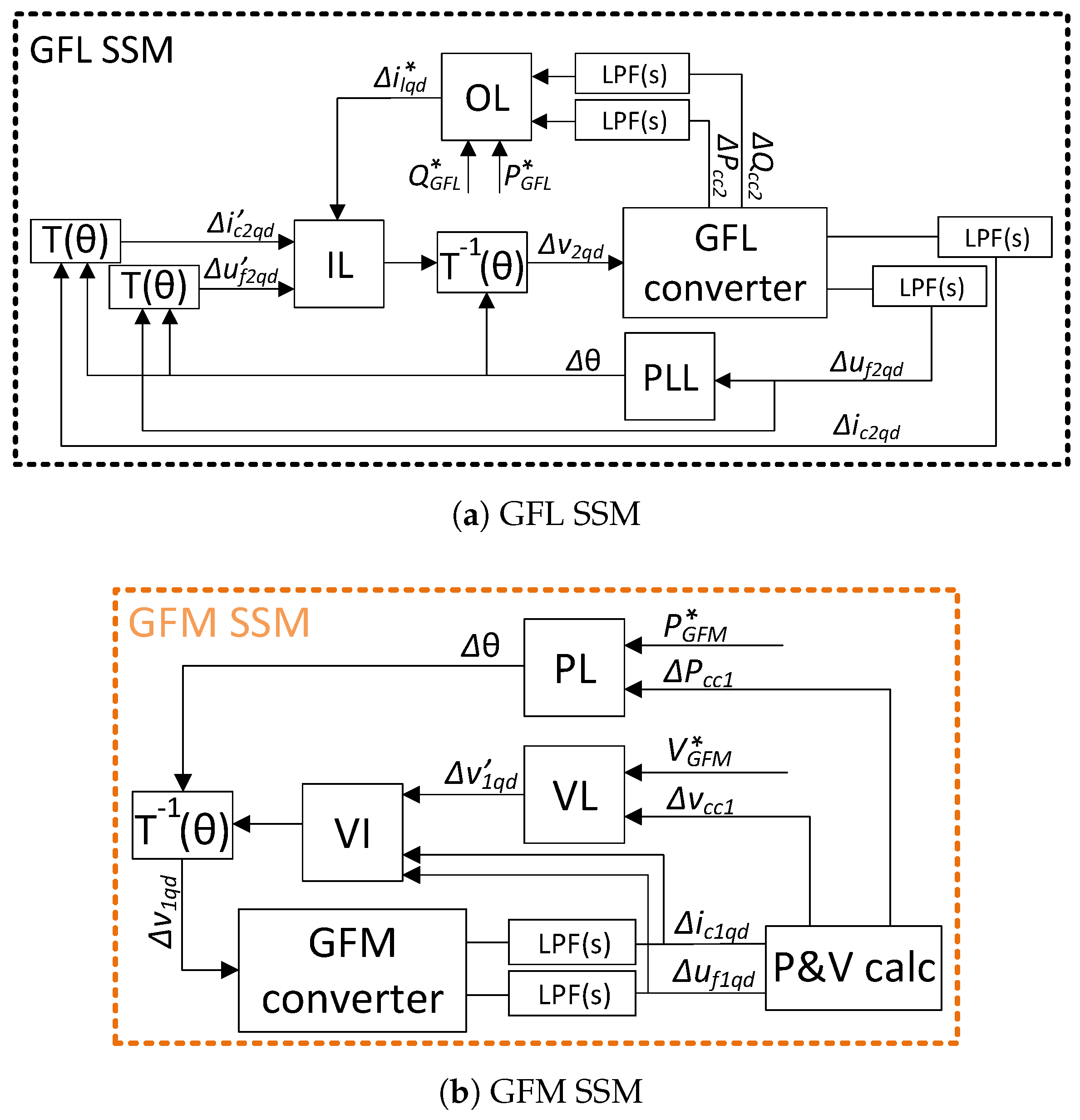
The controllers depicted in Figure 5 were linearized. The linearization process of these units is shown in Figure 6. Each component of both controllers (GFL in Figure 6a and GFM in Figure 6b) was first linearized independently, and then interconnected based on their respective inputs and outputs.

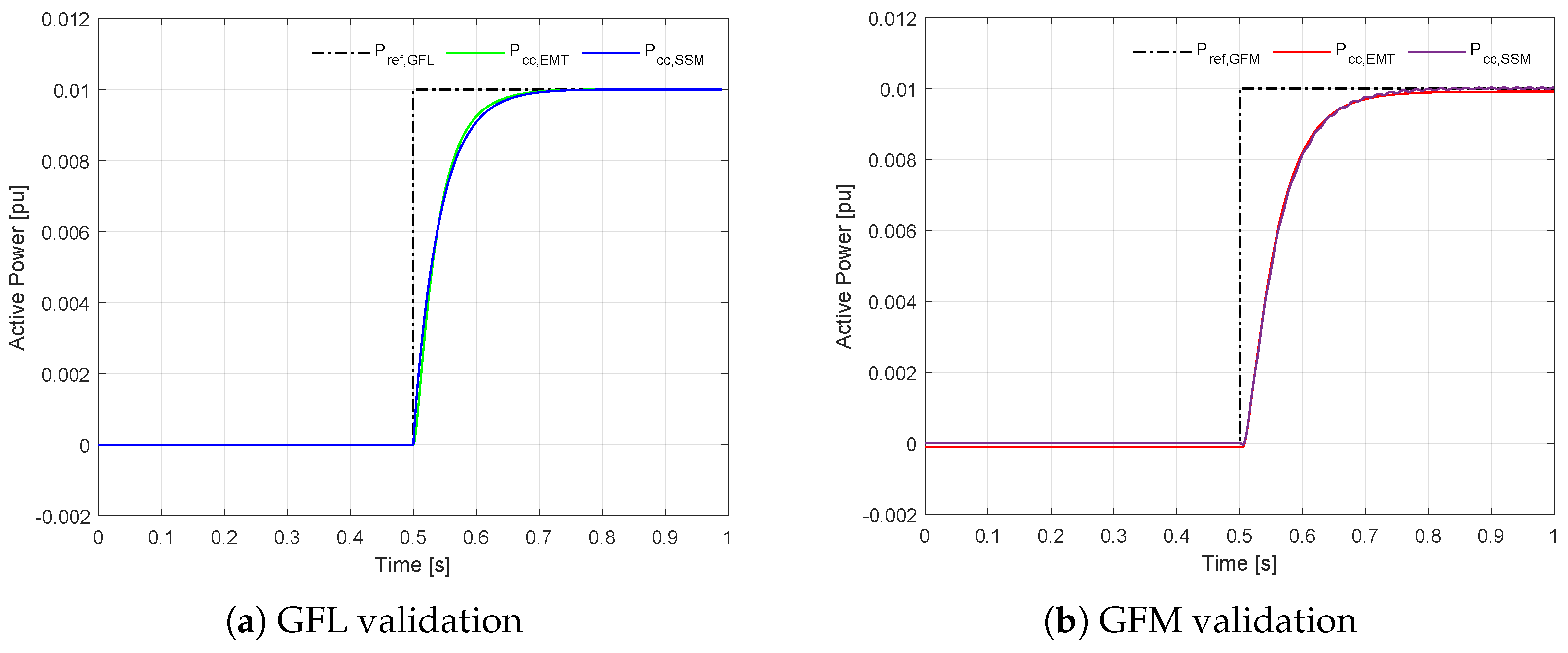
4.2. Small-Signal Model Validation

After developing the small-signal model (SSM), the initial step involved validating its accuracy by comparing it with the developed EMT model. For this validation, a single power step of 0.01 pu was applied to both EMT and SSM simulations. Figure 7 displays the results for both the GFL (Figure 7a) and GFM (Figure 7b) converter controllers for a cable length of 80 km and configuration A2. The same process was followed for the other two arrangements. The close alignment between the SSM and EMT responses in these figures confirms that the SSM accurately replicates the EMT behavior, demonstrating its reliability for further analysis.

4.3. Stability Assessment

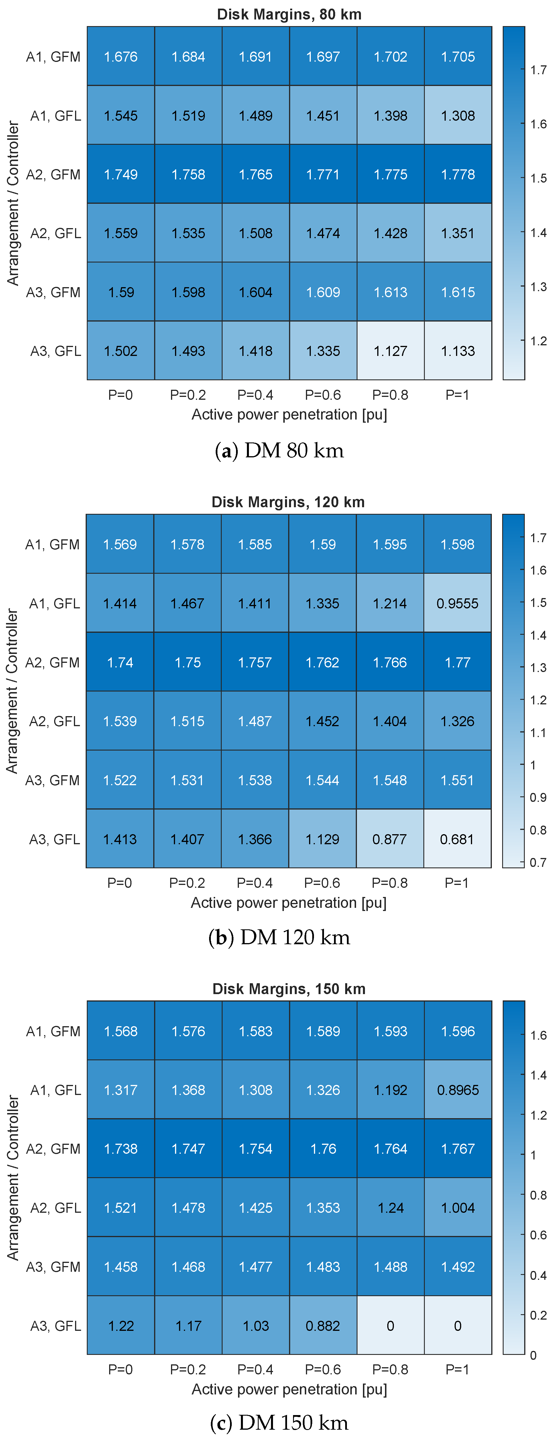
The disk margin analysis was conducted to assess the stability of the two converter control strategies, grid following and grid forming, across three distinct cable lengths: 80 km, 120 km, and 150 km, considering the three specific configurations labeled A1, A2, and A3. The results of the disk margins are shown in Figure 8 for 80 km (Figure 8a), 120 km (Figure 8b), and 150 km (Figure 8c).

Among these configurations, the grid-forming converter controller exhibited the largest disk margins, particularly in the A2 arrangement, followed by the A1 arrangement. This suggests that the GFM control strategy is more robust in maintaining stability than the GFL approach. This also suggests that distributing the shunt reactors along the export cable (A1 and A2), rather than having only one shunt compensation onshore (A3) further enhances stability.

The disk margins for the grid-forming controller remained consistent across all operating points, indicating reliable performance independent of active power variations. In contrast, the disk margins for the GFL controller demonstrated significant variability as the active power level increased from 0 to 1, with the lowest margins observed at higher active power penetration. Additionally, it was observed that an increase in cable length resulted in a decrease in disk margins, highlighting the influence of transmission distance, and hence, increased line impedance, on system stability. This reduction in disk margins corresponds to the Nyquist plot of the open-loop system moving closer to the critical −1 point as cable length and impedance increase, ultimately leading to conditions of marginal stability when the disk margin reaches zero. At this point, the system is unable to tolerate any uncertainty, and any additional perturbation could cause instability.

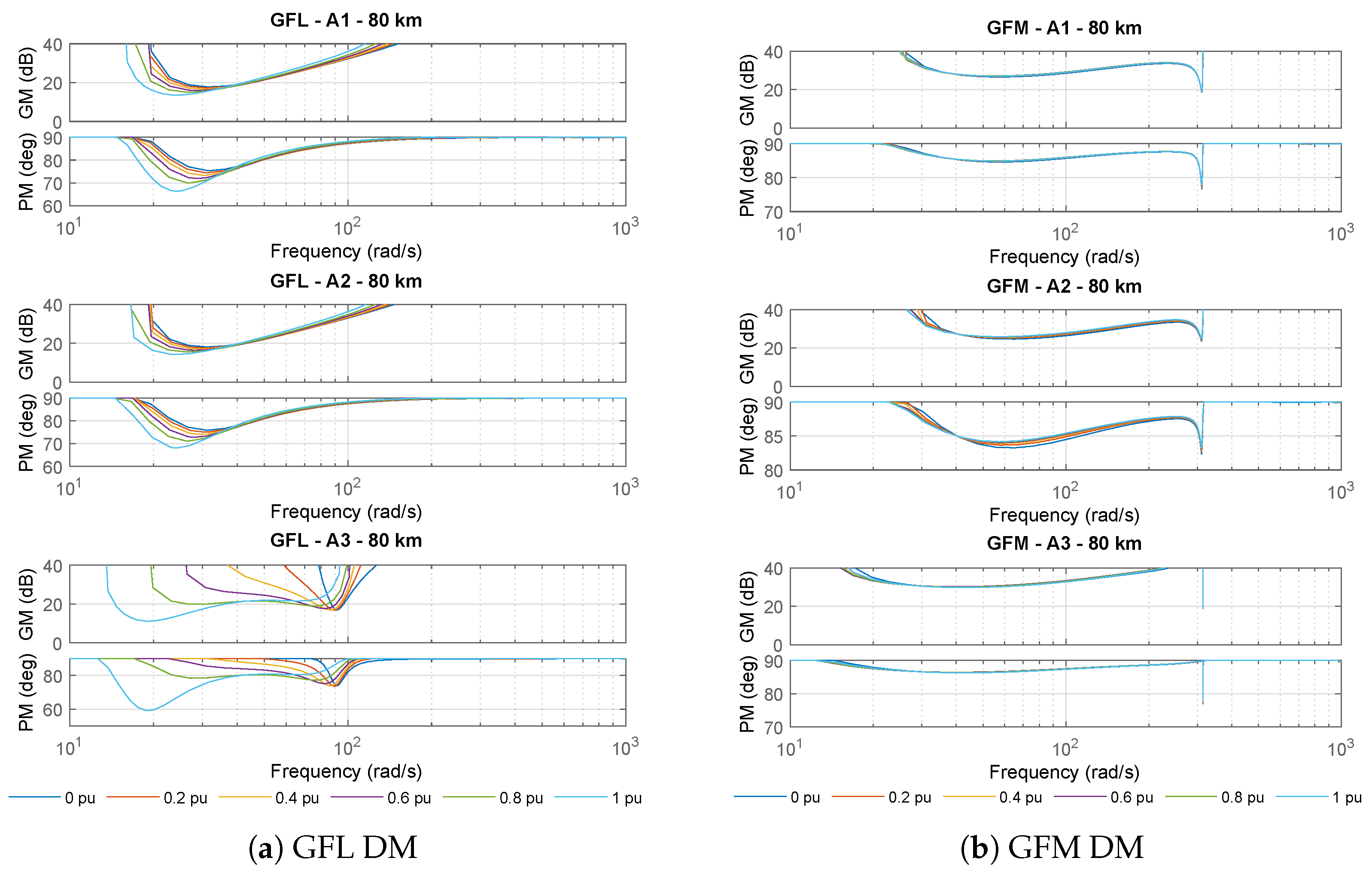
Figure 9 shows the gain and phase margins across a frequency spectrum where these margins are observed to be at their lowest. This analysis includes both GFL (Figure 9a) and GFM (Figure 9b) scenarios. The plots highlight the variation in the disk margins for the three different arrangements, specifically for a cable length of 80 km. Although only the 80 km case is depicted, similar trends are observed for cable lengths of 120 km and 150 km.

The plots reveal that, in the GFL scenario, the active power operating points significantly influence both the gain and phase margins. For configurations A1 and A2 within the GFL scenario, the lowest gain and phase margins, and consequently, the lowest disk margins are found at very low frequencies, specifically around 20 to 30 rad/s. These low-frequency disk margins are characterized by interactions between the GFL converter controller and the power system, especially due to the use of a PLL for grid synchronization and the inner current controller. In contrast, for configuration A3, there was a notable dip in both the gain and phase margins at frequencies below 20 rad/s, with an additional significant low point of approximately 90 rad/s.

In the GFM controller scenario, the gain and phase margins remained consistent across different operating points, corroborating previous observations. This consistency results in similar margin values across the entire frequency range. However, the lowest gain and phase margins for all three configurations occur at the natural frequency of the power system, likely due to interactions between the controller and the electrical grid. The 50 Hz peak can be further reduced by adjusting the values of the virtual impedance, specifically $R_v$ and $L_v$. However, this approach may result in reduced margins at lower frequencies. Therefore, future work should focus on optimizing the tuning of the virtual impedance to achieve greater mitigation of the gain and phase dips while preserving acceptable margins across the frequency spectrum.

The plots also highlight the influence of system arrangements on the gain and phase margins. The manner in which the controller interacts with the power system varies depending on the configuration, which plays a critical role in determining the overall stability of the system.

From this section, it can be concluded that the GFM controller demonstrates superior stability. It remains stable and robust across all cable lengths and configurations. In addition, the stability of the overall system is not critically affected by active power injection, which is important given that the power injected by the OWPP varies considerably with wind conditions and resource availability.

By contrast, the stability of the GFL-connected converter is influenced by the injected active power, with lower stability margins observed at higher power levels. Its stability is also affected by the transmission line impedance, leading to reduced stability and significantly lower margins with increased cable length.

Regarding the system configurations, arrangement A2 proved to be the most effective, followed by A1. This suggests that distributed shunt reactors across the transmission system enhance the stability, allowing for the use of longer cables.

It is important to note that this study was conducted using a weak grid with an SCR of 3. Further research should explore stronger networks, as the system might benefit from GFL controllers in scenarios with a stronger grid, where a robust voltage reference signal could enhance the GFL controller performance. However, since this study focuses on weaker grids, the next section will examine even weaker grids by varying the SCR and X/R ratio.

5. GFM and GFL Controllers Comparison for an HVAC-Connected OWPP in Weaker Networks

The integration of RESs into electrical power systems leads to significant changes in the grid dynamics. One of the challenges associated with this transition is the reduction in system strength, which is often quantified using SCR and X/R. These quantities reflect the ability of the grid to absorb disturbances and power delivery performance.

Section 4 focuses on the stability of the two controllers, different arrangements and the three cable lengths in a grid with an SCR of 3 and an X/R of 10 ($X_g/R_g$). Although this SCR value is already indicative of a relatively weak grid [39,40], further analysis is necessary to understand the performance and robustness of these controllers under even more challenging conditions. HVAC transmission introduces additional impedance as well as shunt reactors, and it was observed from the previous section that the different arrangements would benefit from different margins of stability. This effect becomes more noticeable in systems with lower SCR and X/R values. 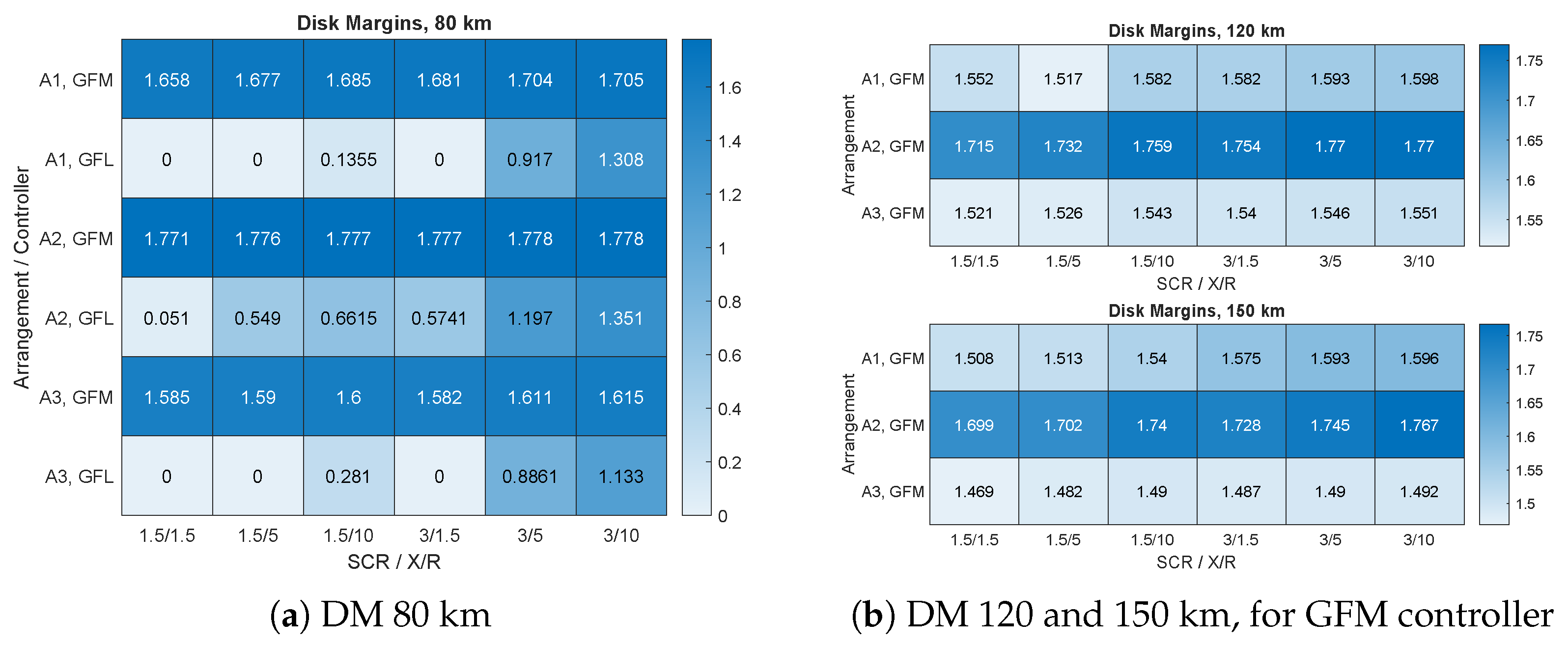An analysis similar to that in Section 4 was conducted. However, instead of varying the active power injection, the SCR (1.5 and 3), defined between the transmission system and the electrical grid, and X/R ratio (1.5, 5, and 10) were varied at the active power operating point of 1 pu. This specific operating point was chosen because it previously showed lower stability margins in the GFL case, making it a critical point of interest.

Figure 10a shows the disk margins for different configurations, A1, A2, and A3, under both controllers, with an HVAC transmission length of 80 km. The results confirm the findings from Section 4—GFM control, which improves the stability and robustness in weaker grids. The lower X/R and SCR values did not significantly affect the disk margins of this controller. This can also be observed in Figure 11b, which shows that the disk margins maintain a consistent gain and phase across all X/R and SCR values. The pole-zero map in this figure further illustrates these effects, where it can be seen that the system remains stable, with no poles on the right-half plane. The pole-zero map was used here, as it was necessary to display the instabilities of the GFL scenario, where even for an 80 km transmission with arrangement A2, which performs best, the system becomes unstable. As seen in Figure 11a, the system is already unstable at X/R = 1.5 and SCR = 1.5, and nearly unstable at SCR = 3 and X/R = 1.5, with a pole close to the origin. The pole-zero maps clearly demonstrate how X/R and SCR impact stability, with poles shifting to the right as SCR and X/R decrease. The findings in Figure 10b show that nearly all disk margins are unstable for the GFL controller under these conditions, particularly for 80 km of transmission. Therefore, GFM converter units are essential for longer HVAC transmissions, especially in weaker grids with higher impedances.

The GFM-connected controller showed consistent performance across different X/R and SCR values, even with longer cables of 120 and 150 km, as shown in Figure 10b. The results also indicate that arrangement A2 is the most effective, supporting the conclusion from the previous section that distributing shunt reactors along the line significantly improves the stability.

In conclusion, GFM is necessary for longer export cables, particularly in weaker grids with lower X/R and SCR values. Configuration A2 is recommended for enhanced stability, although configuration A1 has also been proven to be robust across all GFM operating points.

6. Discussion

The results presented in Section 4 and Section 5 illustrate the comparative performance of GFL and GFM controllers for OWPPs connected via HVAC export cables.

Table 3. Advantages and disadvantages of GFL and GFM control strategies based on the paper findings.

Criteria	Grid-Following (GFL)	Grid-Forming (GFM)
Advantages	- Simple and widely adopted in current OWPP systems. - Effective in strong grids with higher short-circuit ratios. - Easier to implement with conventional systems.	- Superior stability and robustness across all cable lengths. - Performs well in weak grids (low SCR and X/R ratios). - Stability is independent of active power injection levels. - Supports operation in island mode and black-start scenarios.
Disadvantages	- Stability is highly sensitive to active power injection. - Poor performance with weak grids and longer HVAC cables. - Low disk margins at high power levels and weaker SCR values. - Requires strong voltage reference for synchronization.	- Requires more complex control and tuning processes. - Not yet widely deployed in OWPP systems. - Slightly higher computational demands due to VSM approach. - Needs further research for industrial adoption.

summarizes the advantages and disadvantages of both strategies, providing an overview of their characteristics based on the findings.

GFM controllers demonstrate superior stability and robustness across all system configurations and cable lengths. This is evident in Figure 8, which shows that the GFM control strategy consistently achieves higher $\alpha$ values for all three cable lengths, maintaining stability across all active power operating points analyzed. In contrast, the GFL controller exhibits a significant loss of stability as cable lengths increase. For the 150 km cable, some operating points already display a disk margin of zero, indicating no tolerance for uncertainty. In such cases, the factor f equals 1, meaning even a small uncertainty or disturbance would result in instability.

The disk margin analysis also highlights the consistent performance of GFM under weak grid conditions with low SCR and varying X/R ratios. This robustness can be attributed to the independence of GFM control from grid synchronization, allowing it to maintain stability even under significant active power variations. Conversely, GFL controllers show pronounced stability limitations, particularly as active power injection increases. These limitations are exacerbated by weaker grid conditions and increased cable lengths. Figure 10 further emphasizes the superiority of GFM, particularly for weaker systems. Even with a shorter 80 km cable, the GFL controller demonstrates zero $\alpha$ values across all configurations and active power penetration levels, underscoring its inability to maintain stability in such conditions.

While GFL remains simpler to implement and is widely adopted in current systems, its performance is heavily reliant on grid strength and a robust voltage reference. These limitations are reflected in the reduced disk margins observed at higher power levels and weaker grid conditions. In contrast, GFM provides a reliable solution for OWPP applications requiring extended HVAC export cables, effectively mitigating stability challenges associated with line impedance and reactive power imbalance.

Despite its superior performance, the adoption of GFM controllers remains limited due to the need for further research and development. Future work should focus on addressing these challenges to accelerate the integration of GFM controllers in offshore wind applications, thereby enhancing grid stability and enabling reliable operation under increasingly demanding conditions.

7. Conclusions

As fossil fuels are phased out in favor of renewable energy sources, the dynamics of power systems are undergoing significant change. The OWPP, a key component of this shift, are being commissioned at increasing distances from shore. Owing to the maturity and reliability of HVAC cables, they are the preferred choice for these connections. However, as these cables extend further offshore, reactive power compensation is necessary to ensure the system stability.

Currently, most connected offshore wind farms operate in grid-following mode. This study compares the performance of three cable lengths—80 km, 120 km, and 150 km—for an OWPP connected to a local network, with an HVAC cable utilizing shunt reactors to compensate for capacitive reactive power. Three specific configurations were analyzed: A1, with shunt reactors located at both the offshore substation and onshore; A2, similar to A1 but with an additional mid-cable reactor; and A3, with a shunt reactor only onshore.

The study also compared cable lengths and configurations under two different control strategies: GFL and GFM. The primary goal was to identify the optimal system arrangement and control strategy to enhance the stability and robustness, as assessed through a small-signal model.

The findings indicate that across all cable lengths, the most robust configuration is configurations A2 when paired with GFM control, followed by arrangement A1 with the same control strategy. The GFM control significantly enhanced the system stability compared to the GFL converter controller. It maintained consistent stability across a range of power operating points, from 0 to 1 pu penetration, for all cable lengths. In contrast, the stability of the GFL unit is highly dependent on the level of active power injected into the grid.

In addition, an analysis was conducted for weaker grids with lower SCR and X/R values. The results confirmed that GFM-connected controllers are the preferred option, as they maintain consistent disk margins across all SCR and X/R values. In contrast, the GFL controller was unable to maintain stability in weaker networks, even at a shorter transmission distance of 80 km.

The results suggest that GFM control holds potential for OWPPs located further from the shore. The inclusion of reactors at offshore substation, and mid-cable for enhanced stability, is recommended. Additionally, the GFM unit demonstrated independence from grid stiffness, performing well in weaker grids with lower SCR and lower X/R. On the other hand, GFL units struggled to maintain stability under these conditions, often becoming unstable, as indicated by a disk margin of zero. These findings reinforce the recommendation to employ GFM control in OWPP applications.

References

1. Díaz, H.; Guedes Soares, C. Review of the current status, technology and future trends of offshore wind farms. Ocean Eng. 2020, 209, 107381. [Google Scholar] [CrossRef]
2. Komusanac, I.; Brindley, G.; Fraile, D.; Ramirez, L. Wind Energy in Europe: 2021 Statistics and the Outlook for 2022–2026; WindEurope: Brussels, Belgium, February 2022. [Google Scholar]
3. Elliott, D.; Bell, K.R.; Finney, S.J.; Adapa, R.; Brozio, C.; Yu, J.; Hussain, K. A Comparison of AC and HVDC Options for the Connection of Offshore Wind Generation in Great Britain. IEEE Trans. Power Deliv. 2016, 31, 798–809. [Google Scholar] [CrossRef]
4. Rahman, S.; Khan, I.; Alkhammash, H.I.; Nadeem, M.F. A comparison review transmission mode for onshore integration of offshore wind farms: HVDC or HVAC. Electronics 2021, 10, 1489. [Google Scholar] [CrossRef]
5. Xie, S.; Wang, X.; Qu, C.; Wang, X.; Guo, J. Impacts of different wind speed simulation methods on conditional reliability indices. Int. Trans. Electr. Energy Syst. 2013, 20, 359–373. [Google Scholar] [CrossRef]
6. Kalair, A.; Abas, N.; Khan, N. Comparative study of HVAC and HVDC transmission systems. Renew. Sustain. Energy Rev. 2016, 59, 1653–1675. [Google Scholar] [CrossRef]
7. Khalilnezhad, H.; Chen, S.; Popov, M.; Bos, J.A.; De Jong, J.P.; Van Der Sluis, L. Shunt compensation design of EHV doublecircuit mixed OHL-cable connections. In Proceedings of the IET International Conference on Resilience of Transmission and Distribution Networks (RTDN) 2015, Birmingham, UK, 22–24 September 2015. [Google Scholar] [CrossRef]
8. Song-Manguelle, J.; Todorovic, M.H.; Chi, S.; Gunturi, S.K.; Datta, R. Power transfer capability of HVAC cables for subsea transmission and distribution systems. IEEE Trans. Ind. Appl. 2014, 50, 2382–2391. [Google Scholar] [CrossRef]
9. Jansen, K.; Van Hulst, B.; Engelbrecht, C.; Hesen, P.; Velitsikakis, K.; Lakenbrink, C. Resonances due to long HVAC offshore cable connections: Studies to verify the immunity of Dutch transmission network. In Proceedings of the 2015 IEEE Eindhoven PowerTech (PowerTech 2015), Eindhoven, The Netherlands, 29 June–2 July 2015; pp. 1–6. [Google Scholar] [CrossRef]
10. Mytilinou, V.; Kolios, A.J. Techno-economic optimisation of offshore wind farms based on life cycle cost analysis on the UK. Renew. Energy 2019, 132, 439–454. [Google Scholar] [CrossRef]
11. Gustavsen, B.; Mo, O. Variable transmission voltage for loss minimization in long offshore wind farm AC export cables. IEEE Trans. Power Deliv. 2017, 32, 1422–1431. [Google Scholar] [CrossRef]
12. Dui, X.W.; Zhu, G.P. Reactive compensation research of HVAC cables for offshore wind farms. Adv. Mater. Res. 2014, 986–987, 433–438. [Google Scholar] [CrossRef]
13. Rashid, M.H. Power Electronics Handbook, 3rd ed.; Elsevier Inc.: New York, NY, USA, 2011. [Google Scholar] [CrossRef]
14. Di Bartolomeo, E.; Di Giulio, A.; Palone, F.; Rebolini, M.; Iuliani, V. Terminal stations design for submarine HVAC links Capri-Italy and Malta-Sicily interconnections. In Proceedings of the 2015 AEIT International Annual Conference (AEIT 2015), Naples, Italy, 14–16 October 2015. [Google Scholar] [CrossRef]
15. Lauria, S.; Palone, F. Optimal operation of long inhomogeneous AC cable lines: The malta-sicily interconnector. IEEE Trans. Power Deliv. 2014, 29, 1036–1044. [Google Scholar] [CrossRef]
16. Lauria, S.; Schembari, M.; Palone, F.; Maccioni, M. Very long distance connection of gigawattsize offshore wind farms: Extra high-voltage AC versus high-voltage DC cost comparison. IET Renew. Power Gener. 2016, 10, 713–720. [Google Scholar] [CrossRef]
17. Wiechowski, W.; Eriksen, P.B. Selected studies on offshore wind farm cable connections—Challenges and experience of the Danish TSO. In Proceedings of the IEEE Power and Energy Society 2008 General Meeting: Conversion and Delivery of Electrical Energy in the 21st Century (PES), Pittsburgh, PA, USA, 20–24 July 2008. [Google Scholar] [CrossRef]
18. Dakic, J.; Cheah, M.; Prieto-Araujo, E.; Gomis-Bellmunt, O. Optimal sizing and location of reactive power compensation in offshore HVAC transmission systems for loss minimization. In Proceedings of the 18th Wind Integration Workshop, Dublin, Ireland, 16–18 October 2019; pp. 1–6. [Google Scholar]
19. Dakic, J.; Cheah-Mane, M.; Gomis-Bellmunt, O.; Prieto-Araujo, E. HVAC Transmission System for Offshore Wind Power Plants including Mid-Cable Reactive Power Compensation: Optimal Design and Comparison to VSC-HVDC Transmission. IEEE Trans. Power Deliv. 2021, 36, 2814–2824. [Google Scholar] [CrossRef]
20. Zuo, Y.; Yuan, Z.; Sossan, F.; Zecchino, A.; Cherkaoui, R.; Paolone, M. Performance assessment of grid-forming and grid-following converter-interfaced battery energy storage systems on frequency regulation in low-inertia power grids. Sustain. Energy Grids Netw. 2021, 27, 100496. [Google Scholar] [CrossRef]
21. Pattabiraman, D.; Lasseter, R.H.; Jahns, T.M. Comparison of Grid Following and Grid Forming Control for a High Inverter Penetration Power System. In Proceedings of the 2018 IEEE Power & Energy Society General Meeting (PESGM), Portland, OR, USA, 5–10 August 2018; pp. 3–7. [Google Scholar] [CrossRef]
22. Jain, A.; Sakamuri, J.; Cutululis, N. Grid-forming control strategies for blackstart by offshore wind farms. Wind. Energy Sci. 2020, 5, 1297–1313. [Google Scholar] [CrossRef]
23. Wang, Z.; Hibberts-Caswell, R.; Oprea, L. Comparison of Grid-Following and Grid-Forming Control in Weak AC System. In Proceedings of the 2021 International Conference on Electrical, Computer and Energy Technologies (ICECET), Cape Town, South Africa, 9–10 December 2021; pp. 1–5. [Google Scholar] [CrossRef]
24. Du, W.; Tuffner, F.K.; Schneider, K.P.; Lasseter, R.H.; Xie, J.; Chen, Z.; Bhattarai, B. Modeling of Grid-Forming and Grid-Following Inverters for Dynamic Simulation of Large-Scale Distribution Systems. IEEE Trans. Power Deliv. 2021, 36, 2035–2045. [Google Scholar] [CrossRef]
25. Unruh, P.; Nuschke, M.; Strauß, P.; Welck, F. Overview on grid-forming inverter control methods. Energies 2020, 13, 2589. [Google Scholar] [CrossRef]
26. Rosso, R.; Engelken, S.; Liserre, M. Robust Stability Investigation of the Interactions among Grid-Forming and Grid-Following Converters. IEEE J. Emerg. Sel. Top. Power Electron. 2020, 8, 991–1003. [Google Scholar] [CrossRef]
27. Morris, J.F.; Ahmed, K.H.; Egea, A. Standardized Assessment Framework for Design and Operation of Weak AC Grid-Connected VSC Controllers. IEEE Access 2021, 9, 95282–95293. [Google Scholar] [CrossRef]
28. Henderson, C.; Egea-Alvarez, A.; Xu, L. Analysis of multi-converter network impedance using MIMO stability criterion for multi-loop systems. Electr. Power Syst. Res. 2022, 211, 108542. [Google Scholar] [CrossRef]
29. Shah, S.; Gevorgian, V. Control, Operation, and Stability Characteristics of Grid-Forming Type III Wind Turbines Preprint. In Proceedings of the 19th Wind Integration Workshop, Ljubljana, Slovenia, 11–13 November 2020. [Google Scholar]
30. Du, W.; Chen, Z.; Schneider, K.P.; Lasseter, R.H.; Pushpak Nandanoori, S.; Tuffner, F.K.; Kundu, S. A Comparative Study of Two Widely Used Grid-Forming Droop Controls on Microgrid Small-Signal Stability. IEEE J. Emerg. Sel. Top. Power Electron. 2020, 8, 963–975. [Google Scholar] [CrossRef]
31. Paquette, A.D.; Divan, D.M. Virtual Impedance Current Limiting for Inverters in Microgrids With Synchronous Generators. IEEE Trans. Ind. Appl. 2015, 51, 1630–1638. [Google Scholar] [CrossRef]
32. Lu, X.; Wang, J.; Guerrero, J.M.; Zhao, D. Virtual-impedance-based fault current limiters for inverter dominated AC microgrids. IEEE Trans. Smart Grid 2018, 9, 1599–1612. [Google Scholar] [CrossRef]
33. Wang, X.; Li, Y.W.; Blaabjerg, F.; Loh, P.C. Virtual-Impedance-Based Control for Voltage-Source and Current-Source Converters. IEEE Trans. Power Electron. 2015, 30, 7019–7037. [Google Scholar] [CrossRef]
34. Rodriguez-Cabero, A.; Roldan-Perez, J.; Prodanovic, M. Virtual Impedance Design Considerations for Virtual Synchronous Machines in Weak Grids. IEEE J. Emerg. Sel. Top. Power Electron. 2020, 8, 1477–1489. [Google Scholar] [CrossRef]
35. Henderson, C.; Egea-Alvarez, A.; Fekriasl, S.; Knueppel, T.; Amico, G.; Xu, L. The Effect of Grid-Connected Converter Control Topology on the Diagonal Dominance of Converter Output Impedance. IEEE Open Access J. Power Energy 2023, 10, 617–628. [Google Scholar] [CrossRef]
36. Henderson, C.; Egea-Alvarez, A.; Xu, L. Analysis of optimal grid-forming converter penetration in AC connected offshore wind farms. Int. J. Electr. Power Energy Syst. 2024, 157, 109851. [Google Scholar] [CrossRef]
37. Seiler, P.; Packard, A.; Gahinet, P. An Introduction to Disk Margins [Lecture Notes]. IEEE Control Syst. 2020, 40, 78–95. [Google Scholar] [CrossRef]
38. Egea-Alvarez, A.; Fekriasl, S.; Hassan, F.; Gomis-Bellmunt, O. Advanced Vector Control for Voltage Source Converters Connected to Weak Grids. IEEE Trans. Power Syst. 2015, 30, 3072–3081. [Google Scholar] [CrossRef]
39. Ahmed, M.; Meegahapola, L.; Vahidnia, A.; Datta, M. Analyzing the Effect of X/R ratio on Dynamic Performance of Microgrids. In Proceedings of the 2019 IEEE PES Innovative Smart Grid Technologies Europe (ISGT-Europe 2019), Bucharest, Romania, 29 September–2 October 2019; pp. 1–5. [Google Scholar] [CrossRef]
40. Alizadeh, S.M.; Ozansoy, C.; Alpcan, T. The impact of X/R ratio on voltage stability in a distribution network penetrated by wind farms. In Proceedings of the 2016 Australasian Universities Power Engineering Conference (AUPEC), Brisbane, QLD, Australia, 25–28 September 2016; pp. 1–6. [Google Scholar] [CrossRef]
Figure 1. One-line diagram of an OWPP connected via an HVAC transmission system to the electrical grid.
Electricity 06 00004 g001
Figure 2. Model of the aggregated offshore wind farm and its connection to the electrical grid.
Electricity 06 00004 g002
Figure 3. Voltage profile for an 80 km HVAC export cable for A0 (no compensation), A1, A2, and A3.
Electricity 06 00004 g003
Figure 4. Impact of varying SCR and X/R in the voltage profile for an 80 km HVAC export cable.
Electricity 06 00004 g004
Figure 5. Schematic of both GFL (a) and GFM (b) converter controllers.
Electricity 06 00004 g005
Figure 6. Scheme of linearized system (SSM) for GFM and GFL converter controllers.
Electricity 06 00004 g006
Figure 7. Validation of SSM against EMT results for a 0.01 pu active power jump.
Electricity 06 00004 g007
Figure 8. Disk margins for active power operating points and for both GFM/GFL controllers and different system arrangements.
Electricity 06 00004 g008
Figure 9. Gain and phase disk margins across the frequency spectrum.
Electricity 06 00004 g009
Figure 10. Disk margins for different SCR and X/R.
Electricity 06 00004 g010
Figure 11. Gain and phase disk margins across the frequency spectrum for SCR and X/R variation.
Electricity 06 00004 g011