Power System Impacts of Electric Vehicle Charging Strategies

Abstract

This article explores the potential impacts of integrating electric vehicles (EVs) and variable renewable energy (VRE) on power system operation. EVs and VRE are integrated in a production cost model with a 5 min time resolution and multiple planning horizons to deduce the effects of variable generation and EV charging on system operating costs, EV charging costs, dispatch stacks, reserves and VRE curtailment. EV penetration scenarios of the light-duty vehicle fleet of 10%, 20%, and 30% are considered in the RTS-GMLC test system, and VRE penetration is 34% of annual energy consumption. The impacts of EVs are investigated during the annual peak in the summer and during the four weeks of the year in which high VRE and low loads lead to overgeneration. Uncoordinated and coordinated EV charging scenarios are considered. In the uncoordinated scenario, charging is undertaken at the convenience of the EV owners, modeled using data from the Idaho National Laboratory’s EV Project. Coordinated charging uses an “aggregator” model, wherein EV charging is scheduled to minimize operating costs while meeting the daily charging requirements subject to EV availability and charging constraints. The results show that at each EV penetration level, the uncoordinated charging costs were higher than the coordinated charging costs. During a high-VRE, low-load week, with uncoordinated EV charging at 30% penetration (3% energy penetration), the peak load increased by as much as 27%. Using coordinated charging, the EV load shifts to hours with low prices, coincident with either low load, high VRE, or both. Furthermore, coordinated charging substantially reduces the curtailment of PV by as much as nine times during the low-load seasons, and the curtailment of wind generation by more than half during the summer peak season, compared to the scenarios with no EVs and uncoordinated EV charging. Using a production cost model with multiple planning cycles, load and VRE forecasts, and a “look ahead” period during scheduling and dispatching units was crucial in creating and utilizing the flexibility of coordinated EV charging.

1. Introduction

Climate change has driven many governments and organizations to set ambitious clean energy goals, seeking to achieve significant reductions in carbon emissions by 2035 and to achieve carbon neutrality by mid-century, e.g., Hawaii’s 100% clean energy standard, California’s standard [1], the European Union [2], and organizations such as Google [3], Walmart [4], Amazon [5], etc. In the electrical supply system, decarbonization will be centered upon renewable energy resources, primarily wind and solar due to their low costs [6], but also nuclear power, energy storage [7], dynamic and controllable loads, and market innovations [8]. In 2020, the U.S. Energy Information Agency (EIA) reported that 36% percent of CO₂ emissions were due to the transportation sector [9]. Consequently, for decarbonization to occur, the transportation sector must decarbonize.

Potential paths to decarbonize transportation include carbon-neutral biofuels, hydrogen fuel cells, and electric vehicles (EVs), among others. For vehicle transportation, EVs are the most likely path to decarbonization. According to the U.S. National Renewable Energy Laboratory (NREL), the levelized cost of driving (LCOD), with no tax credits or incentives, for some conventional vehicles and EVs has been the same since 2021 [10]. For example, the estimated cost of driving after eight years is the same for a Tesla Model 3 Standard Range and a Toyota Camry XLE [11]. One of the most important drivers in the cost of a modern EV is the battery pack, which may account for up to 40% of the cost [12]. In 2020, on a per unit energy basis, battery packs cost USD 137/kWh, representing a reduction of 89% from 2010 to 2020 [13], and further decreases are expected. Thus, it is likely that EVs will represent a larger share of the car fleet soon. Sales continues to rise and in 2021, the EV sales worldwide doubled from the 2020 numbers, achieving more than a 6% market share [14], while in the U.S. sales also doubled from the 2020 numbers, with a market share of 4% [15]. Some have projected that 75% of the sales of light-duty vehicles will be electric by 2050 [16].

1.1. Penetration Levels of EVs

In 2020, EV penetration into the light-duty vehicle fleet in the U.S. was 2%, equivalent to 1.7 million EVs [17]. EV sales are experiencing continuous growth, and from 2011 to 2017 the average sales rate grew by 49% [18]. In 2018, the sales growth rate was 80% [19]. During 2021 in the U.S., EV sales doubled from the 2020 numbers, achieving an LDV market share of 4% [15]. Higher levels of penetration are expected in future years. For example, in California, zero-emission vehicle (ZEV) regulations require a minimum number of EV sales, which should reach 22% of DV sales by 2025 [20]. This mandate is established by a California Executive Order and requires up to 1.5 million ZEVs by 2025 [21]. A study by the National Renewable Energy Laboratory (NREL) suggested that under a scenario of high policy support for consumer adoption, up to 84% of the light-duty vehicle (LDV) fleet can be occupied EVs by 2050, and 20% of LDVs by 2030 [22]. Furthermore, the International Renewable Energy Association (IRENA) estimates that 30% of the worldwide vehicle fleet will be made electric by 2030 [23]. The International Energy Agency (IEA) suggested in its Global Energy Outlook that 10% of the vehicle fleet could be made electric by 2030 [24].

Table 1. Expected EV penetration by 2030 in the U.S. and globally.

Source	Location	Penetration	Year
IEA	Global	10%	2030
NREL	U.S.	20%	2030
IRENA	Global	30%	2030

summarizes these potential EV penetration levels by 2030. Based upon these forecasts, this work investigates the impacts of light-duty EV penetration scenarios of 10%, 20% and 30%.

1.2. EV Literature Review

Automakers have committed to transitioning their fleets from internal combustion vehicles to EVs over the coming decades [25]. Given that the electricity sector is on a path toward decarbonization, EVs will eventually derive their energy from carbon-free resources. Because of their ability to use carbon-free energy and due to their good performance and low operating costs, the wide-scale adoption of EVs is expected as they achieve first-cost price parity with conventional internal combustion vehicles, which is expected to occur later this decade [26].

In “The Rise of the Electric Vehicles—2020 Status and Future Expectations” [27], Muratori presents an extended literature review and classifies the articles according to the following seven topics:

• Light-duty EV market and adoption projections;
• Insights on market opportunities beyond light-duty EVs;
• Performance evolution for key EV components such as batteries;
• Charging infrastructure status and modeling;
• EV charging impacts ranging from bulk power system operation to distribution networks;
• EV life-cycle cost and emissions studies;
• Future expectations and synergies between EV and other technologies.

These classifications provide a convenient breakdown for organizing previous works. This paper deals primarily with topic (5), namely the impacts on the bulk power system, and consequently the literature review will be focused in this area.

The transition from internal combustion engines to electric vehicles in the transportation sector will lead to an increase in power demand in the electric sector [28]. In doing so, it is crucial to avoid increases in the peak load and to maintain affordable electricity [29]. For example, there is evidence that the uncoordinated charging of EVs can increase the peak load, or possibly introduce a second peak during off-peak hours [30]. However, if it is coordinated, EV charging can also enhance the penetration of variable renewable energy such as wind and solar power [31].

Mo et al. [32] presented updates related to the topics of light-duty EV markets (1), charging infrastructure status (4), emissions (6) and emerging technologies (7). They identified that the main challenge for EV users is the lack of charging infrastructure and its poor management. Therefore, their work is a guide for advocating EVs in dense metropolitan cities around the globe.

Regarding charging impacts in distribution networks, Jones et al. [33] used an alternating current power flow (ACPF) model to study the impacts on voltage and line loading and concluded that EVs will increase the peak load in the distribution system specially on residential feeders. Schulz et al. [34] used a 15 min time resolution “direct current unit commitment optimal power flow” model focused on the optimization of the energy consumption and cost of a household in a distribution network. They concluded that optimization at the household level improves system operation when distributed energy systems can access wholesale electricity prices.

Recent work on the topic of integrating EVs has analyzed the effects of EVs when their charging is included in the day ahead (DA) market by using a production cost model (PCM). Regarding bulk power system optimization, Szinai et al. performed monthly simulations of power system operations for a whole year [35]. EV modeling comes from a bottom-up analysis, in which a portion is flexible and the rest is inflexible. Their model represents the U.S. Western Interconnection zonally and focuses on California in 2025, assuming an EV fleet ranging from 0.95 to 5 million cars. Their model neglects intraday commitments, i.e., it models only the day-ahead (DA) market. In this simplified transmission system, EV flexible charging is modeled as an electric storage unit. The modeling assumes that storage is full at the beginning of each month (horizon), and the model load is shifted by not charging at peak hours and charging at times with low electricity prices. Their main conclusion is that charging of the EV fleet (flexible and inflexible) increases the total power system operation cost by up to 10% (USD 690 million), but it also reduces the VRE curtailment by up to 40% annually. The study also found that utilizing TOU rates instead of flexible charging led to a similar production cost but does not provide curtailment reductions.

Another work regarding the integration of EVs into the bulk power system is from Mowry and Mallapragada [36]. They focused on highway fast charging, which has a high power requirement, modeled as an inflexible load along intercity highways in the ERCOT power system in 2033. The central case evaluated an EV fleet of 3 million LDVs, with low and high scenarios of 1.5 to 4.5 million LDVs. They used a grid operation model (PCM) but with major simplifications, neglecting the procurement of reserves, and no intraday rescheduling of the thermal generation fleet in the power system. The DC fast charging station in the modeling assumed on-site electric battery storage units (lithium batteries). The demand flexibility in their work was up to 20 percent of the charging load and within a narrow window of 1 h. They concluded that 3 million EVs will increase the annual power system operation cost by 8%. In addition, based on their assumption that the EV load is inflexible and at the best case can be flexible only within an hour window, the use of a 4 h battery at the fast-charging stations is effective in reducing price spikes due to vehicle charging.

Alvarez Guerrero et al. [37] considered how to model EV charging for use in a PCM of power system operation. This work modeled the EV load assuming uncoordinated and coordinated charging models subject to the constraints of EV availability for charging, state-of-charge, and energy charging requirements. EV constraints were modeled based upon data from the Idaho National Laboratory’s EV Project [30]. EV charging constraints were incorporated directly into the PCM, thus accounting for EV charging flexibility, contrary to the work of [35], which used a storage device. Additionally, the model in [37] provides a single optimization inside the PCM for the sake of EV flexible charging without the iterative process between two optimization tools [36]. In addition, the work considered all types of charging levels, DC fast and residential, and employing no additional storage devices. Thus, in [37], cost savings associated with coordinated charging can be directly compared to the same fleet’s uncoordinated charging cost.

Muratori [38], in “The Shape of Electrified Transportation”, mentioned that studies related to the impacts of EV charging in the bulk power system do not provide flexibility for multiple days, i.e., only one day is analyzed. Additionally, studies do not guarantee the energy requirements for the EV fleet while also providing value to the power system, such as the reduction in the curtailment of renewable energies and the reduction in the power system’s peak demand.

1.3. Novelty and Contributions of the Current Work

The current work presented in this paper builds upon past work and includes important advances in the production cost modeling: first, the integration of EVs into the PCM modeled nodally (not zonally) and at a high time-resolution of 5 min. Additionally, the model includes multiple unit commitment planning horizons, from a week ahead to real-time, in which the impact of EV charging is determined while considering the multiday flexibility as described in [38]. Additionally, this article reports the use of the EV modeling approach from [37] but addresses the previous limitation of using perfect foresight and a single planning horizon, i.e., day ahead (DA), which was also the case in [35,36]. Thus, the modeling includes commitment decisions of a real power system in which some thermal units have a start time greater than a day, and where intraday rescheduling of combined-cycle and fast resources such as combustion turbines is possible. It is therefore possible to deal with forecast errors of VRE in the real-time (RT) market. In the RT market, all the commitments are final. The system operator dispatches generators based on actual weather conditions; only then can it calculate all of the expenses involved in running the power system. By including forecast errors, the model is able to capture the costs associated with handling such errors. The total costs in [35,36] are likely underestimated because their models do not compensate for the differences between the DA forecast and the actual RT conditions. Therefore, the modeling approach in this article simulates power system operation and total costs more realistically, and importantly allows the charging of EVs to be rescheduled or re-dispatched depending on updated forecasts and real-time conditions.

The purpose of the work herein is to present the setup and results of a power system production cost model that incorporates the full range of timing for unit commitment decisions (from week ahead to RT) in a power system that integrates a high penetration of electric vehicles (EVs) and variable renewable energies (VRE). Thus, this work targets the following specific research questions:

• What are the impacts of uncoordinated and coordinated EV charging strategies on power system operation, peak loads, and costs?
• What are the combined impacts of a high penetration of EVs and VRE on power system loads, operation, and costs, when considering both uncoordinated and coordinated EV charging models? How do the two models of EV charging influence the integration of solar and wind power, for example as related to curtailment of VRE?

Specific results relevant to answering the research questions will include power system operation cost, electricity locational marginal price (LMP), EV charging costs, changes to the generation stack, changes in the peak load, and the curtailment of VRE.

1.4. Organization of the Paper

This paper is organized as follows:

• Section Two describes the PCM.
• Section Three describes the transmission system and loads (RTS-GMLC), the configuration of the PCM, the magnitude of EV penetration, and the electrical load during the periods of analysis.
• Section Four presents a detailed description of the specific results and metrics to assess the EV charging impacts and verify the flexibility added by coordinated EV charging.
• Section Five describes the specific cases considered.
• Sections Six and Seven present the results of the base case with no EVs, and the results with EVs, respectively.
• Section Eight compares the main differences in results between uncoordinated and coordinated EV charging.
• Finally, Section Nine summarizes the conclusions of this study.

2. Production Cost Model

A brief description of the mathematical formulation of a PCM is as follows: the objective function of a PCM is to minimize the total power system operation costs [39], which include start-up costs, production costs, and no load costs of all generators and flexible demand, i.e., flexible EV charging (see Equation (1)). The objective function is subject to the following constraints: a supply and demand constraint (Equation (2)), a spinning reserve constraint (Equation (3)), and capacity constraints (Equations (4)–(6)). In addition, the formulation ensures other generator constraints such as ramping constraints, transmission network constraints such as power flow limits, and regulation reserves requirements are met as part of the set of feasible solutions summarized as (Equation (7)).

min _u,p,r ∑_g,h (u_g,hχ_g(p_gh) + ς_gh(u_g(h-1),u_gh))

(1)

∑_g p_gh = l_h, ∀h

(2)

∑_g r_gh ≥ r_h, ∀h

(3)

u_ghp_g ≤ p_gh ≤ u_ghp_‾g, ∀g,h

(4)

p_gh + r_gh ≤ u_ghp_‾g, ∀g,h

(5)

0 ≤ r_gh ≤ u_gh r_‾g, ∀g,h

(6)

(u,p,r) ∈ F

(7)

where:

F	Set of feasible solutions.
Unit commitment model parameters:
pg p‾g	Lower and upper capacity limits of generator g.
lh	Load for hour h.
r‾g	Spinning reserve limit of generator g.
rh	Spinning reserve requirement for hour h.
Variables:
ugh	Commitment for generator g, hour h; ugh ∈ {0,1}.
pgh	Power output of the generator g, hour h.
rgh	Spinning reserve of generator g, hour h.
u	Vector of all ugh
p	Vector of all pgh
r	Vector of all rgh
Functions:
χg(pgh)	Production and no load costs for generator g
ςgh(ugh)	Start-up costs of generator g, hour h

In short, a power system production cost model (PCM) seeks to simulate the planning and decisions made in power system operation, while minimizing the operation costs subject to physical and security constraints [40]. To do this requires a model of the power system’s generation, transmission, and load characteristics and constraints, and an optimization program designed to mimic power system operation. The modeling tool used in this research is the PCM power system optimizer (PSO), created by Polaris [41]. PSO was selected for its following abilities:

• Multi-timescale modeling, enabling unit commitment (UC) decisions at several time intervals, from several days ahead (for slow-start generation units) with an hourly resolution to real-time (RT) economic dispatch (ED) with a five-minute resolution;
• Capacity to represent power system operations and reserve procurement similar to actual power systems, from vertically integrated utilities to independent system operators;
• The ability to represent demand response and storage to assess resource value under different market and operation conditions.

PSO can replicate the decision cycles that utilities and ISOs employ for power systems and market operation with the high fidelity necessary to study the integration of EVs.

3. Description of RTS-GMLC Power System

To test the new methods and techniques used in system operation and control, the IEEE has provided power system reference models to evaluate reliability and system operation metrics, constituting a reliability test system (RTS). An RTS offers a full description (dataset or model) of the load, the generation fleet, and the transmission network layout [42], and thus enables the study of the economics of power systems while adhering to the transmission and operational constraints. Thus, by using a PCM in modeling the operation of an RTS, it is possible to investigate the impacts of different operational practices, forecasts, generation and transmission resources, load, reserve margins, etc., enabling the calculation of outputs such as the system operating cost and the locational marginal prices (LMPs) of the electricity (USD/MWh) [43]. The RTS-GMLC (Grid Modernization Laboratory Consortium) system was selected to address this study’s research questions and will be described below.

The original RTS of the IEEE was introduced in 1979 (RTS-79) and consisted of 24 buses connected via a transmission layout [42]. The RTS-79 was modified in 1986 (RTS-86) with an upgrade of the generation data. In 1996, RTS-96 was created by modifying RTS-79 to include different types of generators and a more complex transmission layout. This update created a broader system that enabled multi-area analysis to simulate interregional transactions, such as those between utilities or balancing authorities. A recent update of the RTS-96 system was provided by the U.S. National Renewable Energy Laboratory on behalf of a consortium of U.S. Department of Energy laboratories [44]. The updated model is named RTS-GMLC, with GMLC standing for “Grid Modernization Lab Consortium”. The GMLC version allows for modeling modern inter-hour or real-time markets by increasing the time resolution from hourly to every 5 min, and by extending the data to cover a whole year. This new update considers additional transmission congestion caused by removing some transmission lines and reducing some of their rated capacities. Furthermore, the RTS-GMLC includes a new generation mix by replacing outdated oil and coal generators with natural gas combustion turbines (NG-CT) and natural gas combined cycles (NG-CC). The RTS-GMLC does not represent any actual transmission system but does represent the characteristics of many real systems. In its basic setup, the RTS-GMLC was created to possess characteristics similar to those of the southwest U.S.; its power demand, VRE resources, and hydro profiles mirror those of this region. Thus, the RTS-GMLC with scaled data can generally be interpreted to represent the characteristics of following three regions: Region 3 is the Los Angeles Department of Water and Power (LADWP), Region 2 is Nevada Energy (NEV), and Region 1 is Arizona Public Service (APS). The RTS-GMLC load data were drawn from a low-carbon grid study (LCGS), in which the day ahead (DA) forecast was provided hourly, and the real-time (RT) dispatch data had a five-minute resolution [45]. The VRE in the RTS-GMLC was derived from the Western Wind and Solar Integration Study Phase 2 (WWSIS-II) [46]. Both load and VRE datasets, plus all the parameters that define the RTS-GMLC, are publicly available in a repository [47]. The VRE penetration into RTS-GMLC is 34% of the annual energy demand and is thus relatively high. 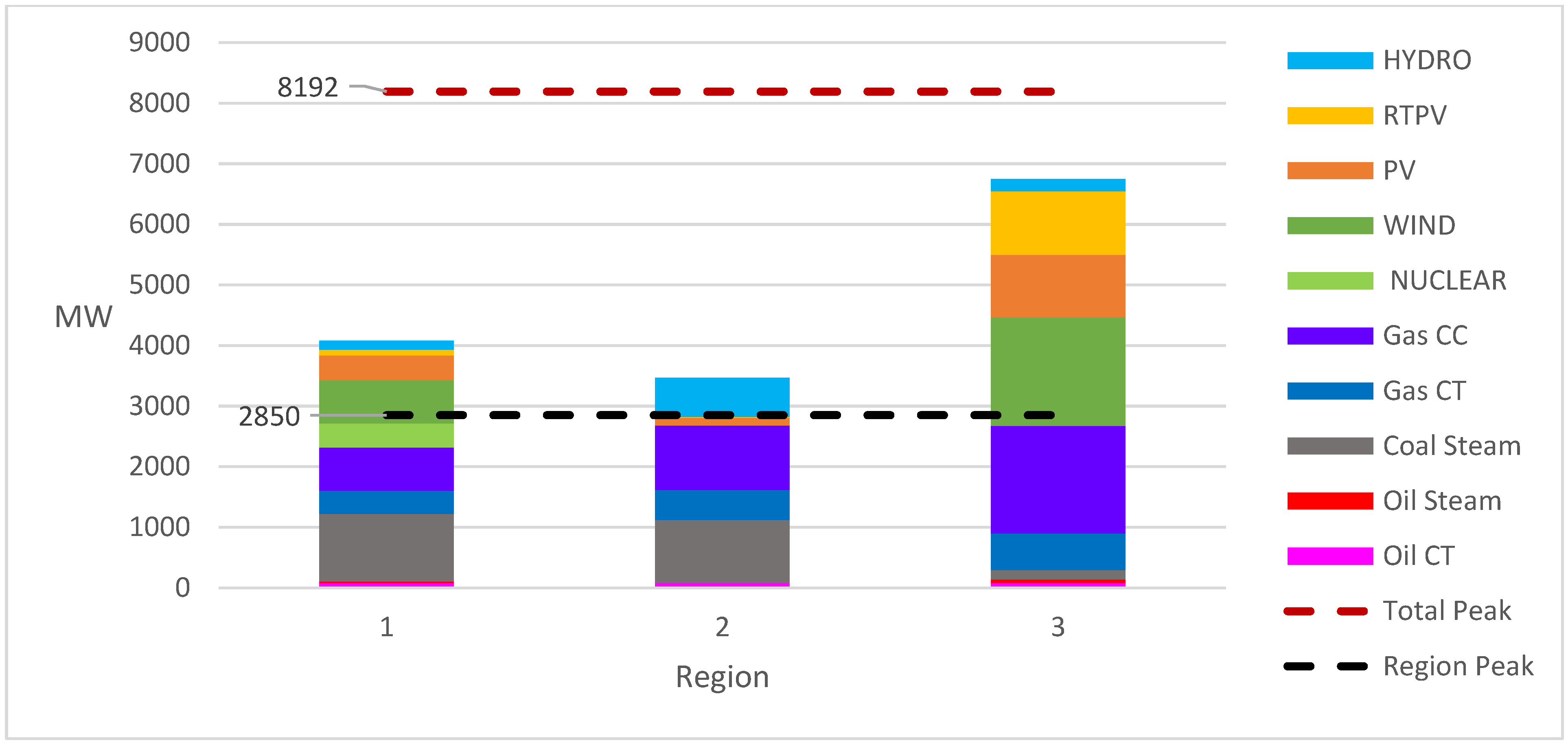As a reference, we employed the existing renewable portfolio standards (RPSs), which prescribe the minimum renewable energy generation for California, Nevada, and Arizona, at 33%, 25%, and 15%, respectively [48]. In the RTS-GMLC, the peak power is about 8.2 GW, and the total conventional generation fleet’s capacity is close to 9.1 GW. Traditional generation is categorized into groups that aggregate units with the same capacity, fuel, and constraint characteristics. The VRE is composed of 1.55 GW of utility-scale solar photovoltaics (PV), 1.16 GW of rooftop solar photovoltaics (RTPV), and 2.51 GW wind. Figure 1 summarizes the generation capacity of the system, with a column for every region, and the height of each column illustrates the capacity in MW. In this figure, every column is composed of stacked sections representing the penetration per technology, as indicated by the legend on the right of the figure, with the fuels and technologies stacked in the order shown in the legend. Note that the proportion of generation is different in every region: Region 1 is the only one displaying nuclear generation; Region 2 shows no wind generation; and most of the VRE is in Regions 1 and 3. The lower dashed line shows the peak demand per region, and the upper dashed line shows the total system peak demand. The constraint characteristics of the conventional generation fleet in this dataset include ramp rate (MW/min), start time (h), shutdown time (h), minimum up- and down-time (h), and start-up heat (MMBtu). Refer to “

Table A1. Generator data summary of the characteristics of the thermal fleet in the RTS-GMLC dataset.

Group	Max (MW)	Min Dispatch (MW)	Min On (h)	Min Off (h)	Hot Up Time (h)	Warm Up Time (h)	Cold Up Time (h)	Hot Start Heat (MMBtu)	Warm Start Heat (MMBtu)	Cold Start Heat (MMBtu)	Raise Ramp Rate (MW/min)	Lower Ramp Rate (MW/min)
U20 Oil CT	20	8	2.2	2.2	0.25	0.75	1	0.005	0.005	0.005	3	3
U76 Coal	76	30	8	4	3	10	12	3.379	4.861	5.285	2	2
U355 Gas CC	355	170	8	4.5	0.5	1	2	3.197	4.536	7.215	4.14	4.14
U55 Gas CT	55	22	1	1	0	0	1	0.038	0.044	0.068	3.7	3.7
U12 Oil ST	12	5	4	2	2	4	12	0.453	1.123	1.457	1	1
U155 Coal	155	62	8	8	3	11	60	6.892	7.438	10.778	3	3
U400 Nuclear	400	396	24	48	9999 *	9999 *	9999 *	9.999 *	0	78.978	20	20
U350 Coal	350	140	24	48	8	12	96	9.768	10.114	17.384	4	4

* The number 9999 flags the nuclear generator as always ON and dispatching at or near install capacity limits.

 Appendix A” for a summary of the characteristics of the thermal generator in the RTS-GMLC dataset.

3.1. Commitment Decisions and Multicycle Rolling Planning Horizons

The constraint parameters of conventional generation in the RTS-GMLC lead to the selection of the modeling cycles. Refer to

Table 2. Key details that describe the multicycle rolling horizon modeling implemented in this study.

Cycle	Horizon	Time Step	Look-Ahead	Commitment	Start-Up Time	Decision Time
SC	24 h	60 min	6 d (144 h)			108 h
WA	24 h	60 min	6 d (144 h)	Steam units	96 > t > 60 h	108 h
DA	24 h	60 min	1 d (24 h)	Steams units	t = 12 h	12 h
4AH	4 h	60 min	1/2 d 12 h	Combined Cycle	t = 2 h	4 h
AH	1 h	15 min	1/8 d 3 h	Combustion Turbines	t < =1	1 h
RT	15 min	5 min	45 min			15 min

for a summary of the key information that defines the multicycle rolling horizon and the corresponding commitment decisions. The slow-start coal units have start-up times of 96 h and 60 h, and therefore fit into a weekly decision cycle, which we call week ahead (WA). Nuclear generators are always committed in the WA, since their startup time is very long. Some coal and oil units have a 12 h start-up time, and consequently these units are committed in the day ahead (DA) cycle. Natural gas combined cycle units have a start-up time of 2 h, and therefore fit into a four-hour ahead (4HA) decision cycle. Natural gas combustion turbines have a start-up time of 1 h, and therefore are committed in the hour ahead (HA) cycle. Finally, hydro and VRE generators (PV, RTPV, and wind groups) operate in the real-time (RT) cycle, which is the trading hour. Forecasts for load and VRE generation are used in each cycle’s commitment optimization. Those units with short startup times are selected and planned for in each optimization cycle, but are not irrevocably committed until necessary.

The previous discussion of the commitment timeframe provides the basis for a multicycle rolling horizon model. In PSO, multiple decision horizons are used to mimic the multiple timeframes used to commit units. The first cycle is called a system cycle (SC), or security analysis, and it approximates the transmission network’s power flow and sets a preliminary schedule that is sufficient to ensure reliability. The time resolution in the SC cycle is hourly for every day, and preliminary decisions are made more than 108 h (4.5 days) in advance. The next horizon is what will hereafter be called the week ahead (WA) cycle, in which slow coal units (start-up time 60 to 96 h) are committed; decisions here are made using data with an hourly time resolution and are completed 108 h (4.5 days) in advance. The next cycle is the DA cycle, which uses hourly data and commits steam units with a start-up time of 12 h. The next decision cycle is the 4HA cycle, which commits CC generators with a two-hour start-up time. Decisions are finalized for these units four hours in advance. The last decision cycle is the HA cycle, which commits CT units with a start-up time of one hour; decisions are finalized for these units one hour in advance. The final layer in the multi-cycle model is the RT cycle, in which the VRE is incorporated and the rest of the generators are dispatched. The schedule is finalized 15 min in advance, and RT decisions are made every 15 min.

Figure 2 presents the rolling horizon multicycle model described above and implemented in PSO. Each of the decision cycles mentioned is represented in the six sets of horizontal bars shown in the figure, starting with the longest lead-time cycles on the top and moving downwards toward RT. For example, the SC cycle is represented by the top set of two horizontal bars, which represent the SC decision cycle over two successive horizons. The gray segments of these bars represent a look-ahead period of six additional days for which the predicted load is taken into consideration by PSO when committing units. Thus, the commitment of long-start units takes into account predicted future conditions. The green segments on the left end of these lines are broken into 24 hourly periods which are represented by the smaller green blocks indicating the hourly resolution of the data and forecasted load in the SC commitment. The look-ahead for each cycle ensures that each planning horizon’s decisions take into consideration the conditions expected in the following time periods. For example, if the load forecast indicates a large change in load at the beginning of the next period, then the units committed must be able to meet that load change. The WA, DA and 4HA cycles each use hourly resolution data, with look-ahead periods of 6 days, 1 day, and 12 h, respectively (see Figure 2). The HA cycle employs a time resolution of 15 min with a 4 h look-ahead period. Finally, the RT cycle has data with a resolution of 5 min with a 45 min look-ahead period; thus, the dispatch takes into consideration the conditions expected in the following 45 min.

In its current formulation, the RTS-GMLC employs hourly time resolution data for any planning cycle prior to the day of operation, such as the DA cycle, and 5 min data for cycles within the day of operation, such as the HA and the RT cycles. Hourly resolution forecast data for the load and VRE were used in the SC, WA, and DA decision cycles, and the actual conditions (RT) were used when committing units in the 4HA, HA, and RT cycles. In PSO, this collection of different cycles is referred to as a multicycle rolling horizon model. For example, the SA cycle is run to define an initial commitment schedule that is sufficient to ensure reliability. For the RTS-GMLC, the SA cycle confirms that nuclear generation is committed and ensures there is sufficient generation available to guarantee reliability. Next, the WA cycle commits slow start units (greater than 12 h start time), followed by the DA cycle, where units requiring greater than 2 and less than 12 h are committed. Next, the 4HA cycle commits CC units with 2 h start-up times, and then the HA cycle for the 1 h start-up CTs. Each of these commitment cycles is executed with the look-ahead periods mentioned previously to ensure awareness of the upcoming load conditions that must be met, so that generation is able to ramp up and meet load changes from one horizon to the next. As the model proceeds with simulating system operation over a specific time period (one-week periods were used in this work, but it could apply to a full year or longer), each of these decision horizons is considered in sequence.

3.2. EV Modeling

One way in which our model is different from the original RTS-GMLC is the introduction of EVs. EV penetration is defined here as the percentage of EVs in the LDV fleet. Because the character of the three regions in the RTS-GMLC is based upon generators in LADWP, NEV, and APS, the number of EVs per region and the EV load per region are derived from an estimation of the vehicles in the LADWP, NEV, and APS balancing areas. Projecting 10%, 20% and 30% of LDVs in each region are EVs, the estimated number of EVs is presented in

Table 3. EV penetration in thousands of vehicles as a percentage of LDVs and of the annual system load, and the number of vehicles assumed in each region.

EV Penetration LDV (% Energy)	Region 1	Region 2	Region 3	Total
10% (1%)	96.9	76.2	197	~400
20% (2%)	193.8	152.4	394	~700
30% (3%)	290.7	228.6	591	~1000

. These penetration levels of EVs correspond very closely to 1%, 2%, and 3% of the energy served in each region, as shown in the first (left-most) column of Table 3. The number of vehicles in each region, in thousands, is shown in columns 2 to 4 of the table, and the total number of vehicles is shown in the column on the right.

The procedure of assigning EVs into each regional node in the RTS-GMLC transmission topology involves splitting the number of EVs based on nodal peak load participation. Thus, nodes with higher load consumption are assumed to have a higher number of EVs.

Table 4. EV nodal distribution at 10% penetration of LDVs in RTS-GMLC Region 1 based on the nodal peak load participation.

Node	Load (MW)	EV
101	108	3672
102	97	3298
103	180	6120
104	74	2516
105	71	2414
106	136	4624
107	125	4250
108	171	5814
109	175	5950
110	195	6630
113	265	9010
114	194	6596
115	317	10,778
116	100	3400
118	333	11,322
119	181	6154
120	128	4352

illustrates the EV distribution by a node at 10% for Region 1, which has a total of 96.9 thousand vehicles. In Table 4, the first column represents the nodes in Region 1, the second column is the load during peak operation, and the third column is the number of EVs in that node.. For example, node 118 shows a larger portion of load consumption and therefore a greater number of EVs. Thus, the higher the load participation factor, the higher the number of EVs.

EV charging data from the EV Project reported by Idaho National Laboratory, including initial and final state of charge [49] and EV charging availability [50], were fundamental to the creation of the statistical models of uncoordinated and coordinated EV charging, which are scalable and suitable for implementation in a PCM [37]. In the uncoordinated scenario, charging occurs at the convenience of EV owners. The load due to uncoordinated charging is implemented with a Monte Carlo technique that uses the charger type, battery capacity, availability for charging, and battery beginning and ending states-of-charge in the EV fleet. Coordinated charging is modeled using an “aggregator”, wherein EV charging is scheduled to minimize operating costs while meeting the daily charging requirements, as subject to battery capacity and charging constraints due to EV availability and states-of-charge. When modeling coordinated charging, to include the effects of the EV load on the electricity price, it was shown that the EVs should be represented as a controllable load, with constraints, with the PCM; refer to [37] for a detailed description of these models.

Coordinated EV charging is represented as an energy-limited (EL) resource in PSO. To meet the expected charging load, PSO allocates the EV’s charging energy (MWh) in the DA cycle, within a time window of 24 h. This process is constrained within a time series with the maximum energy dispatch allowed for the next day, which is a function of the number of vehicles plugged in and their charger capacity per time (vehicle charging availability derived from EV Project). To expand the EV charging plan into consecutive intraday cycles, those with a solution time smaller than the time window of 24 h, such as DA and 4HA, must be used to hold the dispatch of the DA cycle, the process of which is equivalent to a non-recourse decision, but for dispatch purposes. The PCM cannot allocate charging cycles with an optimization window of less than 24 h. Thus, the PSO can include EV charging as part of the system plan in all of the cycles (SA, WA, DA, 4HA, HA, and RT), dispatching the EV that minimizes the system’s operation cost.

3.3. Weeks of Analysis

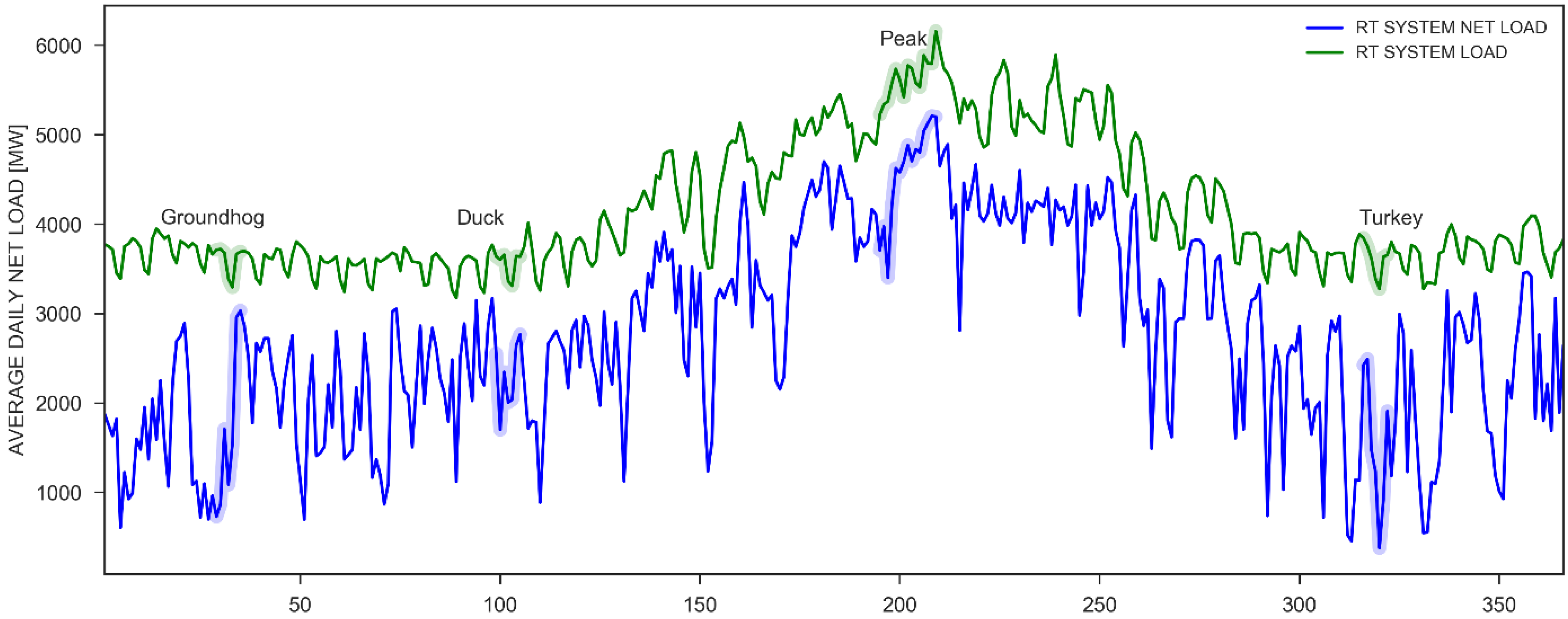
Stress during power system operation, i.e., high LMPs and low reserve margins, depends on several factors including the number of conventional generators online and the load profile, both of which vary throughout the year. This study explores the impact of EVs during some key weeks of the year when stress is expected—some during the winter and spring (off-peak seasons) when VRE is high, but load is not, and some during the summer (on-peak season). The weeks selected were based on overgeneration during the off-peak season, whereas during the on-peak season they included the days of maximum annual peak load and the day with the most significant ramp. Figure 3 shows the monthly distribution of hourly net load (the net load is defined as the load minus VRE) in the RTS-GMLC using a boxplot, representing the 5th and 95th quantiles in the bounds and the 25th, 50th and 75th quantiles in the boxes. In this figure, the only two months without an hourly net load falling below zero are July and August. Figure 4 illustrates the daily average load and net load for each day of the year. The difference between the lines on this plot indicate the daily average VRE. These figures show that the net load is lower in the winter months and higher in the summer months due to the peak loads being driving by cooling loads in the summer.

The weeks analyzed during the low-load months are:

• Wednesday 29 January 2020 to Tuesday 4 February 2020 (Referred to as “Groundhog week”, since Groundhog Day in the U.S. is on Sunday 2 February 2020);
• Wednesday 8 April 2020 to Tuesday 14 April 2020 (Referred to as “Duck week” since the load and VRE generation produce a net load curve that is often called the “duck curve”, and is of significance in the western U.S.);
• Wednesday 11 November 2020 to Tuesday 17 November 2020 (called “Turkey week” since it is near the Thanksgiving holiday in the U.S.).

The weeks analyzed during the summer operation are:

• Monday 13 July 2020 to Sunday 19 July 2020 (the most significant daily ramp is on Thursday 16 July 2020 with value of 4600 MW);
• Wednesday 22 July 2020 to Tuesday 28 July 2020 (peak load is on Monday 27 July 2020).

Due to the proximity of the summer weeks, the model is run for two consecutive weeks from Monday 13 July 2020 to Tuesday 28 July 2020.

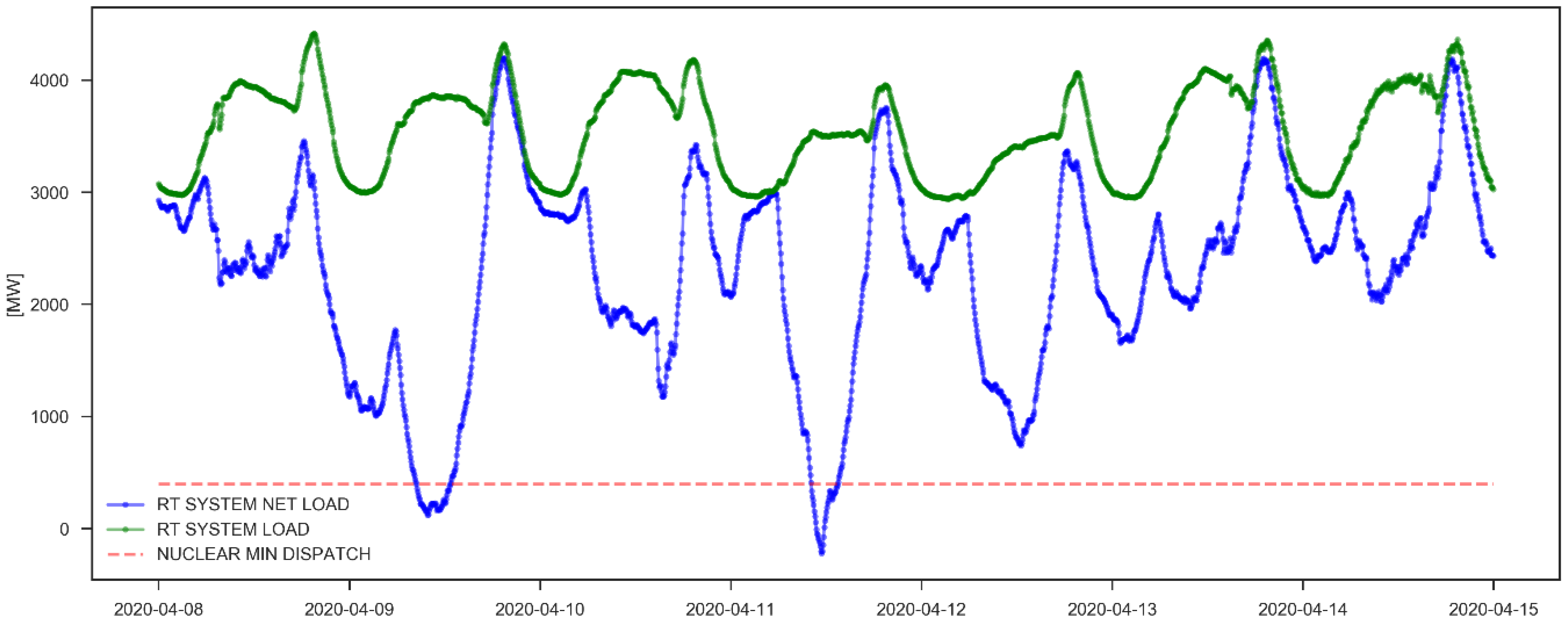
Figure 5 shows the load (solid green), net load (solid blue), and minimum dispatch (dotted red) of nuclear generation (vertical axis in MW) during Duck week. Notice the two red boxes highlighting two days (9 April 2020 and 11 April 2020) on which the high penetration of VRE pushes the net load below the minimum dispatch of nuclear, and even into negative values. The expectation is that a net load below the minimum dispatch of nuclear power will result in the curtailment of VRE.

4. PCM Results and Metrics

Before describing the base case scenario and cases with EVs, it is necessary to describe the PCM results regarding system operation cost, marginal electricity cost and aggregated generation dispatch stack to serve the demand, as well as key reliability metrics. The system operation cost is the sum of the expenditures and fuel costs related to running the RTS-GMLC system’s generators. The fuel cost has different components: the fuel expended during the startup, the fuel used to keep the machine running regardless of the level of generation, and the variable fuel cost derived from the incremental heat rate curve, which changes according to the production of the machines. The other variable costs are small compared with the fuel expenditures and are neglected. To keep the operation cost as low as possible, it is necessary to use the most fuel-efficient power plant first, and only operate the least efficient if it is strictly needed. The different levels of EVs allow us to explore changes in this system with a new load, the influence of which changes according to the size of the EV fleet.

The marginal electricity cost is the price paid for the last unit energy purchased. Since transmission constraints can exist between different areas within a power system, including the areas in the RTS-GMLC, the marginal cost of electricity can vary by location, and is thus called the locational marginal price. The marginal generator, which supplies the next energy unit, sets this electricity cost. Therefore, if the marginal generator does not use fuel to generate electricity, that is, uses only solar or wind, the LMP is zero. Each generator’s revenue is the product of the electricity cost (LMP) times the energy produced by the generator. The cost of charging the EVs is the difference between the production cost with a given penetration of EVs minus the production cost of running the system with no EVs.

Additionally, we explore the operational curtailment, power not delivered from VRE due to constraints in the conventional fleet, and demand and reserves not served as reliability metrics. These reliability metrics determine the system’s flexibility in the face of changes in the net load, resulting from either changes in the load or instantaneous VRE penetration.

5. Cases Examined

A total of 28 cases were examined through the use of the PCM for the weeks described earlier. For each week, EV penetration levels of 0% (base case), 10%, 20%, and 30% were considered. When EV loads were introduced into the RTS-GMLC, they were analyzed twice: once assuming uncoordinated charging and once with coordinated charging. A summary of the cases examined is presented in

Table 5. Enumeration of the cases considered in the analysis of the effects of EV charging in the RTS-GMLC.

		Charging Strategy
Week	Base Case	Uncoordinated	Coordinated
29 January–4 February (Groundhog)	0%	10, 20, 30%	10, 20, 30%
8–14 April (Duck)	0%	10, 20, 30%	10, 20, 30%
13–28 July (Peak)	0%	10, 20, 30%	10, 20, 30%
11–27 November (Turkey)	0%	10, 20, 30%	10, 20, 30%

. The lefthand column describes the week, and the numbers in the subsequent columns show the EV penetration level in percent of the LDV fleet. Remember that these EV penetration levels correspond very closely to 1%, 2% and 3% of the overall system total load.

The base case scenarios provide results for operating the RTS-GMLC with no EVs and typical electricity prices. These results are useful to gain insights into the normal operation of the RTS-GMLC and to ensure that the PCM is producing a rational solution for commitment and dispatch (i.e., under normal conditions, load should be met by generation without violating reserve margins). The four different weeks, three EV penetration scenarios, two charging strategies, and four base scenarios with no EV led to a total of 28 runs of the PCM. Comparing the results of the different EV penetration scenarios allow us to analyze the effects on system operation under different system conditions during the annual peak load and off-peak weeks during which the load is low and VRE is high (overgeneration). In the sections to follow, we present results for all the cases analyzed, with a focus on the results for Duck week (April) and the Peak (summer) weeks to determine differences in production costs, LMPs, the generation stacks, VRE curtailment, and reliability metrics of unserved energy (load shed) and reserve shortages. The results for the base case without EVs will be presented first, followed by the cases with EVs.

The most relevant results from these cases will be presented.

6. Results without EVs

This section shows the production costs, electricity prices, generation mix, and reliability metrics for the RTS-GMLC base case without EVs. The production costs will be presented first along with some reliability indicators, followed by exploring the generation mix required to serve the demand, followed by the electricity prices and VRE curtailments.

6.1. Production Costs and Reliability Metrics

The average production costs for the RTS-GMLC base case are shown in the second column of

Table 6. Summary of production costs and reliability metrics for the RTS-GMLC base case with no EVs.

Week	Average Daily Production Cost (Million USD)	Peak Load (MW)	Unserved Energy (MWh)	Reserve Shortages (MW)
Groundhog	0.709	4468	0	0
Duck	0.744	4484	0	0
Peak	1.963	8036	0	0
Turkey	0.548	4780	0	0

for the weeks of analysis listed in the first column. Notice that the average production cost in the peak season is more than double that in the other weeks of the study, while the peak load is about double that of the rest of the year. The reliability metrics of interest are the unserved energy (load shed) and reserve shortages. If there are problems in the unit commitment and economic dispatch solutions of the PCM, and the load cannot be met with generation, the result is unserved energy. The PCM seeks to minimize the operation cost. In doing so, the PCM is set up to avoid load shed by assigning a high cost, i.e., a penalty, if load is shed. Thus, in minimizing the production cost, it is advantageous to avoid high penalties for unserved energy. As can be seen in Table 6, for the base case setup with no EVs, there is no load shed, and consequently the production costs result from the costs for generation unit startup and marginal costs of operation. Reserve shortages are used to indicate when the PCM solution is not able to maintain the necessary reserve margin. The reserve margin used in the RTS-GMLC model is 3% of the load served during any hour for spinning reserve, and on average 2% of the load for non-spinning reserves and flex reserves. When the reserves allocated in the RTS-GMLC fall below what is required, then the shortfall is reported as a shortfall in the capacity in MW. As shown in Table 6, there are no reserve shortages in the base case. Together, these reliability metrics show that the RTS-GMLC base case with no EVs results in a rational dispatch, and that the load can be met with existing generation and reserve margins.

6.2. Generation Stack

6.2.1. Generation Stack during the April Week (Duck Curve)

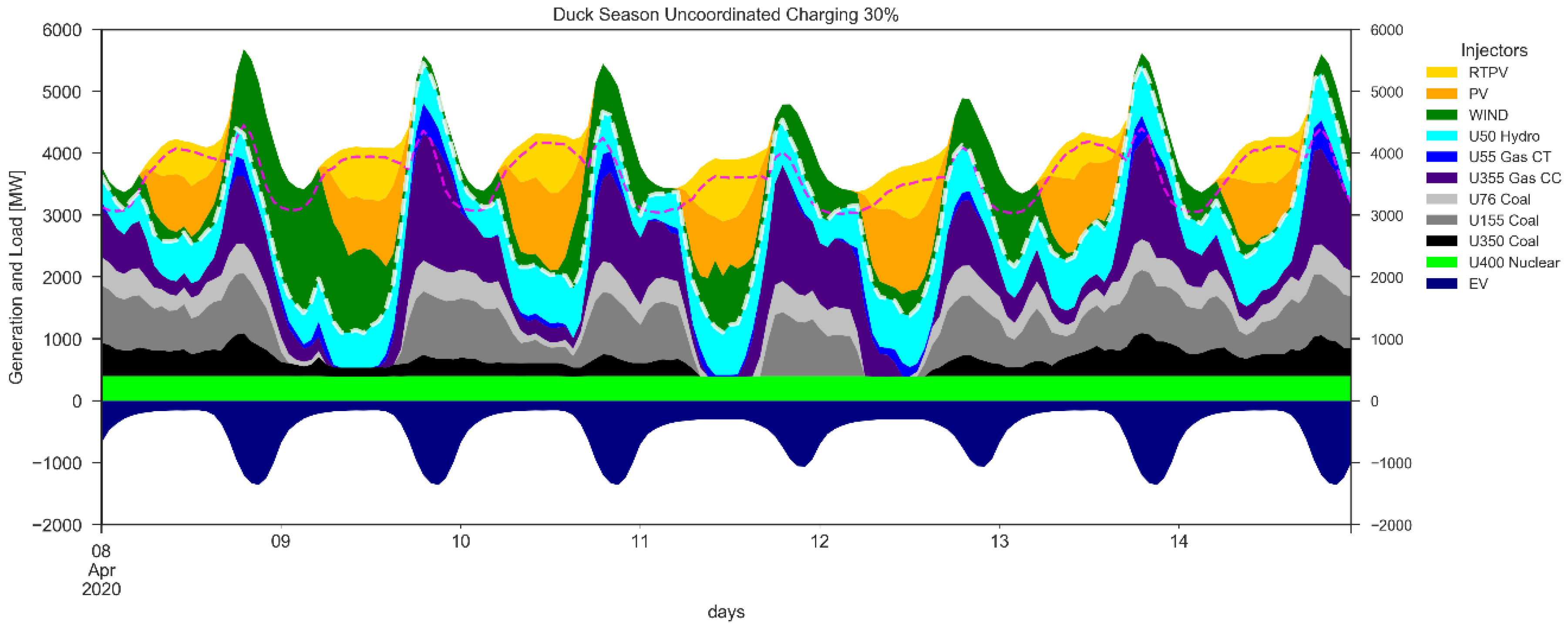
A generation stack illustrates the generation resource used to serve the demand. For the RTS-GMLC base case with no EVs, the “generation stack” for the duck week (April) is shown in Figure 6. The vertical axis on this plot shows the generation and load in MW, and the horizontal axis shows the days of the week. Shown on the plot is the load (magenta dashed line), net load (white dashed line), and generation used to meet the load. Note the “net load” is defined here as the load minus VRE. The generation plotted in the stack is identified in the legend. Starting at the bottom, the legend shows the EV load in navy blue; note that there are no EVs shown in the stack for this base case (EV load will be shown as a negative). Next in the generation stack is nuclear generation, here illustrated in green, with a dispatch that does not vary with time. Above nuclear in the stack are three types of coal steam units: 350 MW units (black), a 155 MW unit (gray) and 76 MW units (silver). The next two in the stack are a natural gas combined cycle, NG-CC (indigo), and a natural gas combustion turbine, NG-CT (blue), with capacities of 355 MW and 55 MW, respectively. Next on the stack is a 50 MW hydropower unit (cyan), which is topped by the VRE generation: wind (green), utility-scale PV (orange) and roof-top PV, RTPV (gold). Looking at the generation stack across this week in April, there are days in which VRE plus hydro supplies most of the power during daylight hours, for example on 9, 11, and 12 April. As can be seen, during the middle of the day when VRE generation is high, their production flattens out as the resources are curtailed to permit the nuclear generation to maintain its steady output (in the RTS-GMLC, the nuclear generation is not allowed to ramp). During each day shown, in the late afternoon when RTPV and PV generation drops, and the fossil generators (natural gas and coal) must increase their output (ramp) to supply the daily peak demand in the evening hours and much of the overnight load. During this week, which is representative of weeks in the spring in the Southwest U.S., the flexible CC and CT units are crucial in following the net load, and what flexibility that does exist in the smaller coal units is also utilized.

6.2.2. Generation Stack during the July Weeks (Peak)

Figure 7 shows the generation stack during the peak weeks in July. The daily peak load occurs during the afternoon (2 p.m.) on 27 July. RTPV and PV generators are available at the peak, thus reducing the peak net load (white dashed line) substantially to 6524 MW. In July, the coal steam units (black to silver) tend to fluctuate less from day to day than the other weeks analyzed. Focusing on 15 July, we can see a large contribution from the wind resource, further reducing the peak net load, but this is not common during these weeks in July (this is consistent with wind resources in the Southwest U.S.). On each of the days analyzed, the flexibility of the natural gas generators (CC and CT) is used to fill the gap between the net load and the less flexible coal and nuclear generators by ramping up and down each day. On days with significant solar and wind generation (13–15 July), the flexibility of the CC and CT units is key to meeting the net load variations. Compared to the spring “Duck” week, the commitment and dispatch are much more consistent, and more like those in systems with low VRE penetration.

6.3. Locational Marginal Price (LMP)

This section describes the average LMP in the system as the load-weighted LMP for the whole network.

Table 7. Load-weighted average LMP (USD/MWh) over all nodes in the RTS-GMLC without EVs.

Week	Average LMP (USD/MWh)	Average Load (MW)
Groundhog	14.85	3682
Duck	17.86	3641
Peak	25.12	5821
Turkey	15.09	3684

presents the weekly average LMP in each week considered. The LMP was tabulated as the average load-weighted LMP on each node in the RTS-GMLC system. Note that the highest LMP occurs during the peak season when the load is the highest. The LMP during the peak weeks is about 60% higher than during the off-peak weeks.

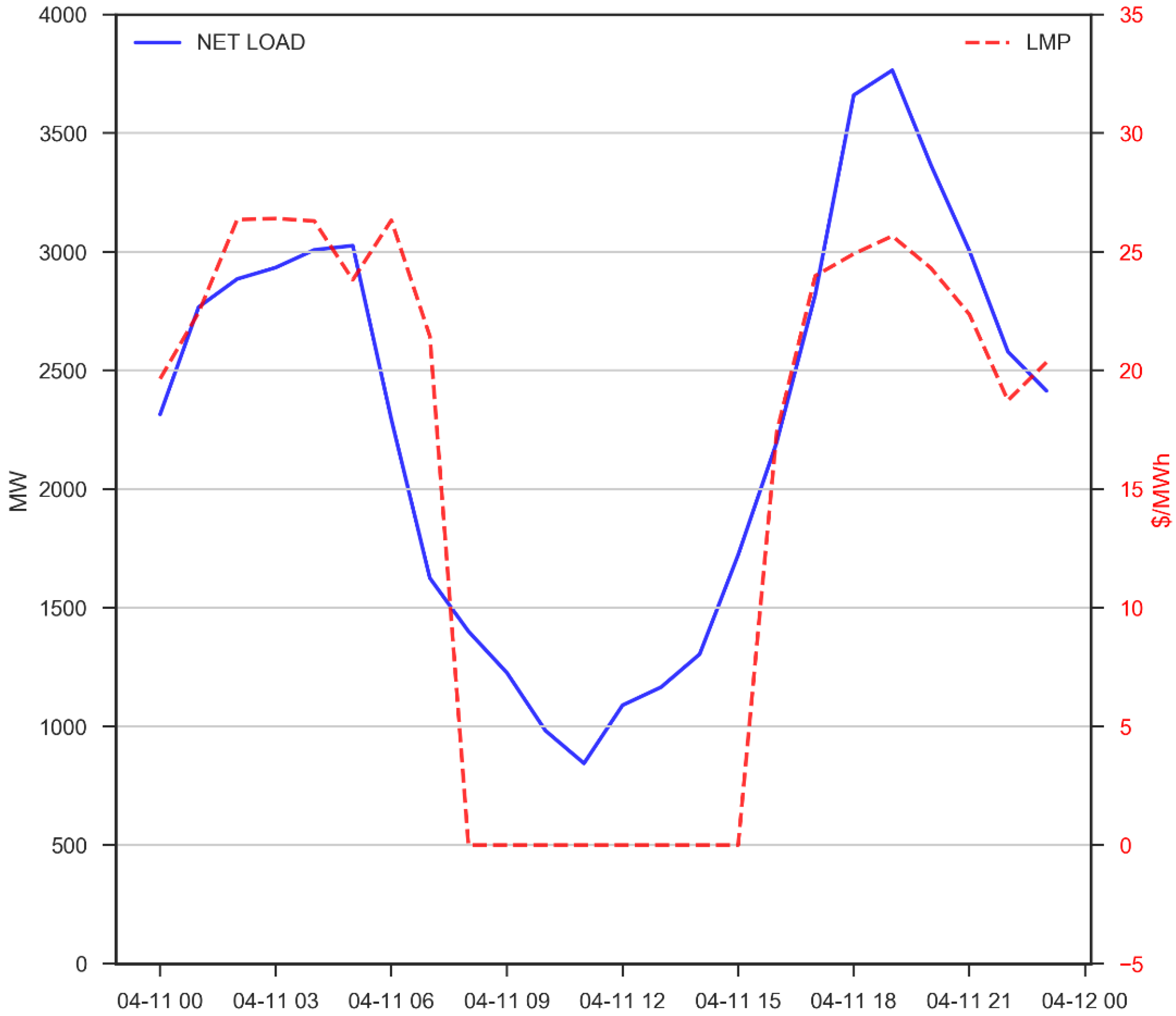
An example of the LMP variation during a typical day (11 April) during the Duck week without any EVs is shown in Figure 8. The system’s 5 min net load in MW is indicated by the solid line and refers to the scale on the left, and the system load-averaged LMP at a 5 min resolution is indicated by the dashed red line and refers to the scale on the right in USD/MWh. The LMP follows the trend of the net load since the price of the marginal generator declines as the net load declines.

The net load curve in Figure 8 shows a large dip in the middle of the day, and steep ramps in the morning and evening, which are characteristic of the Duck curve. Running the PCM PSO for the Duck week leads to an LMP that hovers at between USD 20 and 25 per MWh in the nighttime hours, and drops to zero during the day when the net load is very low. During zero-LMP hours, solar generation is the main marginal resource. These results are consistent with operational experience during periods of high VRE and overgeneration.

6.4. VRE Curtailments

Because the net load can at times fall below the minimum dispatch level, it may be necessary to curtail the VRE. Referring to Figure 5, at midday on 11 April, the minimum net load falls below the minimum dispatch of nuclear generation (see the blue net load line, and the horizontal red dashed line). After honoring the system constraints, including generator minimum dispatch level, the net load on 11 April after VRE curtailment is shown by the blue line in Figure 8. 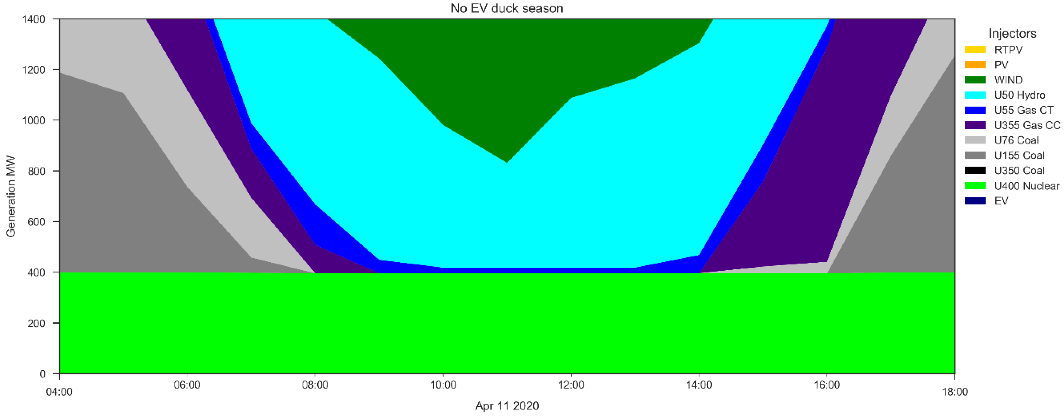Figure 9 shows a zoomed-in view of the bottom of the generation stack, below 1400 MW, for 11 April between 4:00 and 18:00 from Figure 6. The coal and CC units are cycled off, subject to their minimum time-off fulfillments (commitment parameter) of eight hours (U155 Coal (gray)), four hours (U76 Coal (silver)), and four and a half hours (U355 Gas CC (indigo)). Additionally, in Figure 9 between 10:00 and 13:00, a CT unit is shown as running at its minimum dispatch of 22 MW. The nuclear generation remains constant, while the hydro and natural gas CTs operate at their minimum dispatch levels until later in the afternoon when the PV decreases. During the window of time from 9:00 to 17:00, there is VRE curtailment of 4042 MWh.

Table 8. VRE curtailments expressed as a percentage of total weekly VRE production for each of the weeks analyzed for the base case with no EVs.

	VRE Curtailment
Week	Wind	PV	RTPV
Groundhog	9%	18%	5%
Duck	4%	12%	1%
Peak	1%	0%	0%
Turkey	7%	14%	2%

summarizes the total curtailment during each of the weeks analyzed for the base case with no EVs. The percentage of VRE curtailment reported is the amount of energy produced by VRE that is not used. Focusing on the Duck week where VRE curtailments are moderate during the off-peak season, the RTPV curtailment is the smallest, at less than 1%; wind curtailment is less than 4%, and PV curtailment is largest at 12%. During the peak weeks analyzed with no EV, the curtailment of PV and RTP was zero, while it was approximately 1% for wind. Curtailment is greater during the off-peak weeks because the load is relatively low, while VRE production can be high.

7. Results for Cases with EVs

This section presents the results from running the PCM for the weeks of interest when employing either uncoordinated or coordinated charging strategies for EVs. These results will be compared with the base case RTS-GMLC and between themselves.

7.1. System Operation Cost

Figure 10 presents the daily average operation cost, in millions of USD, for all weeks analyzed and for all scenarios. The four-column groupings along the horizontal axis represent the levels of EV penetration and charging approach, from no EVs on the left up to 30% on the right. Inside each group of columns, the colors (order) represent the different weeks of analysis, starting from early in the year (leftmost column) to late in the year (rightmost column). The operating cost (start-up and operational fuel costs) is proportional to the net load served for the conventional generation fleet, and ranges from USD 0.5 M to nearly USD 2.5 M. In the RTS-GMLC, the net load is highest in the summer peak load months (annual peak in July; see Figure 4) and lowest in the off-peak winter months (lowest monthly peak in November; see Figure 4). Therefore, as shown in Figure 10, the operating cost is higher during the summer (third—orange columns) than in the non-peak seasons, and more than three times higher if one compares days in July (peak) and November (turkey) at every penetration level. Regardless of the level of EV penetration or week, coordinated charging results in a lower operating cost than uncoordinated charging. The savings achieved in operating cost when using coordinated charging are consistently 1% during the summer peak weeks. The savings, however, ranged from 4% to 8% during the other weeks. The percent savings are more significant at 10% EV penetration than 20% or 30% EV penetration, due to lower fuel expenditure and less generation being committed to cover the additional power consumption due to EVs. In summer, EV represents a smaller proportion of the net load, and the savings are lower.

7.2. Cost to Charge EVs

The cost due to EV charging is determined by taking the difference between the production cost with a given penetration of EVs and the production cost of running the system with no EVs. Figure 11 presents the average daily EV charging cost per vehicle for each of the scenarios. In Figure 11, the charging cost is shown on the vertical axis, while the horizontal axis illustrates the levels of EV penetration and charging approach, following the convention of Figure 10. Note that the charging costs range from USD 0.05 to USD 0.25 per day, which is consistent with the energy requirements for the battery size and the charging requirements of the LDVs assumed in this model (equivalent to a daily usage of about ~10 kWh per vehicle, equivalent to ~30 miles a day). No transmission use payments are considered, nor are the costs of distribution to end-users or any other costs. For the peak week, when comparing coordinated and uncoordinated charging costs for all three penetration levels, the cost goes down by 10% percent. This happens because the coordinated charging approach accommodates EV charging when VRE is available. For the Duck week, the cost reduction elicited by coordinated charging varies from 45% to 24% as the EV penetration increases. The jump in charging cost for coordinated charging from 10% to 20% and 30% EVs is due to the number of fossil generators that must be used to provide power, with an additional generating unit being committed. Overall, the cost of charging EVs is substantially lower when using coordinated charging versus uncoordinated charging.

7.3. Locational Marginal Price (LMP)

Table 9. Weekly average LMP (USD/MWh) occurring over the entire system (RTS-GMLC).

Scenario	Groundhog (USD/MWh)	Turkey (USD/MWh)	Duck (USD/MWh)	Peak (USD/MWh)
NO EV	14.85	15.09	17.86	25.12
10% EV Uncoordinated	16.17	17.34	18.42	25.57
10% EV Coordinated	16.71	16.12	20.48	25.44
20% EV Uncoordinated	16.75	16.35	19.12	25.85
20% EV Coordinated	17.75	17.98	20.48	25.76
30% EV Uncoordinated	17.63	17.86	19.53	26.14
30% EV Coordinated	19.73	18.41	21.10	26.23

shows the weekly average LMP in the RTS-GMLC system for all scenarios. The first column lists the scenarios, followed by columns for every analysis week, ordered from lowest to highest LMP (Groundhog, Turkey, Duck, and Peak). Note that the first row provides the same data as Table 7 and shows the lowest LMP because it has the lowest total demand (no EV charging). The highest LMPs arise at 30% EV penetration due to the higher overall load. For example, at 30% penetration of coordinated EV charging, the average LMP increases by 4% compared to a system with no EV charging. Comparing the LMP of the various scenarios, the uncoordinated cases often have a lower LMP than their coordinated counterparts. Although production costs are lower with coordinated charging, it is not uncommon for the LMP to be higher because the load shifts to times with lower prices, often increasing the low prices during those periods, leading to an overall increase in LMP.

7.4. Generation Stack

This section presents the cumulative generation dispatch for the system, comparing uncoordinated and coordinated charging. The generation stack figures are similar to those shown in Figure 6 and Figure 7. The results shown below refer to an EV penetration rate of 30% of LDVs, corresponding to 1% of the annual energy load.

7.4.1. Generation Stack April Week (Duck Curve) Uncoordinated EV Charging

Figure 12 shows the generation resources used to supply the demand for the case of 30% uncoordinated EV charging. Note that there are two primary differences in this generation stack and the stack shown in Figure 6 for the system with no EVs: (1) the uncoordinated EV charging load is plotted on the negative side of the generation scale (navy blue) and (2) the generation stack includes the generation needed to serve the EV load, so is higher on a daily basis. Shown on the plot in Figure 12 is the load without EVs (magenta dashed line), the net load with EVs (white dashed line), and the generation used to meet the load. Because the EV load for uncoordinated charging peaks every day in the evening, the peak net load exceeds the peak load without EVs on five of the seven days analyzed, with no change on the other two days. Consequently, on some days the dispatch of fossil generation increases during the peak conditions. For example, on 9 April and 13 April, the peak net load exceeds 5000 MW, representing a large increase of 1200 MW (27%) relative to the case with no EVs. Especially on the days when there is nor VRE during the peak hours after sunset, the fossil generation increases output to meet the increased net load.

7.4.2. Generation Stack April Week (Duck Curve) Coordinated EV Charging

Figure 13 presents the case of 30% EV penetration employing coordinated charging. Notice how, in contrast with the previous scenario, coordinated charging shifts this EV load (navy blue on the negative side of the stack) to the middle of the day and takes advantage of the low LMPs resulting from the high VRE or light load during the night. Note that the net load tends to show a morning and evening peak each day (white dashed line). Within the constraints of meeting the daily EV charging load, subject to the constraints of availability for charging and charging requirement, the EV charging aligns with solar power in the middle of the day and wind power during the evening hours. Overall, the peak of the net load served each day is lower than the corresponding peak load without EVs, due to coordinated EV charging aligning better with the VRE. Comparing the shape of the generation stacks in Figure 12 and Figure 13, with coordinated charging, the fossil generators are used less and cycled more to meet the net load.

7.4.3. Generation Stack July Weeks (Peak) Uncoordinated EV Charging

Figure 14 shows the case of 30% uncoordinated EV charging during the peak weeks in July. On two of the days, 16 and 21 July, the peak net load (dashed white line) increases by about 3.8% (300 MW) above the peak load without EVs, shown by the magenta dashed line. On the remaining days, the peak in the net load is equal to or less than the peak load without EVs. On every day, the EV load shifts the peak net load two hours later into the early evening (7 p.m.). Relative to the off-peak weeks, the magnitude of impact on peak load is less during the summer peak weeks, since the peak load is significantly higher.

7.4.4. Generation Stack July Weeks (Peak) Coordinated EV Charging

In Figure 15 is shown the case of 30% coordinated EV charging. Similar to the Duck week (Figure 13), coordinated charging shifts this EV load to the middle of the day, and takes advantage of the low LMPs due to VRE, primarily solar. With coordinated charging, the daily peak net load (white dashed line) is shifted two hours later into the evening relative to the peak load without EVs (magenta dashed line). More importantly, the peak net load is always less than the peak load with uncoordinated charging, and sometimes substantially so. Similar to the Duck week results, the output of the fossil units changes more frequently than with uncoordinated charging.

7.5. VRE Curtailments

We will next look at curtailments of VRE at all penetration levels considered for both charging strategies, and as compared to the case of no EVs. As stated previously (Section 7.2), VRE curtailments are often necessary to keep conventional generation online during low “net load” periods in the middle of the day (to honor generator constraints) and/or to maintain sufficient operating reserves. In the no EV base case, curtailments of VRE are higher during April because of high VRE production and low load (see Table 8).

April Week (Duck) Curtailments

The curtailment of VRE (wind, PV, RTPV) for the Duck week is shown in Figure 16. The curtailment percentage is shown on the vertical axis, and the grouping of bars indicates the magnitude of curtailment for each scenario. The first group of columns regards the case without EV charging (NO EV), followed by the uncoordinated charging scenarios (U10%, U20%, and U30%), and the last three for the coordinated charging scenarios (C10%, C20%, and C30%). This ordering shows that the curtailment is highest in the case without EV charging. Adding EVs in the uncoordinated cases reduces curtailment relative to the base case, due to the additional load. Comparing the three uncoordinated penetration levels, as the EV penetration increases, the curtailment of PV and RTPV decreases. This is due to additional EV load added during hours of PV generation. Wind curtailment, however, increases across the uncoordinated cases because as the EV load increases, additional thermal generation is committed that requires wind production to decrease during the hours where not much charging occurs. For the coordinated charging cases shown in the rightmost set of columns, it is evident that the magnitude of curtailment is lower than for no EVs and for uncoordinated charging. Both wind and solar curtailment decrease with increased EV penetration because the EV load can be scheduled (within availability and charging requirement constraints) to occur during low LMP hours with high VRE production.

Figure 17 shows the VRE curtailments during the peak weeks in July. Note that the vertical scale in this figure is 1/10 of that in Figure 16, and the level of curtailment is smaller in all scenarios as compared to the Duck week. In all cases, the curtailment of PV and RTPV is zero, and the curtailment of wind is lower than 1.3%. The curtailment of WIND starts at 1.0% (NO EV) and increases with uncoordinated charging (U10%, U20%, and U30%). Similar to the Duck week, the increase occurs because additional thermal generation is committed to meet the additional load due to EVs during the on-peak hours, causing wind to be curtailed away from the peak. For the coordinated charging cases (C10%, C20%, and C30%), the wind curtailment decreases with increasing EV penetration, once again because of the ability to move some of the EV charging load to low LMP, high VRE hours. Therefore, coordinated charging reduces wind energy curtailment in July.

8. Discussion

The uncoordinated charging scenarios were established to explore the effects of charging at the convenience of EV users, based upon actual charging habits recorded as part of the EV Project [44], which led to increases in the peak load. Figure 18 shows the uncoordinated EV charging load for 30% EV penetration and LMP for the same day as in Figure 8 (11 April, Duck week). In Figure 18, the uncoordinated charging load is presented with the solid blue line, referring to the vertical axis on the left. The system’s LMP values are depicted in the dashed red line, and refer to the secondary axis on the right in USD/MWh. Figure 18 shows EV charging peaks in the evening, reaching a value greater than 1000 MW during the time when the LMP is high. Consequently, the cost of EV charging is relatively high, and the operation cost is higher.

The results for coordinated charging confirm that when EV charging is scheduled to coincide with low electricity prices, within the constraints of EV availability and charging requirements, the charging costs and system operation cost will be lower. Figure 19 shows the EV charging load profile and LMP for the same day in April as the previous figure. Note that the EV charging is scheduled to occur during the low LMP hours, and that LMPs change in response to additional load being served relative to the no EV and uncoordinated charging cases.

9. Conclusions

This article presented the impacts of EV charging on operation of the RTS-GMLC power system using the PCM PSO. In the base case, the RTS-GMLC model included no EVs. Modeling of EVs considered two charging strategies, uncoordinated and coordinated, and three EV penetration levels: 10%, 20%, and 30% of the light-duty vehicles (equal to 1%, 2% and 3% penetration of the annual energy load). To understand the impacts, the model was applied for representative on-peak and off-peak weeks throughout the year. The findings are presented in terms of power system loads, operation cost, LMPs, EV charging cost, and VRE curtailment, and the impact of the two charging strategies. With regard to the reliability metrics of unserved energy and maintaining reserve margins, the EV charging scenarios led to no increase in unserved energy, and no violation of the reserve margins.

The integration of electric transportation increases the power system load, operation cost, and electricity prices, but the magnitude and character of the effects depend upon the charging strategy. The overall system operation cost under uncoordinated charging is higher, regardless of the level of EV penetration, when compared to coordinated charging. The operation cost is proportional to the net load served by the conventional fleet, and consequently much higher during the peak load weeks in the summer. During the summer weeks, the savings in production costs between coordinated charging and uncoordinated charging are consistently 1% for all three EV penetration scenarios tested. However, during the off-peak weeks when load is lower and VRE production is high, the savings in production costs range from 4% to 8% when using coordinate charging.

EV charging cost was computed by taking the production cost for a scenario with a given EV penetration level and subtracting the cost of running the system with no EVs. The average charging cost per EV follows the same trends as the system operation cost—higher on summer days and lower on winter days, due to the higher LMP, but there are significant differences when considering the charging strategy. At 10% EV penetration (1% in energy penetration) during February (Duck week), the uncoordinated charging cost per vehicle is four times higher than the coordinated charging cost. The lowest savings in charging cost occurred for 30% EVs during the peak weeks in July, because electricity prices are generally high due to high load and LMPs during those weeks.

Regarding the daily system peak load, during off-peak weeks under uncoordinated charging, the peak net load increases with an increase in EV penetration, because peak load and EV charging are coincidental. During a week in April (Duck week), operating under uncoordinated EV charging, the peak load increases as much as 27% at 30% penetration of EVs (3% in energy penetration). However, coordinated EV charging shifts the EV charging load to off-peak hours as much as is possible, within the constraints of the charging requirement and the availability for charging. The result is an increase in the charging during off-peak hours, which is coincident with PV, RTPV, and wind. The net load profile during the day changes under coordinated charging, but the peak load does not increase.

Related to the LMP, the shift of charging to off-peak hours due to coordinated charging increases the LMP simply because the EV load increases during those off-peak hours, and consequently the LMP increases during those hours. During the Peak weeks (July), with 30% penetration of coordinated EV charging, the average LMP increases by 4.4% compared to the system with no EV charging. However, it increases by 33% during a winter week in early February. Note that although the LMP increases, both the operation costs and EV charging costs decrease with coordinated charging versus uncoordinated charging.

Regarding VRE curtailment, coordinated charging reduces the curtailment of PV (by as much as nine times during off-peak season operation for 30% EV penetration) and wind (more than half during the summer operation season for 30% EV penetration) compared to the scenario with no EVs or uncoordinated EV charging. Coordinated charging reduces the curtailment of VRE, mainly because charging can be scheduled at hours of peak PV generation when the LMP is low, which addresses the problem of overgeneration (Duck curve). Therefore, coordinated charging is beneficial to the integration of VRE. To realize this potential for scheduling the charging during low LMP, high VRE hours of operation, it is necessary to have an accurate model of EV availability for charging and charging requirements.