Model Predictive Operation Control of Islanded Microgrids under Nonlinear Conversion Losses of Storage Units

Abstract

This paper proposes a certainty equivalence model predictive control (MPC) approach for the operation of islanded microgrids with a very high share of renewable energy sources. First, to make the MG model more realistic, the conversion losses of the storage units and the conversion losses of the power electronic devices are considered by the quadratic functions in the dynamic of units. Then, to mitigate the effect of errors in the storage units’ state of charge prediction, the conversion loss functions are reformulated by the mixed-integer linear inequality functions and included in the proposed scheme. Finally, the effectiveness of the proposed certainty MPC is verified by a numerical case study.

1. Introduction

Electric power systems have played a pivotal role in technological advances, infrastructure development, and economic growth since their invention [1]. However, conventional power systems typically use fossil fuels (for example, coal, natural gas, or oil) and nuclear and hydropower plants [2]. Unfortunately, the performance of most of them leads to a significant increase in greenhouse gas emissions. Hence, in recent years, researchers have been encouraged to reduce greenhouse gas emissions and fossil fuel consumption in power systems. One of the most effective ways to reduce greenhouse gas emissions is by replacing conventional generators with Renewable Energy Sources (RES) [3]—for example, Photo-Voltaic (PV) power plants or Wind Turbines (WT). Furthermore, to facilitate the integration of a sizeable number of renewable Distributed Generation (DG) units, the concept of microgrids (MGs) has become increasingly popular [4,5].

A microgrid is a small-scale power system, generally consisting of conventional generators, RESs, Energy Storage Sources (ESSs), and loads interconnected by transmission lines [6,7,8]. In general, MGs can be typically operated in grid-connected or island mode. Recently, the MG control system has been standardized into three layers [7]. The inner loop is called Primary Control (PC), and it provides the references for the DG’s DC-AC power converters. The PC is decentralized to establish the desired sharing of power among DGs while preserving the MG stability by employing a droop control term. This layer typically operates on a fast timescale (in the range of tens of milliseconds to seconds). Then, because inverter-based DGs have no inertia, a Secondary Control (SC) layer is needed to compensate for the frequency and voltage deviations introduced by the PC’s droop control terms and generally operates on a timescale from seconds to minutes. Finally, the operation control is designed to optimize the operation of the MGs by providing power setpoints to the lower control layers. The operation control typically operates on a timescale from minutes to fractions of hours. For this task, model predictive control (MPC) approaches are considered a good choice as they allow us to include constraints on the units explicitly and evaluate the system dynamics. This work mainly focuses on the optimal operation of microgrids with a high share of renewable sources.

1.1. Literature Review

Several control schemes have been reported for the operation of islanded MGs. According to how they handle uncertainties, these approaches can be categorized as: (i) certainty equivalence, wherein a forecast in the form of the mean value is fully reliable; (ii) worst-case, where no possibility information is presumed; (iii) risk-neutral stochastic, where a forecast probability distribution is thoroughly reliable, and (iv) risk-averse, where uncertainties in the forecast probability distribution are considered.

In this context, a two-stage operation control algorithm is recorded in [9], which includes a schedule and a dispatch layer. To dispatch generators of islanded MGs, an energy management approach is proposed in [10] by adapting the power setpoints and droop gains of the units. Furthermore, a method is provided in [11] to schedule islanded MGs. However, refs. [9,10,11] do not allow us to limit infeed from RES. By using genetic algorithms, a day-ahead schedule for MGs is also designed in [12]. Additionally, ref. [13] proposes an operation controller based on a rolling horizon strategy. Another operation control is introduced in [14] to address an energy management problem for deterministic forecasts of load and renewable generation. The authors in [15] formulated a multi-objective optimization problem based on model predictive control with the goals of minimizing fuel costs and changes in the power output of diesel generators, minimizing costs associated with the low battery life of energy storage. However, losses and line power flow limits are not considered. Using MPC, a centralized energy management system for isolated microgrids without considering power losses is designed in [16], allowing the proper dispatch of the energy storage units. However, refs. [13,14,15,16] disregard the power flow over the transmission lines. The model predictive operation control of microgrids in islanded operation mode is studied in [17]. Although there is a limit to the RES infeed, the conversion losses of storage units are ignored. A novel day-ahead EMS based on EV considering non-integer-hour energy flow is subsequently presented in [18] for pelagic island microgrid groups. The authors in [19] propose a real-time-driven primary regulation that mainly depends on the optimized P-f droop coefficient. This regulator reduces the power loss in all the operating conditions in an islanded microgrid. An MPC-based energy scheduling system is designed in [20] for an autonomous islanded microgrid with PV, a dispatchable generator, and hybrid ESS. The approach in [20] suffers from the fact that it is only applicable to grid-connected MGs where the transmission network acts as a slack node. In [21], a convex EMS is formulated for an islanded MG that optimizes its operating and emission costs. In addition, in [22,23], stochastic scenario-based MPC approaches for the operation of islanded MGs are reported. Furthermore, distributed conditional cooperation model predictive control approaches can be found in [24,25]. For the approaches pursued by [22,23,24,25], all their results rely on the assumption that there are no conversion losses in the storage units.

In brief, although all the mentioned strategies are promising, most models are hindered by one of the following limitations: (i) they do not consider a possible limitation of infeed from RES [9,10,11,14,15,16]; (ii) the dynamics of the storage units are not modeled [10]; (iii) the formulations do not include storage dynamics with power conversion losses [9,10,11,12,13,14,15,16,17,18,19,20,21,22,23,24,25]; (iv) it is not assumed that conventional units can be turned on and off [9,10]; (v) they do not explicitly model the power flow over a transmission network [9,10,11,13,14,15,16,26]. Additionally, the authors in [10,17,22,23] only take into account the power-sharing of grid-forming units.

1.2. Statement of Contributions

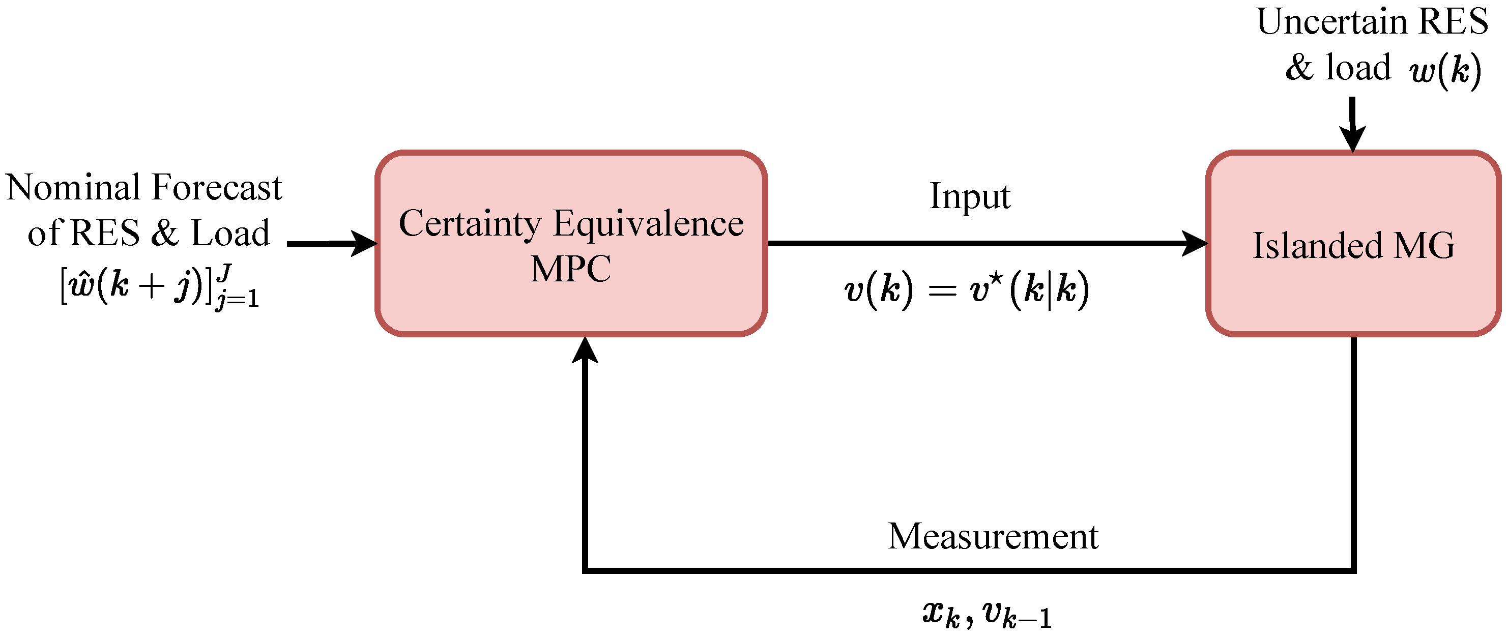
Thus motivated, we extend the works in [22,23] by including the conversion losses in the dynamics of storage units and in the proposed controller to reduce the prediction error in the storage units. We assume the nominal forecast of load and available renewable infeed in the proposed controller, while the uncertain RES and load are considered in the MG model. The closed-loop setup of the proposed certainty equivalence MPC scheme for the operation of an islanded MG is shown in Figure 1.

In brief, the contributions of this work are as follows:

(i)

We derive the model of an islanded MG with uncertain renewable generation and loads with a very high share of RES. This model, motivated by [22], considers a possible limitation of renewable infeed, while limitations on transmission lines are approximately accounted for using DC power flow approximations.

(ii)

We model storage devices as grid-forming units, and, to make the MG model more realistic, we consider the conversion losses of the storage units, the losses of the power electronic devices when converting Alternating Current (AC) to Direct Current (DC) (and vice versa), as well as ohmic losses in the batteries as the quadratic functions in the dynamics of storage units.

(iii)

We take into account power-sharing with the active conventional units. Therefore, the load fluctuations and renewable units influence all units’ power and the storage units’ state of charge. In this way, the model can also work where only RES and storage units are active, and no conventional unit is required.

(iv)

We propose a novel MPC approach for the optimal operation of an islanded MG with a very high share of renewable energy sources. To solve the optimization problem and mitigate the effect of errors in the storage units’ state of charge prediction, we reformulate the conversion loss functions as the mixed-integer linear inequality functions and include them in the proposed scheme.

(v)

We confirm the properties of the proposed operation control scheme via realistic simulations with a high renewable share.

1.3. Paper Organization

This paper is organized as follows. In Section 2, we introduce the model of an islanded MG. Then, we formulate the certainty equivalence MPC problem in Section 3. In Section 4, we introduce the operating costs of the MG. In Section 5, we demonstrate the effectiveness of the resulting MPC in a numerical case study. Lastly, in Section 6, we provide the concluding remarks and possible directions for future research.

1.4. Mathematical Notation

The sets of complex, real, strictly positive, and negative real numbers are denoted by $\mathbb{C}$, $\mathbb{R}$, ${\mathbb{R}}_{<0}$, and ${\mathbb{R}}_{>0}$, respectively. Moreover, the set of non-positive real numbers is ${\mathbb{R}}_{\le 0}$ and the set of positive real numbers including 0 is ${\mathbb{R}}_{\ge 0}$. The set of natural numbers is $\mathbb{N}$, and the set of non-negative integers is ${\mathbb{N}}_0$. Furthermore, the set of Boolean numbers is $\mathbb{B}=\{0,1\}$. For $d\in \mathbb{N}$ and a column vector of $x\in {\mathbb{R}}^d$, let $x^{\prime }$ be its transpose. Given a matrix A, its transpose is denoted by $A^{\prime }$, while its hermitian (complex conjugate) transpose is $A^H$. The matrix A is also non-negative (psd), denoted by $A⪰0$, if A is Hermitian and $z^{H}Az⪰0$ for all $z\in {\mathbb{C}}^n$. Given a complex number z, its real part is denoted by $\mathrm{Re}\left(z\right)$, while the imaginary part of a complex number z is denoted by $\mathrm{Im}\left(z\right)$. Additionally, given a scalar a, its absolute value is defined by $\left|a\right|$. Finally, $I_n$ denotes the n-dimensional identity matrix, and by $1_n$ and $0_n$, respectively, all 1 and all 0 n-dimensional column vectors are represented.

2. Microgrid Model

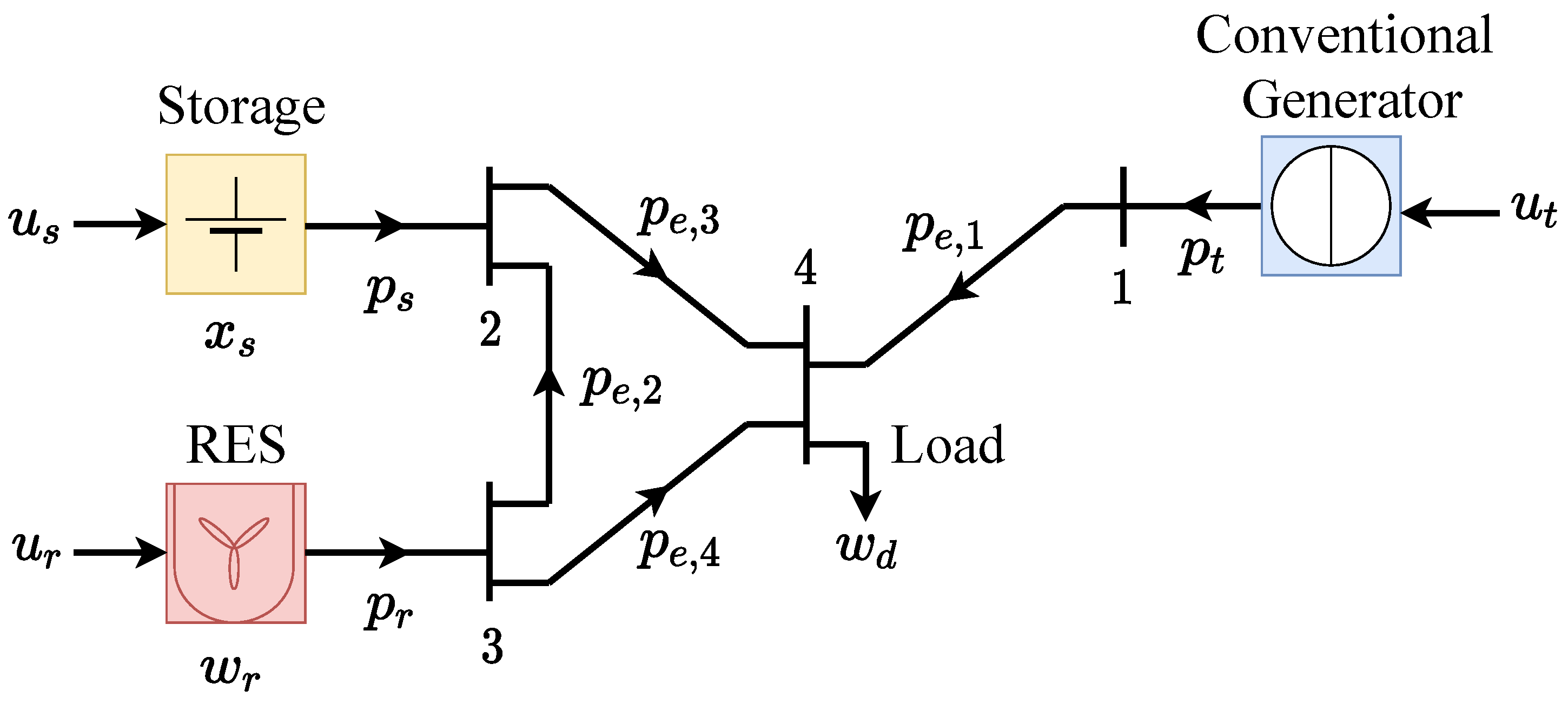
We consider an MG that includes a grouping of conventional generators, renewable energy storage units, and loads connected by transmission lines. Figure 2 depicts a basic MG consisting of all these components. The electrical connection among units and loads due to power lines can be modeled by a di-graph ${\mathcal{G}}_N^e(\mathcal{V},{\mathcal{E}}^e)$, where $\mathcal{V}=\{1,\dots ,N\}$ represents the set of agents and ${\mathcal{E}}^e\subseteq \{\mathcal{V}\times \mathcal{V}\}$ is the set of edges (transmission lines) between two distinct agents. In this manuscript, we consider that the set of agents includes four subsets ${\mathcal{V}}_T$, ${\mathcal{V}}_S$, ${\mathcal{V}}_R$, and ${\mathcal{V}}_L$, wherein these letters denote, respectively, the sets of conventional, energy storage, renewable units, and loads. We also denote by ${\mathcal{Y}}_{ij}=G_{ik}+ı·B_{ij}\in \mathbb{C}$ the admittance line between the i-th agent and j-th agent, wherein $G_{ij}$ and $B_{ij}$ show the line conductance and susceptance between the i-th agent and j-th agent. If no connection between the i-th agent and j-th agent exists, $G_{ij}=B_{ij}=0$.

With the variables summarized in

Table 1. Model-specific variables.

Symbol	Explanation	Unit	Size
x	Energy of storage units (state)	$\mathrm{pu}\mathrm{h}$	S
$u_{\mathrm{t}}$	Setpoint inputs of conventional units	$\mathrm{pu}$	T
$u_{\mathrm{s}}$	Setpoint inputs of storage units	$\mathrm{pu}$	S
$u_{\mathrm{r}}$	Setpoint inputs of renewable units	$\mathrm{pu}$	R
u	Setpoint inputs of all units	$\mathrm{pu}$	U
${\delta }_{\mathrm{t}}$	Boolean inputs of conventional units	-	T
v	Vector of all control inputs	-	Q
$w_{\mathrm{r}}$	Uncertain available renewable power	$\mathrm{pu}$	R
$w_{\mathrm{d}}$	Uncertain load	$\mathrm{pu}$	D
w	Vector of all uncertain inputs	$\mathrm{pu}$	W
$p_{\mathrm{t}}$	Active power of conventional units	$\mathrm{pu}$	T
$p_{\mathrm{s}}$	Active power of storage units	$\mathrm{pu}$	S
$p_{\mathrm{r}}$	Active power of renewable units	$\mathrm{pu}$	R
p	Active power of all units	$\mathrm{pu}$	U
$p_{\mathrm{e}}$	Power over transmission lines	$\mathrm{pu}$	E
${\delta }_{\mathrm{r}}$	Boolean auxiliary variables	-	R
$\rho$	Real-valued auxiliary variable	-	1
$\overline{q}$	Vector of all auxiliary variables	-	Q

, the behavior of the MG is modeled by:

$$\begin{array}{}\mathrm{(1a)}& \hfill x(k+1)& =x\left(k\right)-T_s·\left\{B·\overline{q}\left(k\right)+\mathbb{F}\left(k\right)\right\},\hfill \mathrm{(1b)}& \hfill h_1& \ge H_1·x(k+1),\hfill \mathrm{(1c)}& \hfill h_2& \ge H_2·{\left[\begin{array}{ccc}v{\left(k\right)}^{\prime }& \overline{q}{\left(k\right)}^{\prime }& w{\left(k\right)}^{\prime }\end{array}\right]}^{\prime },\hfill \mathrm{(1d)}& \hfill g& =G·{\left[\begin{array}{ccc}v{\left(k\right)}^{\prime }& \overline{q}{\left(k\right)}^{\prime }& w{\left(k\right)}^{\prime }\end{array}\right]}^{\prime },\hfill \end{array}$$

where $k\in {\mathbb{N}}_0$ is the time index, $x\left(k\right)\in {\mathbb{R}}_{\ge 0}^S$ with $S\in \mathbb{N}$ is the state vector with initial value $x_0\in {\mathbb{R}}_{\ge 0}^S$. In fact, this vector is inclusive of entries $x_i\left(k\right)$ that represent the stored energy of unit $i\in {\mathbb{N}}_{[1,S]}$. $\overline{q}\left(k\right)\in {\mathbb{R}}^Q$ is referred to as a vector of $Q\in \mathbb{N}$ auxiliary variables. $\mathbb{F}\left(k\right)$ is a vector of $S\in \mathbb{N}$ in which each of its elements represent the function of the conversion losses. $v\left(k\right)={\left[u{\left(k\right)}^{\prime }{\delta }_t{\left(k\right)}^{\prime }\right]}^{\prime }$ is also the vector of control inputs, wherein $u\left(k\right)\in {\mathbb{R}}^U$ is denoted as the vector of the real-valued control inputs of all $U\in \mathbb{N}$ units and ${\delta }_t\left(k\right)\in {\{0,1\}}^T$ is defined to be the vector of $T\in \mathbb{N}$ Boolean inputs. The uncertain external input is also collected in the vector $w\left(k\right)={\left[w_r{\left(k\right)}^{\prime }{w}_t{\left(k\right)}^{\prime }\right]}^{\prime }$, where $w_r\left(k\right)$ is the maximum infeed under weather conditions of all renewable units and $w_t\left(k\right)$ includes all loads, $W\in \mathbb{N}$. Let $B\in {\mathbb{R}}^{S\times Q}$ in (1a) and $H_1$, $h_1$ in (1b) be appropriate dimensions. Furthermore, we consider in (1c), $H_2$ and $h_2$, respectively, as a matrix and a vector of appropriate dimensions that reflect inequality constraints. Likewise, in (1d), G is a matrix and g a vector of appropriate dimensions that reflect equality constraints. In more detail, the real-valued control inputs are the power setpoints of the units $u\left(k\right)={\left[u_t{\left(k\right)}^{\prime }{u}_s{\left(k\right)}^{\prime }{u}_r{\left(k\right)}^{\prime }\right]}^{\prime }$, where $u_t{\left(k\right)}^{\prime }\in {\mathbb{R}}_{\ge 0}^T$ is related to the conventional units, $u_s{\left(k\right)}^{\prime }\in {\mathbb{R}}^S$ to the storage units, and $u_r\left(k\right)\in {\mathbb{R}}_{\ge 0}^R$ to the renewable units, such as wind turbines and PV power plants. Regarding the storage and conventional generators, $u_s\left(k\right)$ and $u_t\left(k\right)$ represent desired power values. For RES, $u_r\left(k\right)$ represents an upper limit on the weather-dependent power infeed. Hence, $u_r\left(k\right)$ is their maximum admissible value.

Furthermore, for each conventional generator, a Boolean control input ${\delta }_{t,i}\left(k\right)\in \{0,1\}$ is considered. This input shows whether generator $i\in {\mathbb{N}}_{[1,T]}$ is active (${\delta }_{t,i}\left(k\right)=1$) or inactive (${\delta }_{t,i}\left(k\right)=0$). The Boolean variables of all conventional generators are gathered in the vector ${\delta }_t$.

In what follows, we will derive a control-oriented MG model of the form (1). We start by posing some assumptions.

Assumption 1

(Lower control layers). The lower control layers, i.e., primary and secondary control, are considered to compensate for the frequency and voltage deviations by providing setpoints to the units, as well as establishing the power-sharing (see, e.g., [6,26,27]) among the grid-forming units. Notice that the MG can run autonomously in these layers for several minutes.

Assumption 2

(Conventional units). In terms of time, conventional units have shorter start-up and shutdown times than the sampling time of (MPC), meaning that switching actions are supposed to be instantaneous. Furthermore, changes in power are instantaneous, i.e., no climb rates need to be considered.

Assumption 3

(RES units and loads). It is assumed that the uncertain input follows the nominal forecast of load and available renewable infeed.

Assumption 4

(Transmission lines). It is assumed that the resistance of the electrical coupling among units and loads of MG as well as reactive power flow is negligible. Since the voltage amplitudes in the network are constant, and the phase angle differences small, the DC power flow approximations [28] can be employed.

3. Certainty Equivalence Model Predictive Control

3.1. Plant Model Interface

The power setpoints of the units $u\left(k\right)={\left[u_t{\left(k\right)}^{\prime }{u}_s{\left(k\right)}^{\prime }{u}_r{\left(k\right)}^{\prime }\right]}^{\prime }\in {\mathbb{R}}^U$, called the real-valued manipulated variables containing $u_t{\left(k\right)}^{\prime }\in {\mathbb{R}}_{\ge 0}^T$ as setpoints of the T conventional units, $u_s{\left(k\right)}^{\prime }\in {\mathbb{R}}^S$ the setpoints of the S storage units and $u_r\left(k\right)\in {\mathbb{R}}_{\ge 0}^R$ the setpoints of the R (RES). To show that conventional units are enabled or disabled, we consider a Boolean input for each conventional unit and we collect all Boolean inputs in a vector ${\delta }_t\left(k\right)\in {\{0,1\}}^T$. Moreover, the stored energies of the storage units are gathered in the state vector $x\left(k\right)\in {\mathbb{R}}_{\ge 0}^S$. The uncertain external input of the model is expressed by $w\left(k\right)={\left[w_r{\left(k\right)}^{\prime }{w}_d{\left(k\right)}^{\prime }\right]}^{\prime }$, where $w_r\left(k\right)\in {\mathbb{R}}_{\ge 0}^R$ shows the maximum available power of the renewable units under given weather conditions and $w_d\left(k\right)\in {\mathbb{R}}_{\ge 0}^D$ the load.

3.2. Power of Units

We consider $p\left(k\right)={\left[p_t{\left(k\right)}^{\prime }{p}_s{\left(k\right)}^{\prime }{p}_r{\left(k\right)}^{\prime }\right]}^{\prime }$ as the vector of power values, which consists of the power of conventional units, $p_t\left(k\right)\in {\mathbb{R}}_{\ge 0}^T$, storage units, $p_s\in {\mathbb{R}}^S$, and RES, $p_r\left(k\right)\in {\mathbb{R}}_{\ge 0}^R$. It is worth noting that, in islanded mode, since production, consumption, and storage power must be balanced in the presence of uncertain load and renewable infeed, the power of the units $p\left(k\right)\in {\mathbb{R}}^U$ is not necessarily equal to the setpoints $u\left(k\right)$.

3.2.1. Active Power at RES Units

Let the active power of renewable units, $p_{\mathrm{r}}\left(k\right)$, as well as the corresponding setpoints, $u_{\mathrm{r}}\left(k\right)$, be bounded by:

$$\begin{array}{cccc}\hfill p_{\mathrm{r}}^{min}& \le p_r\left(k\right)\hfill & & \le p_{\mathrm{r}}^{max},\hfill \end{array}$$

(2a)

$$\begin{array}{cccc}\hfill p_{\mathrm{r}}^{min}& \le u_r\left(k\right)\hfill & & \le p_{\mathrm{r}}^{max}.\hfill \end{array}$$

(2b)

Furthermore, we consider that the power infeed $p_{\mathrm{r},i}\left(k\right)\in {\mathbb{R}}_{\ge 0}$ of any renewable unit $i\in {\mathcal{N}}_{[1,R]}$ can be constrained by the power setpoint $u_{\mathrm{r},i}\left(k\right)\in {\mathbb{R}}_{\ge 0}$. Notice that the power tracks the setpoint when the maximum possible infeed under current weather conditions $w_{\mathrm{r},i}\left(k\right)\in {\mathbb{R}}_{\ge 0}$ is greater than or equal to $u_{\mathrm{r},i}\left(k\right)$. This can be characterized by using the element-wise min operator as follows:

$$p_r\left(k\right)=min(u_r\left(k\right),w_r\left(k\right)).$$

(3)

To solve the optimization problem, the authors in [22] reformulated (3) to a set of linear inequalities including integer variables as follows:

$$\begin{array}{cc}\hfill p_{\mathrm{r}}\left(k\right)& \le u_{\mathrm{r}}\left(k\right),\hfill \end{array}$$

(4a)

$$\begin{array}{cc}\hfill p_{\mathrm{r}}\left(k\right)& \ge u_{\mathrm{r}}\left(k\right)+(diag\left(w_{\mathrm{r}}\left(k\right)\right)-{\mathrm{M}}_{\mathrm{r}}{I}_R){\delta }_{\mathrm{r}}\left(k\right),\hfill \end{array}$$

(4b)

$$\begin{array}{cc}\hfill p_{\mathrm{r}}\left(k\right)& \le w_{\mathrm{r}}\left(k\right),\hfill \end{array}$$

(4c)

$$\begin{array}{cc}\hfill p_{\mathrm{r}}\left(k\right)& \ge w_{\mathrm{r}}\left(k\right)-(diag\left(w_{\mathrm{r}}\left(k\right)\right)-{\mathrm{m}}_{\mathrm{r}}{I}_R)(1_R-{\delta }_{\mathrm{r}}\left(k\right)).\hfill \end{array}$$

(4d)

where ${\delta }_{\mathrm{r}}\left(k\right)\in {\{0,1\}}^R$ represents the free variable and ${\mathrm{m}}_{\mathrm{r}}\in \mathbb{R}$, ${\mathrm{m}}_{\mathrm{r}}<min\left(p_{\mathrm{r}}^{min}\right)$ and ${\mathrm{M}}_{\mathrm{r}}\in {\mathbb{R}}_{\ge 0}$, ${\mathrm{M}}_{\mathrm{r}}>max\left(p_{\mathrm{r}}^{max}\right)$ are the constant coefficients, which are computed offline.

3.2.2. Active Power at Conventional Units

We consider whether the conventional unit $i\in {\mathcal{N}}_{[1,T]}$ is enabled, i.e., if ${\delta }_{\mathrm{t},i}\left(k\right)=1$, then its active power is bounded by $p_{\mathrm{t},i}^{min}\in {\mathbb{R}}_{\ge 0}$ and $p_{\mathrm{t},i}^{max}\in {\mathbb{R}}_{\ge 0}$. If the unit is disabled, i.e., ${\delta }_{\mathrm{t},i}\left(k\right)=0$, then, naturally, $p_{\mathrm{t},i}\left(k\right)=0$. The active power of conventional units with $p_{\mathrm{t}}^{min}\in {\mathbb{R}}_{\ge 0}^T$, $p_{\mathrm{t}}^{max}\in {\mathbb{R}}_{\ge 0}^T$ can be written in vector form as [22]:

$$diag\left(p_{\mathrm{t}}^{min}\right){\delta }_{\mathrm{t}}\left(k\right)\le p_{\mathrm{t}}\left(k\right)\le diag\left(p_{\mathrm{t}}^{max}\right){\delta }_{\mathrm{t}}\left(k\right),$$

(5a)

The same holds for the active power setpoints, i.e.,

$$diag\left(p_{\mathrm{t}}^{min}\right){\delta }_{\mathrm{t}}\left(k\right)\le u_{\mathrm{t}}\left(k\right)\le diag\left(p_{\mathrm{t}}^{max}\right){\delta }_{\mathrm{t}}\left(k\right).$$

(5b)

3.2.3. Active Power at Storage Units

Since we assume that all storage units are always enabled, all their active power setpoints and active power values are bounded as:

$$\begin{array}{ccc}\hfill p_{\mathrm{s}}^{min}& \le p_{\mathrm{s}}\left(k\right)\hfill & \le p_{\mathrm{s}}^{max},\hfill \end{array}$$

(6a)

$$\begin{array}{ccc}\hfill p_{\mathrm{s}}^{min}& \le u_{\mathrm{s}}\left(k\right)\hfill & \le p_{\mathrm{s}}^{max}.\hfill \end{array}$$

(6b)

where $p_{\mathrm{s}}^{min}\in {\mathbb{R}}_{\le 0}^S$ and $p_{\mathrm{s}}^{max}\in {\mathbb{R}}_{\ge 0}^S$ represent the known lower and upper power limits.

3.3. Power Sharing of Grid-Forming Units

Note that the power of all units does not necessarily equal the power setpoints that are assigned to the system due to variations in load and renewable infeed. Therefore, we assume that the secondary and primary control layers control all units to share the changes in load and renewable infeed in a desired proportional manner. The aforementioned so-called proportional power-sharing (see, e.g., [27,29]) depends on the design parameter ${\chi }_i\in {\mathbb{R}}_{>0}$ for all grid-forming units. A practical option for ${\chi }_i$ is, e.g., proportional to the nominal power of the corresponding units.

Power sharing can be described by (7), where two units $i\in {\mathcal{N}}_{[1,T+S]}$ and $j\in {\mathcal{N}}_{[1,T+S]}$, $i\ne j$ share their active power proportionally according to ${\chi }_i\in {\mathbb{R}}_{>0}$ and ${\chi }_j\in {\mathbb{R}}_{>0}$, if the next relation holds:

$$\frac{p_i\left(k\right)-u_i\left(k\right)}{{\chi }_i}=\frac{p_j\left(k\right)-u_j\left(k\right)}{{\chi }_j}$$

(7)

By using a new auxiliary free variable $\rho \left(k\right)\in \mathbb{R}$ and considering that only enabled units, namely units i with ${\delta }_{\mathrm{t},i}\left(k\right)=1$, can participate in power-sharing, (7) can be recast for all grid-forming units with $K_{\mathrm{t}}=diag\left({[\frac{1}{{\chi }_1}\dots \frac{1}{{\chi }_T}]}^{\prime }\right)$ and $K_{\mathrm{s}}=diag\left({[\frac{1}{{\chi }_{(T+1)}}\dots \frac{1}{{\chi }_{(T+S)}}]}^{\prime }\right)$ as [22]:

$$\begin{array}{cc}\hfill K_{\mathrm{t}}(p_{\mathrm{t}}\left(k\right)-u_{\mathrm{t}}\left(k\right))& =\rho \left(k\right){\delta }_{\mathrm{t}}\left(k\right)\mathrm{and}\hfill \end{array}$$

(8a)

$$\begin{array}{cc}\hfill K_{\mathrm{s}}(p_{\mathrm{s}}\left(k\right)-u_{\mathrm{s}}\left(k\right))& =\rho \left(k\right)1_S.\hfill \end{array}$$

(8b)

For the formulation of the optimisation problem, ref. [22] transforms (8a) into the following set of linear inequalities with integer variables:

$$\begin{array}{cc}\hfill K_{\mathrm{t}}(p_{\mathrm{t}}\left(k\right)-u_{\mathrm{t}}\left(k\right))& \le {\mathrm{M}}_{\mathrm{t}}{\delta }_{\mathrm{t}}\left(k\right),\hfill \end{array}$$

(9a)

$$\begin{array}{cc}\hfill K_{\mathrm{t}}(p_{\mathrm{t}}\left(k\right)-u_{\mathrm{t}}\left(k\right))& \ge {\mathrm{m}}_{\mathrm{t}}{\delta }_{\mathrm{t}}\left(k\right),\hfill \end{array}$$

(9b)

$$\begin{array}{cc}\hfill K_{\mathrm{t}}(p_{\mathrm{t}}\left(k\right)-u_{\mathrm{t}}\left(k\right))& \le 1_T\rho \left(k\right)-{\mathrm{m}}_{\mathrm{t}}(1_T-{\delta }_{\mathrm{t}}\left(k\right)),\hfill \end{array}$$

(9c)

$$\begin{array}{cc}\hfill K_{\mathrm{t}}(p_{\mathrm{t}}\left(k\right)-u_{\mathrm{t}}\left(k\right))& \ge 1_T\rho \left(k\right)-{\mathrm{M}}_{\mathrm{t}}(1_T-{\delta }_{\mathrm{t}}\left(k\right)).\hfill \end{array}$$

(9d)

where ${\mathrm{M}}_{\mathrm{t}}\in \mathbb{R}$ can be calculated offline and its value should be greater than the largest possible value of $\rho \left(k\right)$. Hence, with the largest possible value for the storage units, ${\rho }_{\mathrm{s}}^{max}=max\left(K_{\mathrm{s}}(p_{\mathrm{s}}^{max}-p_{\mathrm{s}}^{min})\right)$, and for the conventional units, ${\rho }_{\mathrm{t}}^{max}=max\left(K_{\mathrm{t}}(p_{\mathrm{t}}^{max}-p_{\mathrm{t}}^{min})\right)$, ${\mathrm{M}}_{\mathrm{t}}$ has to be chosen such that $max\left({\rho }_{\mathrm{s}}^{max},{\rho }_{\mathrm{t}}^{max}\right)<{\mathrm{M}}_{\mathrm{t}}$. Moreover, ${\mathrm{m}}_{\mathrm{t}}=-{\mathrm{M}}_{\mathrm{t}}$.

3.4. Dynamics of Storage Units

The dynamics of all storage units can be formulated as:

$$x(k+1)=x\left(k\right)-{\mathrm{T}}_{\mathrm{s}}{p}_{\mathrm{s}}\left(k\right)-{\mathrm{T}}_{\mathrm{s}}\mathbb{F}\left(p_{\mathrm{s}}\left(k\right)\right),$$

(10)

where ${\mathrm{T}}_{\mathrm{s}}\in {\mathbb{R}}_{>0}$ is the sampling time and $x\left(k\right)$ represents the stored energy with initial state $x\left(0\right)=x_0$. The constraint of the stored energy is given by:

$$x^{min}\le x(k+1)\le x^{max},$$

(11)

with $x^{min}=0_S$ and $x^{max}\in {\mathbb{R}}_{\ge 0}^S$. In particular, $\mathbb{F}\left(p_{\mathrm{s}}\left(k\right)\right)={[f_1\left(p_{\mathrm{s},1}\left(k\right)\right),\dots ,f_S\left(p_{\mathrm{s},\mathrm{S}}\left(k\right)\right)]}^{\prime }$ is a vector of $S\in \mathbb{N}$, where each of its elements represents the conversion loss terms, including the conversion losses of the storage units, the losses of the power electronic devices when converting AC to DC (and vice versa), as well as ohmic losses in the batteries, considered to be a convex quadratic function as follows:

$$f_i\left(p_{\mathrm{s},\mathrm{i}}\left(k\right)\right)=a{p}_{\mathrm{s},\mathrm{i}}{\left(k\right)}^2+b{p}_{\mathrm{s},\mathrm{i}}\left(k\right)+c,a,b,c\in \mathbb{R}$$

(12)

where $p_{\mathrm{s},\mathrm{i}}\left(k\right)$ is assumed to be limited as:

$$p_{\mathrm{s},\mathrm{i}}\left(k\right)\in {\mathcal{D}}_i=\left\{p_{\mathrm{s},\mathrm{i}}\left(k\right)|p_{s,i}^{min}\le p_{\mathrm{s},\mathrm{i}}\left(k\right)\le p_{s,i}^{max}\right\}$$

(13)

Note that the polynomial function, $f_i\left(p_{\mathrm{s},\mathrm{i}}\left(k\right)\right)$, is an example and it could be replaced by some other complex functions for different storage technology. Moreover, the coefficients are found offline by looking at the storage units and analyzing measurements.

To solve the optimization problem, it is useful to reformulate the function $f\left(p_{\mathrm{s},\mathrm{i}}\left(k\right)\right)$ as piecewise affine functions (see, e.g., [30]), i.e.,

$$f_i\left(p_{s,i}\left(k\right)\right)=\left\{\begin{array}{cc}{A}_{1,i}{p}_{s,i}\left(k\right)+B_{1,i},\hfill & p_{s,i}\left(k\right)\in {\mathcal{D}}_{1,i},\hfill \\ A_{2,i}ps,i\left(k\right)+B_{2,i},\hfill & p_{s,i}\left(k\right)\in {\mathcal{D}}_{2,i},\hfill \\ ⋮\hfill \\ A_{r,i}{p}_{s,i}\left(k\right)+B_{r,i},\hfill & p_{s,i}\left(k\right)\in {\mathcal{D}}_{r,i}.\hfill \end{array}\right.$$

(14)

in which $A_{y,i}$, $B_{y,i}\in \mathbb{R}$ and the following holds:

$$\bigcup _{1\le y\le r}{\mathcal{D}}_{y,i}={\mathcal{D}}_i$$

(15a)

$$\bigcap _{1\le y\le r}{\mathcal{D}}_{y,i}=0$$

(15b)

and, on the borders of sequential ${\mathcal{D}}_y$, the linear segments are connected, which means that $f_i\left(p_{s,i}\left(k\right)\right)$ is continuous.

The condition $p_{s,i}\left(k\right)$ at each partition ${\mathcal{D}}_{y,i}$ can be associated with a binary variable ${\delta }_{y,i}\left(k\right)\in \{0,1\}$, $\forall y=1,2,\dots ,r$, satisfying the exclusive-or condition:

$$\underset{y=1}{\overset{r}{⨁}}[{\delta }_{y,i}\left(k\right)=1].$$

(16)

such that:

$$[{\delta }_{y,i}\left(k\right)=1]⟷p_{s,i}\left(k\right)\in {\mathcal{D}}_{y,i}$$

(17)

From (16), there exists some ${\delta }_{y,i}\left(k\right)=1$, which implies $p_{s,i}\left(k\right)\in {\mathcal{D}}_{y,i}$, a contradiction by (15b). Therefore, (15)–(17) are equivalent to:

$${\mathbb{J}}_{y,i}^T{p}_{s,i}\left(k\right)-{\mathbb{H}}_{y,i}^T\le {\mathbb{M}}_i^{★}[1-{\delta }_{y,i}\left(k\right)]$$

(18a)

$$\sum _{y=1}^r{\delta }_{y,i}\left(k\right)=1$$

(18b)

with ${\mathbb{J}}_{y,i}=\left[\begin{array}{cc}1& -1\end{array}\right]$ for $y=\{1,\dots ,r\}$ and $i=\{1,\dots ,S\}$, and ${\mathbb{H}}_{y,i}$ represents a vector of 2, where the first row of ${\mathbb{H}}_{y,i}$ is equal to the lower bound of the $D_{y,i}$ with a minus sign, while its second row is the upper bound. ${\mathbb{M}}_i^{★}$ in (18a) can be computed as:

$${\mathbb{M}}_i^{★}\cong \underset{p_{s,i}\left(k\right)\in {\mathcal{D}}_i}{max}{\mathbb{J}}_{y,i}^T{p}_{s,i}\left(k\right)-{\mathbb{H}}_{y,i}^T$$

(19)

By using this binary variable, we can recast (14) as follows (see, e.g., [30]):

$$f_i\left(p_{\mathrm{s},\mathrm{i}}\left(k\right)\right)=\left\{\begin{array}{cc}{A}_{1,i}{p}_{\mathrm{s},\mathrm{i}}\left(k\right)+B_{1,i},\hfill & \mathrm{if}{\delta }_{1,i}\left(k\right)=1,\hfill \\ A_{2,i}{p}_{\mathrm{s},\mathrm{i}}\left(k\right)+B_{2,i},\hfill & \mathrm{if}{\delta }_{2,i}\left(k\right)=1,\hfill \\ ⋮\hfill \\ A_{r,i}{p}_{\mathrm{s},\mathrm{i}}\left(k\right)+B_{r,i},\hfill & \mathrm{if}{\delta }_{r,i}\left(k\right)=1.\hfill \end{array}\right.$$

(20)

Therefore, (20) can be rewritten as:

$$f_i\left(p_{\mathrm{s},\mathrm{i}}\left(k\right)\right)=\sum _{y=1}^r[A_{y,i}{p}_{\mathrm{s},\mathrm{i}}\left(k\right)+B_{y,i}]{\delta }_{y,i}\left(k\right).$$

(21)

Unfortunately, (21) is nonlinear since it involves products between logical variables and inputs. Therefore, we transform it into equivalent mixed-integer linear inequalities. This can be done using a similar strategy as proposed in [30]. To this aim, we set:

$$f_i\left(p_{\mathrm{s},\mathrm{i}}\left(k\right)\right)=\sum _{y=1}^r{z}_{y,i}\left(k\right)$$

(22a)

$$z_{y,i}\left(k\right)\cong [A_{y,i}{p}_{s,i}\left(k\right)+B_{y,i}]{\delta }_{y,i}\left(k\right).$$

(22b)

Then, (22b) is equivalent to:

$$\begin{array}{cc}\hfill z_{y,i}\left(k\right)& \le {\tilde{M}}_i{\delta }_{y,i}\left(k\right),\hfill \\ \hfill z_{y,i}\left(k\right)& \ge {\tilde{m}}_i{\delta }_{y,i}\left(k\right),\hfill \end{array}$$

$$\begin{array}{cc}\hfill z_{y,i}\left(k\right)& \le A_{y,i}{p}_{s,i}\left(k\right)+B_{y,i}-{\tilde{m}}_i(1-{\delta }_{y,i}\left(k\right)),\hfill \end{array}$$

(23)

$$\begin{array}{cc}\hfill z_{y,i}\left(k\right)& \ge A_{y,i}{p}_{s,i}\left(k\right)+B_{y,i}-{\tilde{M}}_i(1-{\delta }_{y,i}\left(k\right)).\hfill \end{array}$$

(24)

being

$${\tilde{M}}_i\cong \underset{y=1,\dots ,r}{max}\left\{\underset{p_{s,i}\left(k\right)\in {\mathcal{D}}_i}{max}{A}_{i,y}{p}_{s,i}\left(k\right)+B_{i,y}\right\}.$$

(25a)

$${\tilde{m}}_i\cong \underset{y=1,\dots ,r}{min}\left\{\underset{p_{s,i}\left(k\right)\in {\mathcal{D}}_i}{max}{A}_{i,y}{p}_{s,i}\left(k\right)+B_{i,y}\right\}.$$

(25b)

Remark 1.

Notice that, in [22], the dynamics of all storage units are considered without piecewise affine losses terms, namely,

$$x(k+1)=x\left(k\right)-{\mathrm{T}}_{\mathrm{s}}{p}_{\mathrm{s}}\left(k\right),$$

(26)

with

$$x^{min}\le x(k+1)\le x^{max},$$

(27)

3.5. Transmission Network

Following [24], the DC power flow approximations can be employed to extract the power of transmission lines, $p_e\left(k\right)={\left[\begin{array}{ccc}{p}_{e,1}\left(k\right)& \dots & p_{e,E}\left(k\right)\end{array}\right]}^{\prime }$. Hence, the power on lines can be formulated from the power of units and load using the following linear equation:

$$\begin{array}{cc}\hfill p_e\left(k\right)=& F·{\left[p{\left(k\right)}^{\prime }{w}_d{\left(k\right)}^{\prime }\right]}^{\prime },\hfill \end{array}$$

(28a)

where $F\in {\mathbb{R}}^{E\times (U+D)}$ represents a matrix that links the power flowing over the lines with the power produced or consumed by the units and loads. More details about the derivation of F are provided in [31]. It is assumed that $p_e\left(k\right)$ is bounded by:

$$p_e^{min}\le p_e\left(k\right)\le p_e^{max}$$

(28b)

with $p_e^{min}\in {\mathbb{R}}_{\le 0}^E$ and $p_e^{max}\in {\mathbb{R}}_{\ge 0}^E$. This assumption is reasonable due to the physical limitation in the transmission capability of the lines. Moreover, the produced power must be equal to the consumed power at all times [24], e.g.,

$$1_T^{\prime }{p}_t\left(k\right)+1_S^{\prime }{p}_s\left(k\right)+1_R^{\prime }{p}_r\left(k\right)=1_D^{\prime }{w}_d\left(k\right).$$

(28c)

3.6. Overall Model

In accordance with the equations considered for the different parts of an islanded MG, the overall model can be formulated as follows. The constraints on power and setpoint originate from (2), (5) and (6), namely,

$$\begin{array}{cc}\hfill \left[\begin{array}{c}diag\left(p_{\mathrm{t}}^{max}\right){\delta }_{\mathrm{t}}\left(k\right)\\ p_{\mathrm{s}}^{max}\\ p_{\mathrm{r}}^{max}\end{array}\right]& \le u\left(k\right)\le \left[\begin{array}{c}diag\left(p_{\mathrm{t}}^{min}\right){\delta }_{\mathrm{t}}\left(k\right)\\ p_{\mathrm{s}}^{min}\\ p_{\mathrm{r}}^{min}\end{array}\right]\hfill \end{array}$$

(29a)

and

$$\begin{array}{cc}\hfill \left[\begin{array}{c}diag\left(p_{\mathrm{t}}^{max}\right){\delta }_{\mathrm{t}}\left(k\right)\\ p_{\mathrm{s}}^{max}\\ p_{\mathrm{r}}^{max}\end{array}\right]& \le p\left(k\right)\le \left[\begin{array}{c}diag\left(p_{\mathrm{t}}^{min}\right){\delta }_{\mathrm{t}}\left(k\right)\\ p_{\mathrm{s}}^{min}\\ p_{\mathrm{r}}^{min}\end{array}\right]\hfill \end{array}$$

(29b)

By referring to (10), the dynamics of the storage unit are described by:

$$x(k+1)=x\left(k\right)-{\mathrm{T}}_{\mathrm{s}}{p}_{\mathrm{s}}\left(k\right)-{\mathrm{T}}_{\mathrm{s}}{[f_1\left(p_{\mathrm{s},1}\left(k\right)\right),\dots ,f_S\left(p_{\mathrm{s},\mathrm{S}}\left(k\right)\right)]}^{\prime },$$

(29c)

with constraint functions

$$x^{min}\le x(k+1)\le x^{max},$$

(29d)

$$f_i\left(p_{\mathrm{s},\mathrm{i}}\left(k\right)\right)=\sum _{y=1}^r{z}_{y,i}\left(k\right)$$

(29e)

$$\begin{array}{cc}\hfill z_{y,i}\left(k\right)& \le {\tilde{M}}_i{\delta }_{y,i}\left(k\right),\hfill \\ \hfill z_{y,i}\left(k\right)& \ge {\tilde{m}}_i{\delta }_{y,i}\left(k\right),\hfill \\ \hfill z_{y,i}\left(k\right)& \le A_{y,i}{p}_{s,i}\left(k\right)+B_{y,i}-{\tilde{m}}_i(1-{\delta }_{y,i}\left(k\right)),\hfill \\ \hfill z_{y,i}\left(k\right)& \ge A_{y,i}{p}_{s,i}\left(k\right)+B_{y,i}-{\tilde{M}}_i(1-{\delta }_{y,i}\left(k\right)).\hfill \end{array}$$

(29f)

The renewable infeed, which is a function of the setpoint and the available power under weather conditions, is given by (4) as:

$$\begin{array}{cc}\hfill p_{\mathrm{r}}\left(k\right)& \le u_{\mathrm{r}}\left(k\right),\hfill \end{array}$$

(29g)

$$\begin{array}{cc}\hfill p_{\mathrm{r}}\left(k\right)& \ge u_{\mathrm{r}}\left(k\right)+(diag\left(w_{\mathrm{r}}\left(k\right)\right)-{\mathrm{M}}_{\mathrm{r}}{I}_R){\delta }_{\mathrm{r}}\left(k\right),\hfill \end{array}$$

(29h)

$$\begin{array}{cc}\hfill p_{\mathrm{r}}\left(k\right)& \le w_{\mathrm{r}}\left(k\right),\hfill \end{array}$$

(29i)

$$\begin{array}{cc}\hfill p_{\mathrm{r}}\left(k\right)& \ge w_{\mathrm{r}}\left(k\right)-(diag\left(w_{\mathrm{r}}\left(k\right)\right)-{\mathrm{m}}_{\mathrm{r}}{I}_R)(1_R-{\delta }_{\mathrm{r}}\left(k\right)).\hfill \end{array}$$

(29j)

Power-sharing of the grid-forming units is described by (8), which, using (9), can be recast into:

$$\begin{array}{cc}\hfill K_{\mathrm{t}}(p_{\mathrm{t}}\left(k\right)-u_{\mathrm{t}}\left(k\right))& \le {\mathrm{M}}_{\mathrm{t}}{\delta }_{\mathrm{t}}\left(k\right),\hfill \end{array}$$

(29k)

$$\begin{array}{cc}\hfill K_{\mathrm{t}}(p_{\mathrm{t}}\left(k\right)-u_{\mathrm{t}}\left(k\right))& \ge {\mathrm{m}}_{\mathrm{t}}{\delta }_{\mathrm{t}}\left(k\right),\hfill \end{array}$$

(29l)

$$\begin{array}{cc}\hfill K_{\mathrm{t}}(p_{\mathrm{t}}\left(k\right)-u_{\mathrm{t}}\left(k\right))& \le 1_T\rho \left(k\right)-{\mathrm{m}}_{\mathrm{t}}(1_T-{\delta }_{\mathrm{t}}\left(k\right)),\hfill \end{array}$$

(29m)

$$\begin{array}{cc}\hfill K_{\mathrm{t}}(p_{\mathrm{t}}\left(k\right)-u_{\mathrm{t}}\left(k\right))& \ge 1_T\rho \left(k\right)-{\mathrm{M}}_{\mathrm{t}}(1_T-{\delta }_{\mathrm{t}}\left(k\right)).\hfill \end{array}$$

(29n)

Lastly, the power limit of the transmission lines is introduced by (28), i.e.,

$$p_e^{min}\le F·{\left[p_t{\left(k\right)}^{\prime }{}^{\prime }{p}_s{\left(k\right)}^{\prime }{}^{\prime }{p}_r{\left(k\right)}^{\prime }{w}_d{\left(k\right)}^{\prime }\right]}^{\prime }\le p_e^{max}$$

(29o)

$$1_T^{\prime }{p}_t\left(k\right)+1_S^{\prime }{p}_s\left(k\right)+1_R^{\prime }{p}_r\left(k\right)=1_D^{\prime }{w}_d\left(k\right).$$

(29p)

Now, let us compute a compact form of (29). From (29c) and by denoting $\overline{q}{\left(k\right)=[p\left(k\right)}^{\prime }{\delta }_{\mathrm{r}}{\left(k\right)}^{\prime }$${\rho \left(k\right)]}^{\prime }$ and $B=\left[0_{S\times T}{I}_S{0}_{S\times 2R+1}\right]$, we can obtain Equation (1a), namely,

$$\begin{array}{cc}\hfill x(k+1)& =x\left(k\right)-T_s·\left\{B·\overline{q}\left(k\right)+\mathbb{F}\left(k\right)\right\},\hfill \end{array}$$

(30a)

By following (29d), we have

$$\begin{array}{cc}\hfill H_1·x(k+1)& \le h_1,\hfill \end{array}$$

(30b)

with $H_1=diag\left({[1_S^{\prime }-1_S^{\prime }]}^{\prime }\right)$ and $h_1=[{\left(x^{max}\right)}^{\prime }$${(-x^{min})}^{\prime }{]}^{\prime }$.

Finally, according to (29a) and (29b) and (29n)–(29p), the next equations can be yielded as

$$\begin{array}{}\mathrm{(30c)}& \hfill H_2·{\left[\begin{array}{ccc}v{\left(k\right)}^{\prime }& \overline{q}{\left(k\right)}^{\prime }& w{\left(k\right)}^{\prime }\end{array}\right]}^{\prime }& \le h_2,\hfill \mathrm{(30d)}& \hfill G·{\left[\begin{array}{ccc}v{\left(k\right)}^{\prime }& \overline{q}{\left(k\right)}^{\prime }& w{\left(k\right)}^{\prime }\end{array}\right]}^{\prime }& =g,\hfill \end{array}$$

where $H_2$ and $h_2$ in (1c) are formed such that they reflect (2), (4)–(6), (9) and (28b). Additionally, G and g in (1d) are formed such that they reflect (8b), (28a) and (28).This completes the introduction of the control-oriented MG model. The control scheme of the certainty equivalence MPC under the conversion loss functions is shown in Figure 3. Based on this section, we will now formulate a cost function for an islanded MG with a high renewable share.

4. Operating Costs

Motivated by [22], here, we extract an operating cost function for the MG. It consists of two parts. The first part is marked by ${\ell }_{\mathrm{o}}(v(k-1),v\left(k\right),\overline{q}(k+1))\in {\mathbb{R}}_{\ge 0}$ and is economically motivated. The second part is denoted by ${\ell }_{\mathrm{s}}\left(\overline{q}\left(k\right)\right)\in {\mathbb{R}}_{\ge 0}$ and is related to the desired region of operation of the state of charge and the conversion losses. Thus, the cost function at time instant k, i.e., the stage cost, is:

$$\begin{array}{c}\hfill \ell (v(k-1),v\left(k\right),\overline{q}(k+1))={\ell }_{\mathrm{o}}(v(k-1),v\left(k\right),\overline{q}(k+1))+{\ell }_{\mathrm{s}}\left(\overline{q}\left(k\right)\right)\end{array}$$

(31)

The economically motivated costs comprise (i) the fuel costs of conventional units, ${\ell }_{\mathrm{t}}^{\mathrm{rt}}(v\left(k\right),\overline{q}(k+1))\in {\mathbb{R}}_{\ge 0}$; (ii) costs caused by switching conventional units on or off, ${\ell }_{\mathrm{t}}^{\mathrm{sw}}(v(k-1),v\left(k\right))\in {\mathbb{R}}_{\ge 0}$, and (iii) costs incurred by low utilization of renewable sources, ${\ell }_{\mathrm{r}}\left(\overline{q}(k+1)\right)\in {\mathbb{R}}_{\ge 0}$, i.e.,

$$\begin{array}{cc}\hfill {\ell }_{\mathrm{o}}(v(k-1),v\left(k\right),\overline{q}(k+1))={\ell }_{\mathrm{t}}^{\mathrm{rt}}(v\left(k\right),\overline{q}(k+1))& +{\ell }_{\mathrm{t}}^{\mathrm{sw}}(v(k-1),v\left(k\right))\hfill \\ & +{\ell }_{\mathrm{r}}\left(\overline{q}(k+1)\right).\hfill \end{array}$$

(32)

The cost of a conventional generator is generally described by four curves: fuel cost, heat rate, input/output (I/O), and incremental cost. Generator curves are typically represented as cubic or quadratic functions and piecewise linear functions. The conventional power plants use a quadratic fuel cost function such as the Fuel Cost Curve. Thus, by following [22,32], the fuel costs of conventional units are formulated as:

$${\ell }_{\mathrm{t}}^{\mathrm{rt}}(v\left(k\right),\overline{q}(k+1)=c_{\mathrm{t}}^{\prime }{\delta }_{\mathrm{t}}\left(k\right)+{\tilde{c}}_{\mathrm{t}}^{\prime }{p}_t\left(k\right)+p_t{\left(k\right)}^{\prime }diag\left({\widehat{c}}_{\mathrm{t}}\right)p_t\left(k\right),$$

(33)

with weights $c_{\mathrm{t}}\in {\mathbb{R}}_{>0}^T$, ${\tilde{c}}_{\mathrm{t}}\in {\mathbb{R}}_{>0}^T$, and ${\widehat{c}}_{\mathrm{t}}\in {\mathbb{R}}_{>0}^T$.

In the islanded MGs with a high share of RES, grid-forming conventional units are usually regarded as backup generators in times of low renewable infeed and empty storage units. Moreover, conventional units are often turned off during periods of high renewable infeed or if the storage units can meet the load demand. Therefore, the decision to enable or disable them should be made by the operation control, taking into account their running costs and the cost associated with enabling or disabling them. Enabling or disabling a conventional generator entails costs. Hence, it is desirable to enable or disable conventional generators as little as possible. The switching cost of a conventional generator can be described by considering that it was disabled at the time instant $k-1$ and is enabled at time instant k, or was enabled at time instant $k-1$ and is disabled at time instant k, i.e,

$${\ell }_{\mathrm{t}}^{\mathrm{sw}}(v\left(k\right),v(k-1))={({\delta }_{\mathrm{t}}(k-1)-{\delta }_{\mathrm{t}}\left(k\right))}^{\prime }diag\left(c_{\mathrm{t}}^{\mathrm{sw}}\right)({\delta }_{\mathrm{t}}(k-1)-{\delta }_{\mathrm{t}}\left(k\right))$$

(34)

with weight $c_{\mathrm{t}}^{\mathrm{sw}}\in {\mathbb{R}}_{>0}^T$.

Renewable sources, such as PV power plants or WTs, are usually associated with a very high initial investment and small operation costs after installation. Hence, RES heirs wish to keep the units’ infeed as high as possible under given weather conditions. Restricting a renewable unit can be considered a financial loss as the available infeed is not sold to customers. Thus, the renewable unit costs can be adjusted by considering a penalty for using less than the maximal power $p_r^{max}$, i.e.,

$${\ell }_{\mathrm{r}}(v\left(k\right),\overline{q}(k+1))={(p_r^{max}-p_{\mathrm{r}}(k+1))}^{\prime }diag\left({\widehat{c}}_{\mathrm{r}}\right)(p_r^{max}-p_{\mathrm{r}}(k+1))+{\tilde{c}}_{\mathrm{r}}^{\prime }{u}_{\mathrm{r}}\left(k\right)$$

(35)

with weight ${\tilde{c}}_{\mathrm{r}}\in {\mathbb{R}}_{>0}^R$, ${\widehat{c}}_{\mathrm{r}}\in {\mathbb{R}}_{>0}^R$. Note that $u_{\mathrm{r}}\left(k\right)$ is added to ensure that the setpoint does not exceed the maximum available power $w_{\mathrm{r}}(k+1)$.

Very large or very low values of the state of charge, $x\left(k\right)$, can increase the ageing mechanism in storage units [33]. Hence, it is useful to keep the state of charge within a specific desired interval $[{\tilde{x}}^{min},{\tilde{x}}^{max}]$. It should be pointed out that the desired interval, $[{\tilde{x}}^{min},{\tilde{x}}^{max}]$, depends on the battery technology. In addition, storing energy usually causes conversion losses. Thus, the cost of storage units is modeled by:

$$\begin{array}{c}\hfill {\ell }_{\mathrm{s}}\left(\overline{q}\left(k\right)\right)={\overline{c}}_{\mathrm{s}}+p_s{\left(k\right)}^{\prime }diag\left({\tilde{c}}_{\mathrm{s}}\right)p_s\left(k\right)+c_x^{\prime }(max({\tilde{x}}^{min}-x\left(k\right),0_s)+max(x\left(k\right)-{\tilde{x}}^{max},0_s))\end{array}$$

(36)

with ${\tilde{c}}_{\mathrm{s}}\in {\mathbb{R}}_{>0}^S$, ${\widehat{c}}_{\mathrm{s}}\in {\mathbb{R}}_{>0}^S$,$c_x\in {\mathbb{R}}_{>0}^S$, and ${\tilde{x}}^{min}\in {\mathbb{R}}_{>0}^S$, ${\tilde{x}}^{max}\in {\mathbb{R}}_{>0}^S$.

Remark 2.

It should be noted that if Assumption 1 is not fulfilled, then we cannot have the optimal operation control. In general, we have to be sure that the lower control layers (primary and secondary layers) perform well; otherwise, it does not make sense to have optimal economic operation. Moreover, if Assumption 3 is not met, the charge’s state may differ from what we expect. Thus, in this case, we need to use complex models of uncertain inputs, e.g., scenario trees (see [22]), to forecast load and renewable units. However, the main scope of this paper is to show a realistic model of the storage units considering the conversion losses.

5. Case Study

In this section, we intend to verify the properties of the certainty equivalence model predictive control strategy proposed in Section 3. The microgrid structure depicted in Figure 2 is used for the simulations. It consists of a storage component and a conventional and renewable unit. The detailed parameters of the microgrid are summarized in

Table 2. Parameters of the microgrid test system.

Parameter	Value	Weight	Value
$\left[p_t^{min},p_r^{min},p_s^{min}\right]$	$\left[\begin{array}{c}0.4,0,-1\end{array}\right]$${}_{\mathrm{pu}}$	$c_{\mathrm{t}}$	0.1178
$\left[\begin{array}{c}{p}_t^{max},p_r^{max},p_s^{max}\end{array}\right]$	$\left[\begin{array}{c}1,2,1\end{array}\right]$${}_{\mathrm{pu}}$	${\widehat{c}}_{\mathrm{t}}$	$0.0048$${}_{1/\mathrm{pu}}$
$\left[\begin{array}{c}{x}^{min},x^{max}\end{array}\right]$	$\left[\begin{array}{c}0,7\end{array}\right]$${}_{\mathrm{pu}}$${}_{\mathrm{h}}$	${\tilde{c}}_{\mathrm{t}}$	$0.751$${}_{1/\mathrm{pu}}$
$\left[\begin{array}{c}{\tilde{x}}^{min},{\tilde{x}}^{max}\end{array}\right]$	$\left[\begin{array}{c}0.5,6.5\end{array}\right]$${}_{\mathrm{pu}}$${}_{\mathrm{h}}$	${\tilde{c}}_{\mathrm{r}}$	0.0001
$x^0$	3 ${}_{\mathrm{pu}}$ ${}_{\mathrm{h}}$	${\widehat{c}}_{\mathrm{r}}$	1 ${}_{1/\mathrm{pu}}$
$\left[\begin{array}{c}{K}_t,K_s\end{array}\right]$	$\left[\begin{array}{c}1,1\end{array}\right]$	${\tilde{c}}_{\mathrm{s}}$	0.09
${\tilde{M}}_i$	0.1	${\widehat{c}}_{\mathrm{s}}$	0.01
${\tilde{m}}_i$	−0.17	$c_{\mathrm{t}}^{\mathrm{sw}}$	0.1

.

We considered the susceptance and conductance of the transmission lines between the units and the load equal to $b_{ij}=-20$ pu and $g_{ij}=0$ pu, respectively. According to Equation (28a), the relation between the power of the units and the load and the power of the transmission is obtained as follows:

$$\left[\begin{array}{c}{p}_{e,1}\left(k\right)\\ p_{e,2}\left(k\right)\\ p_{e,3}\left(k\right)\\ p_{e,4}\left(k\right)\end{array}\right]=\left[\begin{array}{cccc}1& 0& 0& 0\\ 0& -1/3& 1/3& 0\\ 0& 2/3& 1/3& 0\\ 0& 1/3& 2/3& 0\end{array}\right]\left[\begin{array}{c}{p}_{t,1}\left(k\right)\\ p_{s,1}\left(k\right)\\ p_{r,1}\left(k\right)\\ w_{d,1}\left(k\right)\end{array}\right]$$

(37)

It is assumed that the transmission power of each line is between $-1.3$ pu and $1.3$ pu. Simulations were performed using MATLAB 2018b with a sampling time of $T_s=30$ min. It should be noted that this sampling time is chosen by the size of the storage unit, and the operation control typically operates on a timescale from minutes to fractions of hours. The results of the closed-loop simulations cover a simulation horizon of 7 d, i.e., 336 simulation steps. Note that the storage unit has a relatively high capacity compared to the rated power, which shows in $x^{max}$ = 7 pu. The conversion losses are also considered by a quadratic function as $f_1\left(p_{\mathrm{s},1}\left(k\right)\right)=0.09p_{\mathrm{s},1}{\left(k\right)}^2+0.01$. Moreover, we reformulate the function $f_1\left(p_{\mathrm{s},1}\left(k\right)\right)$ as the following linear cases:

$$f_1\left(p_{\mathrm{s},1}\left(k\right)\right)=\left\{\begin{array}{cc}-0.135p_{\mathrm{s},1}\left(k\right)-0.035,\hfill & -1\le p_{\mathrm{s},1}\left(k\right)\le -0.5,\hfill \\ -0.045p_{\mathrm{s},1}\left(k\right)+0.01,\hfill & -0.5\le p_{\mathrm{s},1}\left(k\right)\le 0,\hfill \\ 0.045p_{\mathrm{s},1}\left(k\right)+0.01,\hfill & 0\le p_{\mathrm{s},1}\left(k\right)\le 0.5,\hfill \\ 0.135p_{\mathrm{s},1}\left(k\right)-0.035,\hfill & 0.5\le p_{\mathrm{s},1}\left(k\right)\le 1.\hfill \end{array}\right.$$

(38)

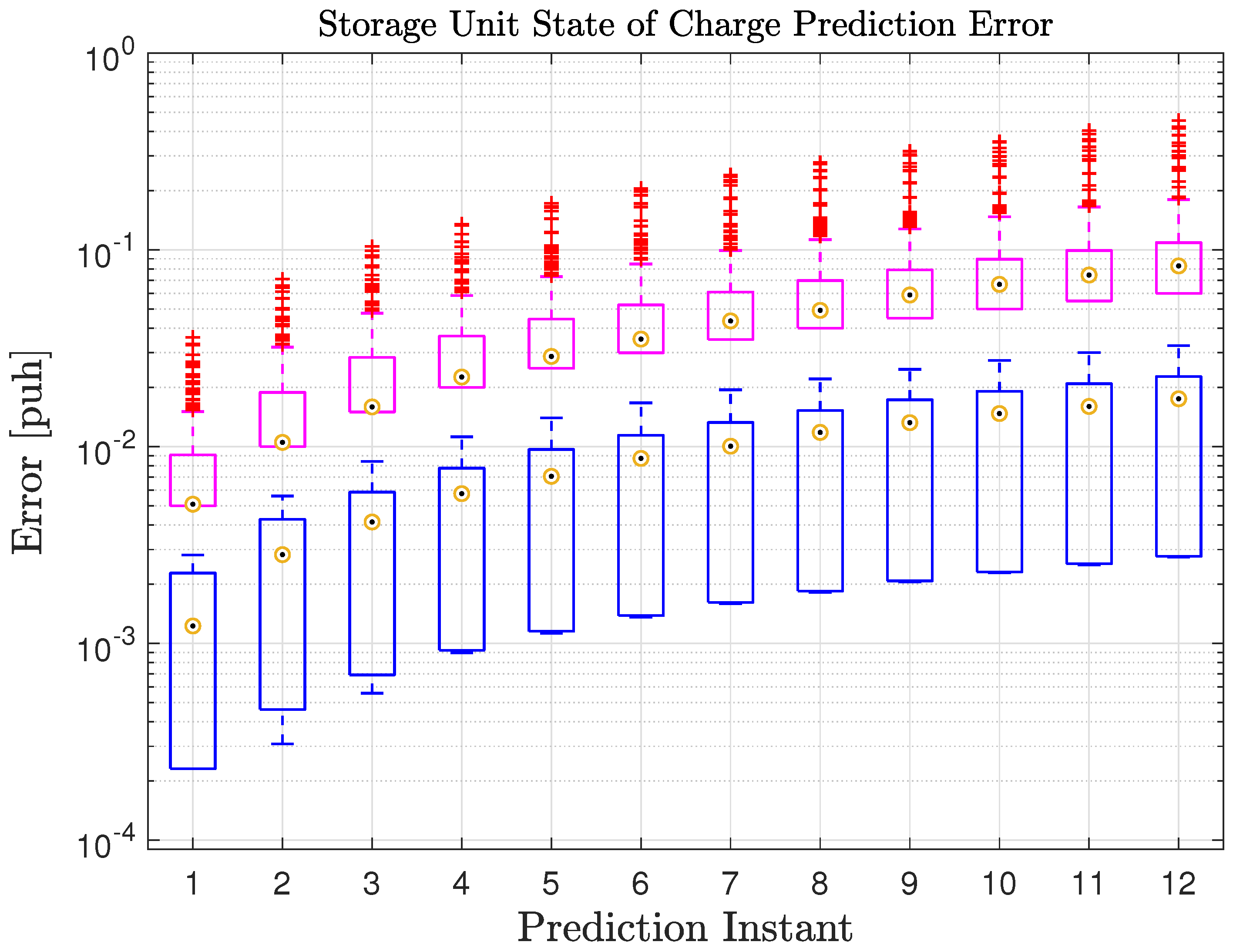
In accordance with Equations (25a), (25b) and (38), we chose ${\tilde{M}}_i=0.1$ and ${\tilde{m}}_i=-0.17$. We formulated the MPC problems in MATLAB using the YALMIP toolbox and solved them numerically with Gurobi. Here, we first compare the prediction error of the state of charge in the cases considering the dynamic storage with piecewise affine loss model (10)–(25) and the dynamic storage without piecewise affine loss model (26)–(29d) in the MPC problem. We formulated this error as $e\left(k\right)=x\left(k\right)-\tilde{x}\left(k\right)$, wherein $x\left(k\right)$ is the actual state of charge of the nonlinear loss model given the same power values, whereas $\tilde{x}\left(k\right)$ is the forecast of the state of charge. An analysis was carried out for both cases to compare the two cases. In the analysis, closed-loop simulations were performed over 366 simulation steps. For each simulation step, the state of charge prediction of the controllers (over 12 prediction steps) was compared to a prediction performed with the nonlinear plant model for the same storage power values. Then, at each prediction step, the probability distribution of the prediction errors was visualized in the form of box plots (see Figure 4). The circle of each box marks the median value of prediction errors of 336 data points in each prediction step. The box around the median values contains all data from the 25th to the 75th percentile. The downwards dash of each box represents the lowest occurring value of prediction error in each step, whereas the upwards dash marks the highest occurring value.

It can be seen in Figure 4 that, including the conversion losses in the proposed model predictive controller, the prediction error is reduced. For example, at $N=1$, when the conversion loss model is not employed in the controller, the median value is $5\times {10}^{-3}$. By adding the conversion loss model in the controller, this value is decreased 3 times to $1.5\times {10}^{-3}$. It is worth noting that this ratio increases as the prediction horizon rises. As can be observed from the last step of Figure 4, the median value of the error is equal to $9\times {10}^{-2}$ when the conversion loss model is not included in the controller, whereas this value is reduced to $2\times {10}^{-2}$ when the conversion loss model is added to MPC problem formulation. Therefore, the obtained results from Figure 4 illustrate that when we consider the dynamic storage with piecewise affine loss functions in the MPC problem, the actual state of charge $x\left(k\right)$ with much less error can be predicted by the controller.

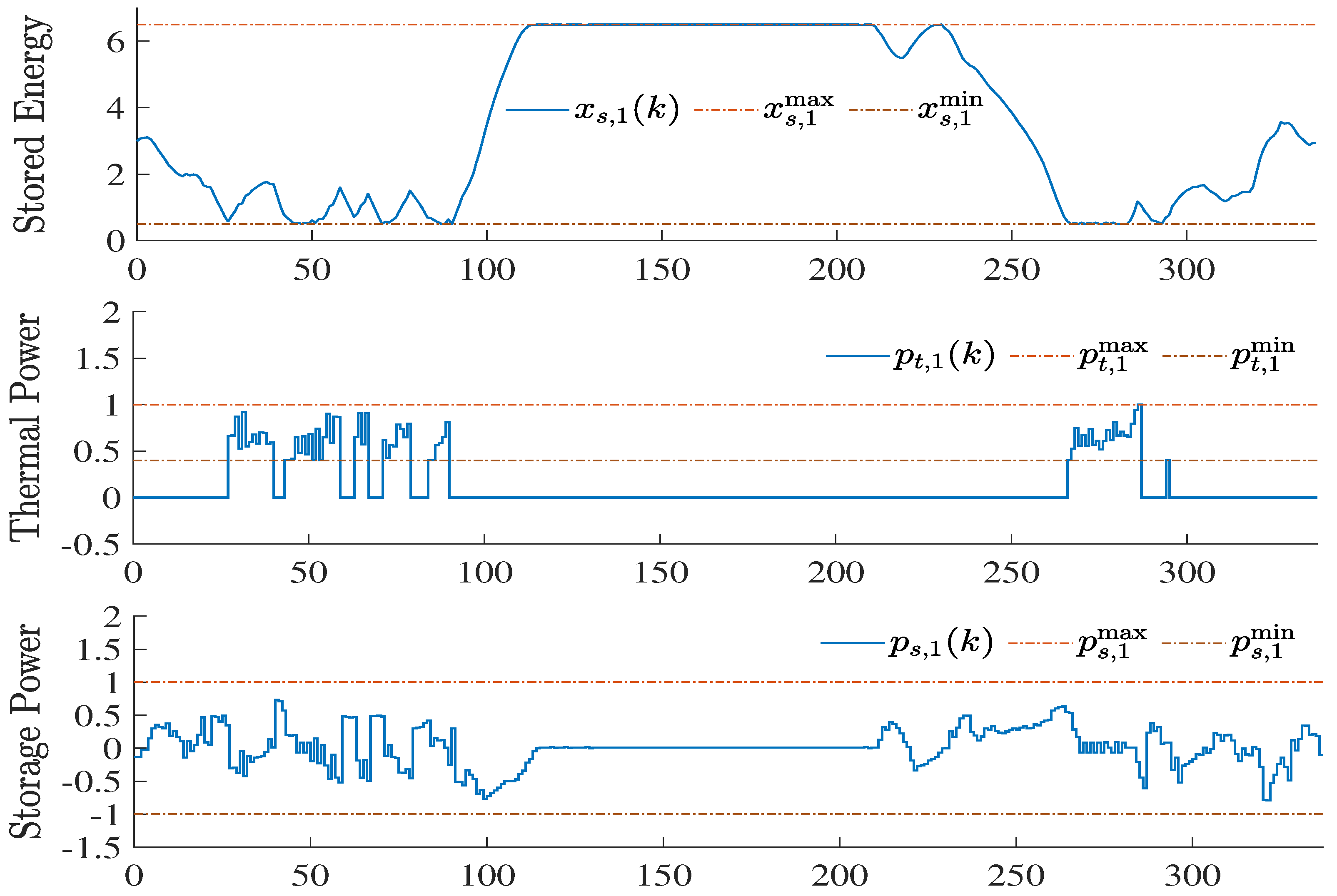
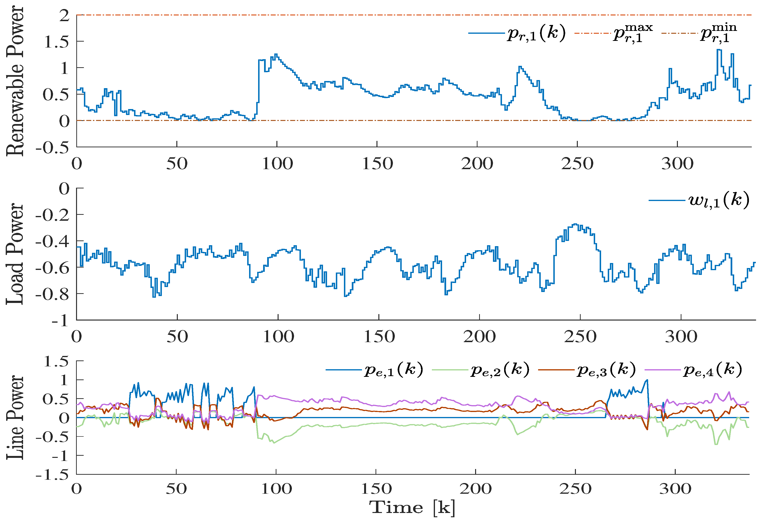
The closed-loop simulation results of the power of units and load, as well as the stored energy and line power of the MG, are depicted in Figure 5. It can be noted that, at the beginning of the period, since the available power of the renewable unit is low, the storage unit is discharging. When the battery is empty, the conventional generator is enabled to provide power to the load. As soon as the available power of the renewable unit is sufficient to provide power to the load, the conventional unit is disabled, and the storage unit is charged. When the stored energy reaches the upper end of the desired state of charge, the setpoint of the wind turbine is set such that the wind power only covers the load. Thus, the stored energy approximately remains at $x^{max}=6.5$ pu h. At some point, the available renewable unit power cannot entirely cover the load, and the storage is discharged. When the renewable unit reaches the minimum value $x^{min}=0.5$ pu h. and the storage unit is totally discharged, the conventional unit is activated again to provide power to the load. At the end of the simulation, the available power of the renewable unit increases again such that the storage unit can be charged with the available renewable unit power. These results indicate that the conventional units can be enabled and disabled during the simulation. Thus, the model is also able to work when RES and storage units are enabled. However, if the storage unit is discharged and the available power of the renewable unit is low, the conventional unit is repeatedly enabled to provide power to the loads and charge the storage units. Then, after increasing the available power of the renewable unit, the conventional unit is turned off. Hence, it results that by choosing this proposed operation control strategy, the share of power from RES can be significantly increased. Finally, it is clear from Figure 5 that the line power in the lower plot was within the given bounds of $\pm 1.3$ pu at all times.

6. Conclusions

In this work, we designed a novel certainty model predictive control approach for the operation of an islanded MG with a very high share of renewable energy sources. To this aim, a mathematical model of an islanded MG was derived by considering the conversion losses as quadratic functions to realistically model the scenario. In the model, we included (i) grid-forming storage units; (ii) renewable energy sources, where the power infeed can be limited, e.g., if storage units are fully charged; and (iii) conventional generators that can be disabled, e.g., in times of high available renewable infeed. Moreover, the model allowed us to approximately include the power flow over the transmission lines and a limitation thereof, as well as power-sharing of grid-forming units. In order to reduce the state of charge prediction error, we reformulated the conversion losses of storage units as piecewise affine functions and included them in the proposed controller. The obtained results confirmed that when considering the piecewise affine conversion loss functions in the proposed MPC, the prediction error of the state of charge decreased. Moreover, it is shown that the proposed scheme leads to a very high share of renewable energy sources in closed-loop simulations. Future works will investigate AC optimal power flow (OPF) problems, which are more realistic than the widely used linearized DC power flow approximations. To solve the AC OPF problems, we intend to employ a convex relaxation of the original problem, which leads to a second-order cone program (SOCP) that can be solved by available commercial software.

References

- Anderson, P.A.; Fouad, A.A. Power System Control and Stability; John Wiley and Sons: Hoboken, NJ, USA, 2003. [Google Scholar]
- Kundur, P.; Balu, N.J.; Lauby, M.G. Power System Stability and Control; McGraw-Hill: New York, NY, USA, 1994; Volume 7. [Google Scholar]
- Pehnt, M. Dynamic life cycle assessment (LCA) of renewable energy technologies. Renew. Energy 2006, 31, 55–71. [Google Scholar] [CrossRef]
- Peças, J.A.; Moreira, C.L.; Madureira, A.G. Defining control strategies for microgrids islanded operation. IEEE Trans. Power Syst. 2006, 21, 916–924. [Google Scholar]
- Hatziargyriou, N.; Asano, H.; Iravani, R.; Marnay, C. Microgrids. IEEE Power Energy Mag. 2007, 5, 78–94. [Google Scholar] [CrossRef]
- Gholami, M.; Pilloni, A.; Pisano, A.; Usai, E. Robust Distributed Secondary Voltage Restoration Control of AC Microgrids under Multiple Communication Delays. Energies 2021, 14, 1165. [Google Scholar] [CrossRef]
- Guerrero, J.M.; Vasquez, J.C.; Matas, J.; De Vicuña, L.G.; Castilla, M. Hierarchical control of droop-controlled AC and DC microgrids—A general approach toward standardization. IEEE Trans. Ind. Electron. 2011, 58, 158–172. [Google Scholar] [CrossRef]
- Guerrero, J.M.; Chandorkar, M.; Lee, T.L.; Chiang Loh, P. Advanced control architectures for intelligent microgrids—Part I: Decentralized and hierarchical control. IEEE Trans. Ind. Electron. 2012, 4, 1254–1262. [Google Scholar]
- Kanagawa, M.; Nakata, T. Assessment of access to electricity and the socio-economic impacts in rural areas of developing countries. Energy Policy 2008, 36, 2016–2029. [Google Scholar] [CrossRef]
- Barklund, E.; Pogaku, N.; Prodanovic, M.; Hernandez-Aramburo, C.; Green, T.C. Energy management in autonomous microgrid using stability-constrained droop control of inverters. IEEE Trans. Power Electron. 2008, 23, 2346–2352. [Google Scholar] [CrossRef] [Green Version]
- Logenthiran, T.; Srinivasan, D. Short term generation scheduling of a microgrid. In Proceedings of the TENCON 2009—2009 IEEE Region 10 Conference, Singapore, 23–26 January 2009; pp. 1–6. [Google Scholar]
- Chen, C.; Duan, S.; Cai, T.; Liu, B.; Hu, G. Smart energy management system for optimal microgrid economic operation. IET Renew. Power Gener. 2011, 5, 258–267. [Google Scholar] [CrossRef]
- Palma-Behnke, R.; Benavides, C.; Lanas, F.; Sev, B.; Reyes, L.; Llanos, J.; Sáez, D. A microgrid energy management system based on the rolling horizon strategy. IEEE Trans. Smart Grid 2013, 4, 996–1006. [Google Scholar] [CrossRef] [Green Version]
- Heymann, B.; Bonnans, J.F.; Martinon, P.; Silva, F.J.; Lanas, F.; Guillermo, J.E. Continuous optimal control approaches to microgrid energy management. Energy Syst. 2018, 9, 59–77. [Google Scholar] [CrossRef] [Green Version]
- Mayhorn, E.; Kalsi, K.; Elizondo, M.; Zhang, W.; Lu, S.; Samaan, N.; Butler-Purry, K. Optimal control of distributed energy resources using model predictive control. In Proceedings of the 2012 IEEE Power and Energy Society General Meeting, San Diego, CA, USA, 22–26 July 2012; pp. 1–8. [Google Scholar]
- Olivares, D.E.; Cañizares, C.A.; Kazerani, M. A centralized energy management system for isolated microgrids. IEEE Trans. Smart Grid 2014, 5, 1864–1875. [Google Scholar] [CrossRef]
- Hans, C.A.; Nenchev, V.; Raisch, J.; ReinckeCollon, C. Minimax model predictive operation control of microgrids. IFACProceedings 2014, 47, 10287–10292. [Google Scholar] [CrossRef] [Green Version]
- Sui, Q.; Wei, F.; Wu, C.; Lin, X.; Li, Z. Day-Ahead Energy Management for Pelagic Island Microgrid Groups Considering Non-Integer-Hour Energy Transmission. IEEE Trans. Smart Grid 2020, 11, 5249–5259. [Google Scholar] [CrossRef]
- Tran, Q.T.T.; Riva Sanseverino, E.; Zizzo, G.; Di Silvestre, M.L.; Nguyen, T.L.; Tran, Q.-T. Real-Time Minimization Power Losses by Driven Primary Regulation in Islanded Microgrids. Energies 2020, 13, 451. [Google Scholar] [CrossRef] [Green Version]
- Nair, U.R.; Costa-Castelló, R. A Model Predictive Control-Based Energy Management Scheme for Hybrid Storage System in Islanded Microgrids. IEEE Access 2020, 8, 97809–97822. [Google Scholar] [CrossRef]
- Zia, M.F.; Elbouchikhi, E.; Benbouzid, M.; Guerrero, J.M. Energy Management System for an Islanded Microgrid with Convex Relaxation. IEEE Trans. Ind. Appl. 2019, 55, 7175–7185. [Google Scholar] [CrossRef]
- Hans, C.A.; Sopasakis, P.; Raisch, J.; Reincke-Collon, C.; Patrinos, P. Risk-averse model predictive operation control of islanded microgrids. IEEE Trans. Control Syst. Technol. 2020, 28, 2136–2151. [Google Scholar] [CrossRef] [Green Version]
- Lei, J.; Hans, C.A.; Sopasakis, P. Optimal operation of microgrids with risk-constrained state of charge. arXiv 2021, arXiv:2104.08357. [Google Scholar]
- Hans, C.A.; Braun, P.; Raisch, J.; Grüne, L.; Reincke-Collon, C.R. Hierarchical distributed model predictive control of interconnected microgrids. IEEE Trans. Sustain. Energy 2019, 10, 407–416. [Google Scholar] [CrossRef] [Green Version]
- Sampathirao, A.K.; Hofmann, S.; Raisch, J.; Hans, C.A. Distributed Conditional Cooperation Model Predictive Control of Interconnected Microgrids. arXiv 2021, arXiv:1810.03361v2[cs.SY]. [Google Scholar]
- Gholami, M.; Pisano, A.; Usai, E. Robust Distributed Optimal Secondary Voltage Control in Islanded Microgrids with Time-Varying Multiple Delays. In Proceedings of the 2020 IEEE 21st Workshop on Control and Modeling for Power Electronics (COMPEL), Aalborg, Denmark, 9–12 November 2020; pp. 1–8. [Google Scholar]
- Pilloni, A.; Gholami, M.; Pisano, A.; Usai, E. On the robust distributed secondary control of islanded inverter-based microgrids. In Variable-Structure Systems and Sliding-Mode Control; Springer: Cham, Switzerland, 2020; pp. 309–357. [Google Scholar]
- Purchala, K.; Meeus, L.; Van Dommelen, D.; Belmans, R. Usefulness of DC power flow for active power flow analysis. In Proceedings of the IEEE Power Engineering Society General Meeting, San Francisco, CA, USA, 16 June 2005; pp. 454–459. [Google Scholar]
- Krishna, A.; Hans, C.A.; Schiffer, J.; Raisch, J.; Kral, T. Steady state evaluation of distributed secondary frequency control strategies for microgrids in the presence of clock drifts. In Proceedings of the 2017 25th Mediterranean Conference on Control and Automation (MED), Valletta, Malta, 3–6 July 2017; pp. 508–515. [Google Scholar]
- Bemporad, A.; Morari, M. Control of systems integrating logic, dynamics, and constraints. Automatica 1999, 35, 407–427. [Google Scholar] [CrossRef]
- Petrollese, M.; Valverde, L.; Cocco, D.; Cau, G.; Guerr, J. Real-time integration of optimal generation scheduling with MPC for the energy management of a renewable hydrogen-based microgrid. Appl. Energy 2016, 166, 96–106. [Google Scholar] [CrossRef]
- Zivic Djurovic, M.; Milacic, A.; Krsulja, M. A simplified model of quadratic cost function for thermal generators. In Proceedings of the 23rd International DAAAM Symposium, Zadar, Croatia, 24–27 October 2012; Volume 23, pp. 25–28. [Google Scholar]
- Vetter, J.; Novak, P.; Wagner, M.R.; Veit, C.; Moller, K.-C.; Besenhard, J.; Winter, M.; Wohlfahrt-Mehrens, M.; Vogler, C.; Hammouche, A. Ageing mechanisms in lithium-ion batteries. J. Power Sources 2005, 147, 269–281. [Google Scholar] [CrossRef]
Figure 1.
Certainty equivalence MPC scheme for operation of islanded MG at time instant k and .
Figure 2.
MG used for operation control as a running example.
Figure 3.
Control scheme of certainty equivalence MPC under the conversion loss functions.
Figure 4.
The prediction error of the state of charge (Up) with the dynamic storage without piecewise affine loss model (26)–(29d) in the controller; (Down) with the dynamic storage with piecewise affine loss model (10)–(25) in the controller.
Figure 5.
Power of units and load.