Abstract
Simultaneous real-time monitoring of measurement and parameter gross errors poses a great challenge to distribution system state estimation due to usually low measurement redundancy. This paper presents a gross error analysis framework, employing PMUs to decouple the error analysis of measurements and parameters. When a recent measurement scan from SCADA RTUs and smart meters is available, gross error analysis of measurements is performed as a post-processing step of non-linear DSSE (NLSE). In between scans of SCADA and AMI measurements, a linear state estimator (LSE) using PMU measurements and linearized SCADA and AMI measurements is used to detect parameter data changes caused by the operation of Volt/Var controls. For every execution of the LSE, the variance of the unsynchronized measurements is updated according to the uncertainty introduced by load dynamics, which are modeled as an Ornstein–Uhlenbeck random process. The update of variance of unsynchronized measurements can avoid the wrong detection of errors and can model the trustworthiness of outdated or obsolete data. When new SCADA and AMI measurements arrive, the LSE provides added redundancy to the NLSE through synthetic measurements. The presented framework was tested on a 13-bus test system. Test results highlight that the LSE and NLSE processes successfully work together to analyze bad data for both measurements and parameters.
1. Introduction
The introduction of distributed energy resources (DER) presents further technical challenges besides the obvious advantages. The dynamics of the distribution systems operation are becoming more complicated with fluctuating voltages and power flows. These adverse impacts impose technical challenges to distribution management systems (DMS) and micro phasor measurements units (PMUs) are the perfect tool to address these new challenges [1]. Algorithms for adequately estimation of synchrophasors in distribution systems have specific properties, such as rejection of harmonics and steady uncertainty values under transients [2].
The importance of having real-time, accurate monitoring processes and constant situational awareness in any power system cannot be overstated. State estimation (SE) is a fundamental process for real-time monitoring of the power system. Distribution system state estimation (DSSE) especially has its own share of technical difficulties. The low availability of measurements is a huge burden on its reliability. This can cause the system to be unobservable, thus making a full state estimate infeasible [3,4]. Even if the system is observable, a lack of measurement redundancy increases vulnerability of its state estimate to bad data [5]. A popular method of ensuring the observability or adding redundancy to a system’s measurement set is the use of pseudo-measurements. Pseudo-measurements are estimates, or forecasts, of measurements based on historical data. The extrapolation of pseudo-measurements using past data or their interpolation when forecast of load or generation is available has been proposed to capture the trend in which measurements evolve over time to improve the accuracy of pseudo-measurements [6]. It has been shown that, since these are less accurate than real-time measurements, they can introduce errors to the state estimate [7,8].
Voltage fluctuations due to the intermittent nature of the DER have a direct effect on the operation of Volt/Var control (VVC) schemes, which actuate capacitor banks and linear tap changers (LTCs) in order to maintain voltage within American National Standards Institute (ANSI) limits. In a scenario where measurements are scarce, as in DSSE, additional parameter variations due to VVC actions not reported to the DMS represent yet another technical challenge for accurate real-time monitoring of distributions systems. The current inclusion of advanced metering infrastructure (AMI), such as smart meters, in the distribution system will increase measurement redundancy level. PMU-based systems are a candidate solution for monitoring VVC changes and there are applications of these systems for event detection in distributed systems [9]. Recently, an experiment has shown that PMUs can be used to identify capacitor bank operations in a real-life distribution feeder using both steady-state and transient synchrophasor data analysis [10].
Unlike GPS-synchronized measurements produced by PMUs, SCADA, and AMI scans are taken in different points in time, which means that each measurement provides a piece of information with a different time-delay. Characterizing the statistics of consecutive time scans as a Gaussian independent process for each meter and using linear interpolations to obtain their expected mean and variance has been presented as a solution to the problem of processing unsynchronized measurements [11]. However, while we can assume that the Gaussian noise in measurement process might be uncorrelated, it is not possible to assert that the changes in state and load variations captured by any two meters are independent.
Tracking state estimation for distribution systems using compensation theorem has been proposed to incorporate synchrophasor measurements to slow-scale DSSE by updating the states following the detection of an important change in an element of the system [12]. The iterated Kalman filter (IKF) has been proposed for performing state estimation in active distribution networks [13].
This paper presents a method of using PMU data in DSSE which incorporates a linear DSSE to decouple the gross error analysis for measurements and parameters. Added redundancy improves measurement gross error detection and identification through while detecting parameter changes on the system between SCADA and AMI scans. Unlike dynamic state estimators, this method does not require the estimation of additional states present in dynamic state estimation, such as frequency [14,15], nor does it assume constant impedance load models [14]. Furthermore, during most of the process, the estimator does not require time-consuming iterative processes, unlike, for example, traditional non-linear (including tracking) state estimators or IKF [13]. This method presents two specific contributions towards the state of the art:
- The decoupling of gross error analysis in measurements and parameters in two different time scales: a slow time scale for processing gross errors in measurements and a fast time scale for gross error analysis in parameters due to operation of VVC;
- The use of unsynchronized and linearized SCADA measurements with load model-based temporal update of uncertainty combined with PMU measurements for DSSE.
The remainder of this paper is organized as follows. Section 2 presents the PMU based framework for DSSE gross error analysis. Section 3 presents the modified non-linear state estimation model. Section 4 presents the modified linear state estimation model. Section 5 presents a case study. Conclusions of this work are presented in Section 6.
2. PMU-Enhanced DSSE Gross Error Analysis
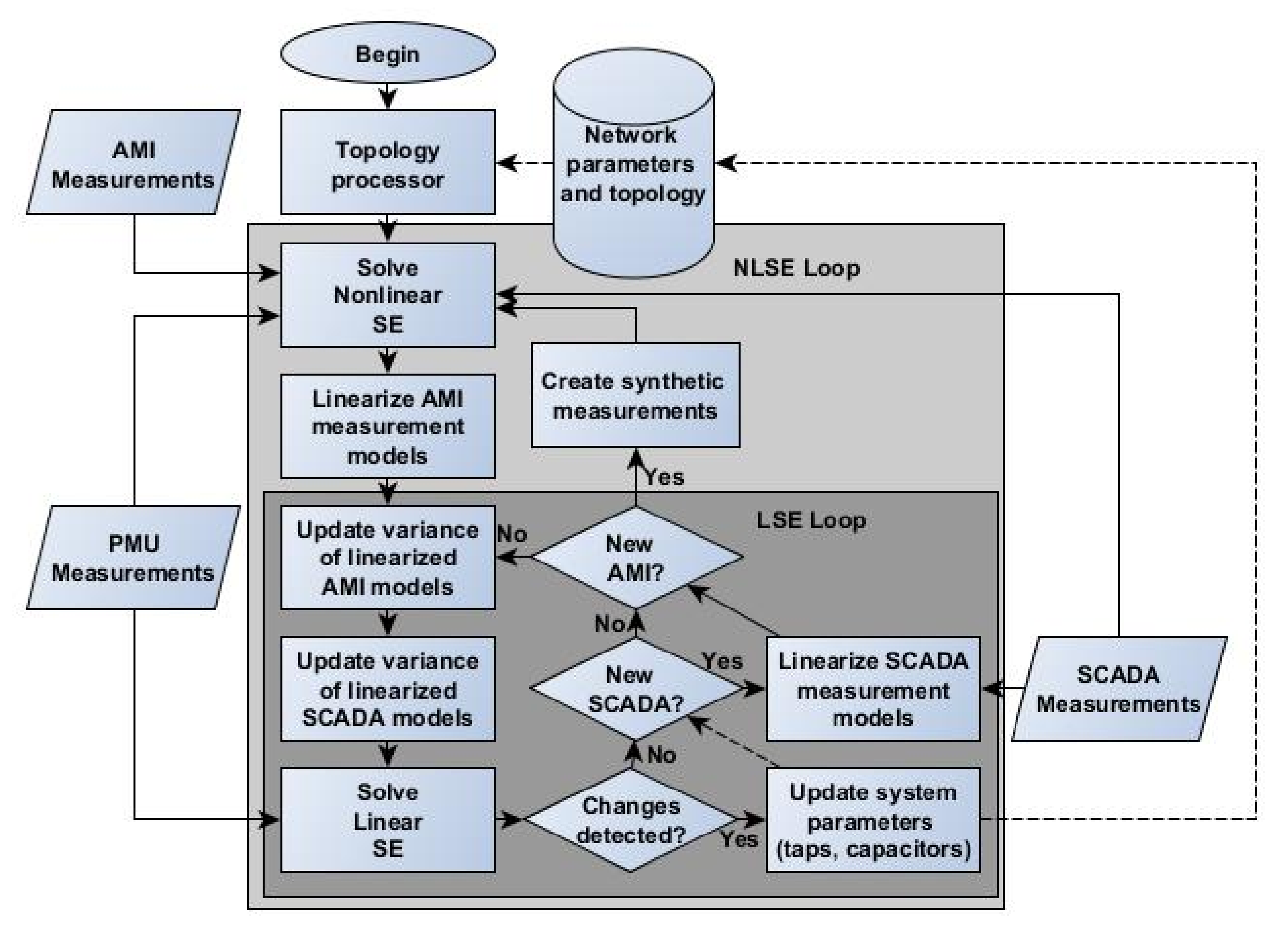
Assuming that the parameters of the devices (e.g., line and transformer parameters) in a distribution system are known at a given point in time, then the process of gross error analysis is narrowed down to the identification of bad data in measurements and, with respect to parameters, in the position of LTCs and capacitor banks. If those assumptions hold true, then bad data analysis requires far less redundancy than if simultaneous estimation of parameters and states is performed. The idea of decoupling gross errors analysis of measurements and parameters is thus most appropriate. Considering such, we present an on-line DSSE gross error analysis framework composed of two loops: the linear state estimation loop (LSE) and the non-linear state estimation loop (NLSE). An overview of the presented method is shown in Figure 1.
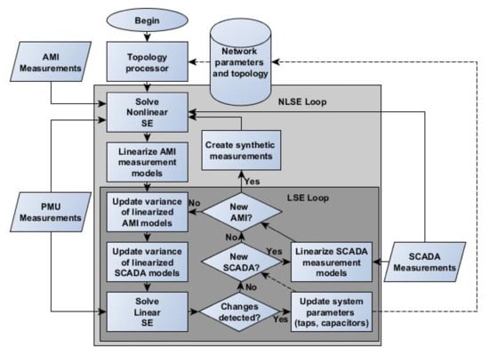
Figure 1.
Flowchart showing the PMU-Enhanced DSSE gross error analysis method.
The goal of NLSE is to perform gross error analysis in measurements when the maximum level of redundancy is available, i.e., when recent SCADA, AMI, PMU, and synthetic measurements (SM) [16] are available. Although PMUs are capable of taking 120 phasor measurements per second [17], SCADA systems can poll measurements from RTUs in a smaller sampling rate, every 2–4 s [6]. In this paper, we make a more conservative consideration and assume that new SCADA readings are available every 1 min [18]. AMI measurements are usually obtained every 15 min [6]. Currently, most utilities only collect smart meter data once or twice a day [19], however we envision that in the near future this data-rate might increase and it will be possible to obtain measurements every 15 min [6,20].
The objective of the LSE loop is to take advantage of the high sampling rate and accuracy of PMU measurements to detect the operation of the VVC devices, identify the parameter that has changed and update system parameters accordingly. Given that proper gross error analysis in parameters is performed by the LSE, accurate bad data processing in measurements is possible for the NLSE.
Identifying the changed parameter accurately is a challenging task because any VVC operation will instantaneously change the state of the system and consequently the SCADA or AMI measurements will become obsolete. To make this detection possible, we will consider that the feeder has at least two PMUs: one in the substation and the other anywhere downstream of the LTC. Additionally, both capacitor banks and LTC have discrete states, an information that the state estimator will use to perform the correction properly.
The process of DSSE starts with a flat start and the topology processing so that a bus-branch model of the distribution system is obtained. As soon as the SCADA system receives the most recent batch of measurements from the distribution feeder, the latest PMU data are collected and NLSE is performed. SM are only included after the first NLSE iteration. Once NLSE converges, innovation-based error detection is performed to detect gross errors in measurements [21]. It should be clear that other parameter errors are possible, as of devices. This condition though is not considered in this work.
3. Non-Linear State Estimation
The NLSE follows the traditional formulation of the SE problem, represented by the set of non-linear equations, (1).
where is the measurement vector, is the state variables vector, is a continuously non-linear differentiable function, is the measurement error vector assumed having zero mean and Gaussian probability distribution and covariance . is the number of unknown state variables to be estimated (n is the number of electrical nodes in the network). The measurements are composed by three sets of data: AMI, SCADA, and PMU. The set of AMI measurements is composed of aggregated real and reactive bus power injections and estimated bus voltage magnitudes, obtained at a very slow sampling rate, in the order of 15 min. SCADA measurements include power flows, injections and voltage magnitudes obtained once every minute. Bus voltage phasors along with branch current flow and bus current injection phasor measurements are obtained at a very fast sampling rate through PMUs.
The problem of NLSE is set as a weighted least-squares state estimation problem as described in [22]. It is in an optimization problem where we want to find the optimal value of the states, , that minimizes the weighted sum of the squares of the residuals, defined as the difference between the measurements and the measurement function, divided by the standard deviation. This problem is described by (2).
where the objective function can be represented as . The NLSE problem solved using the Gauss–Newton algorithm [22]. Starting from an initial guess for the solution, this algorithm iteratively solves the non-linear set of equations by successfully linearizing the equations, (3), at a point of operation, , and solving the resulting linear system (4) and (5). Once a solution to each linearized problem is obtained, the incumbent solution is updated by the state correction vector, , where the equations are linearized again. The process is repeated until a very small is obtained, implying that the first-order optimality condition is met and an optimal solution was found.
where is the Jacobian matrix, is the gain matrix and is the weight matrix. The vector of state correction is obtained by solving (6). The vector of states updated according to (7).
It is important to note that the NLSE presented in [22] includes only measurement models for SCADA and AMI type measurements. In order to include the current measurements obtained by PMUs as well, Method 2 from [23] is adapted in this paper’s NLSE measurement models. The procedure for bad data analysis follows [21,24,25,26].
4. Linear State Estimation
In between NLSE iterations, on-line system monitoring is performed by the LSE. The goal is to leverage the high granularity of the PMU measurements to detect and identify changes in parameters due to VVC operation, so that when the next batch of SCADA and AMI measurements is available, the system parameters are up-to-date. Due to the higher sampling rate of PMUs, an iterative state estimation algorithm is ill-suited to solve the problem of state estimation because of the very short time in which the SE problem must be solved and bad data be processed. The solution is then to speed-up the solution by linearizing the problem, thus enabling LSE that can be solved directly with no need for iterations.To maximize redundancy and avoid unobservability, SCADA, AMI, and PMU data are used simultaneously as inputs to LSE. Therefore, a linearization of non-linear SCADA and AMI measurement functions is necessary.
The first step is to linearize the non-linear SCADA and AMI measurement model components, such as voltage magnitudes, power flows, and injections, by transforming them into current phasors of voltage, flows, and injections, respectively, based on the results of the NLSE. The LSE is composed by two parts: the purely PMU-based estimation, top equations of (8), and the linearized estimation of unsynchronized AMI and SCADA measurements, bottom equations of (8). The solution of this system of equations will be explained on Section 4.4.
where the vector of states is given by , the measurement set of the linearized part is composed of branch current flows, , bus current injections, , and bus voltages, , and is given by for unsynchronized measurements. Similarly, the set of PMU measurements, , is composed of current flows and injections and voltage measurements, respectively, represented as , where is the total number of PMU measurements.
4.1. Linearization of Unsynchronized Measurements
To linearize the system of equations, it is necessary to obtain the equations that relate the linear and non-linear measurement models. For , which represents the linearized measurements of voltage phasors, it is necessary to replace the vector of voltage magnitude measurements from NLSE in LSE, such that , where is the estimated angle of the voltage phasor and and are, respectively, its real and imaginary components [27]. represents the linearized measurements of current injection phasors that replace the complex power injection measurements, , for real bus power injections and reactive power injections . To do so, it is necessary to calculate the current injections as , where is the estimated bus voltage phasor obtained by the NLSE and is the complex power injected in bus i. represent the linearized measurements of current flow phasors that replace the complex branch power flows from NLSE in LSE, such that [28]. Both current injection and flow can be linearized as (9).
where and can be power injections or flows from bus i to a neighboring bus. Since some of these transformations are non-linear, the calculation of the covariances of these linearized measurements will be approximated using the truncated Taylor expansion of their functions. Let us first define the i-th vector of linearized real and imaginary parts of currents as and the independent variables as . Let and . Then, the Taylor series expansion can be represented by (10).
where is the Jacobian of (9) with respect to . The variance can be calculated using the same expansion as (11).
The variance and covariance elements of and can be extracted from the covariance matrix of the estimated states, (if rectangular coordinates for states are used) and the covariances between the states and measurements can be obtained from the covariance matrix . The variance of the current is given by (12).
4.2. Load Model as an Ornstein–Uhlenbeck Stochastic Process
As time passes, the linearized SCADA and AMI measurements become obsolete because of load dynamics and eventual changes in parameters. Although the goal of LSE is to process the gross errors in parameters, the load-induced errors introduced in outdated unsynchronized measurements must be considered. We can model this drift of the system state as a stochastic process. In the literature, time-variations of loads have been successfully represented as Ornstein–Uhlenbeck (OU) random processes [29,30], which is a mean-reverting stochastic process. The rationale behind this modeling is based on the assumption that the aggregated loads are expected to fluctuate in the short-term, but it is very unlikely that they will largely deviate from their previous estimate. Given that the variance of the measurements and change in the state can be modeled as an OU process, we can use this information to update the uncertainty of LSE measurements according to the model of the random process. To illustrate this idea, Figure 2 shows the comparison of an unsynchronized current measurement taken at s from the test system in Figure 4 with its true value. With the loads modeled as an OU process, we can see that very frequently these load variations might cause the true value to deviate from the unsynchronized measurement by more than 3 standard deviations. Consequently, as time passes, the standard deviation of the measurement error is no longer an adequate measure of the uncertainty associated with the measurement. To improve the quantification of uncertainty, we present a method for updating the standard deviation of measurements based on the OU process models of the loads.

Figure 2.
Unsynchronized measurement taken at s and the load-induced drift of its true value over time.
The load current, , can be represented by the stochastic differential Equation (13) [31].
where , is a complex Wiener process with normally distributed increments, is the size of the noise and is the decay rate for . These parameters can be estimated by measuring the statistics of PMU readings [30]. Assuming that the mean variation in the load current is expected to be zero and that , then the solution (13) is (14) [31].
where is the time instant when the SCADA or AMI unsynchronized measurement was relayed. If we now consider that the PMUs will sample data every seconds, we can treat the load variations as a time-sampled process, where and , where k and q are time step indexes.
where is a complex random variable with mean zero and variance . The expected value of the Gaussian time-discretized variable is zero and its variance is given directly by (16) [32] or recursively by (17).
where .
The increment in consumption between time and time k of the loads is represented by the vector of current injections . The variance of these currents will be calculated according to (12) if the corresponding current is measured by AMI or SCADA. If the current is measured directly by a PMU, then its variance can be estimated as equal to the variance of its measurement. If the load current connected to the v-th bus is not measured, then its value, , will be estimated based on the system parameters and estimated states according to (18).
where is the v-th row of the bus admittance matrix.
4.3. Load Dynamics-Induced Measurement Uncertainty
Now let us consider that the true value (with no noise) of any i-th measurement, , at a given time instant k is related with a previous value, , plus the random variation over time , as represented by (19), while its unsynchronized and outdated noisy reading, , is given by (20).
where models the noise of the measurement, assumed to be additive Gaussian. When performing LSE at instant k, the value of interest is , but its exact value is unknown and the closest information available is . If we assume that is exclusively induced by load variations and its model parameters can be estimated, then it is possible to approximate the expected value of by (21).
This model is considered when estimating the value of unsynchronized measurements and their variance. The initial value of is obtained from the NLSE. Taking this simple model to the concrete case of LSE, we can represent the vector of unknown measurements as (22) in the same way as (21) by considering that the closest we have to the true values is the known outdated vector of measurements and their deviations are functions of the load variations , given by the added measurement uncertainty.
where is the admittance matrix that is used to calculate the current flows and is the bus impedance matrix. Following (8) the variance of is given by (24).
where and .
4.4. Derivation of LSE: Maximum Likelihood Estimation
For LSE, there are two types of zero-mean Gaussian random variables, and . Let the probability density function of the random vectors and be defined as . Since and are independent, we can rewrite the expressions as . By replacing the errors by the terms in (8) we have the likelihood functions of circular complex-valued Gaussian random variables [33]:
where is the vector of residuals of PMU measurements.
is the vector of residuals of unsynchronized measurements. The only unknown is the vector of states, . Using a maximum likelihood estimation approach, we can set the problem as (27).
4.5. Analysis of Parameter Errors Due to Switching Events
Variations in parameters change , which will lead to an increase in the values of the residuals of the LSE estimation. The chi-squared () test is used to detect errors in the estimation. For the sake of simplicity, we approximate the value of as equal to the objective function of (29) and the number of degrees of freedom as .
When an error is detected, it is assumed that any gross errors in measurements were already adequately processed by the NLSE. Therefore, we consider that no gross errors in measurements exist and the causes of parameter errors will be assumed to be capacitor banks and LTCs. Since a feeder might have more than one capacitor bank and possibly more than one tap changer, the first step in the identification process is to narrow down the possible parameter changes. To do that, the PMU downstream of the LTC is used to detect if the voltage has increased or decreased. For instance, if the voltage has increased, then the possibility of an LTC operation that decreased the turns ratio or capacitor banks switching off are discarded. To make a difference between a capacitor change and a LTC operation, the reactive power flow out of the substation is used. If the reactive power flow has changed in a value that is close to the value of the capacitor bank, then the capacitor bank operation is likely to have caused the change in voltage. Otherwise, the LTC is the probable suspect. This error processing is summarized in Figure 3.
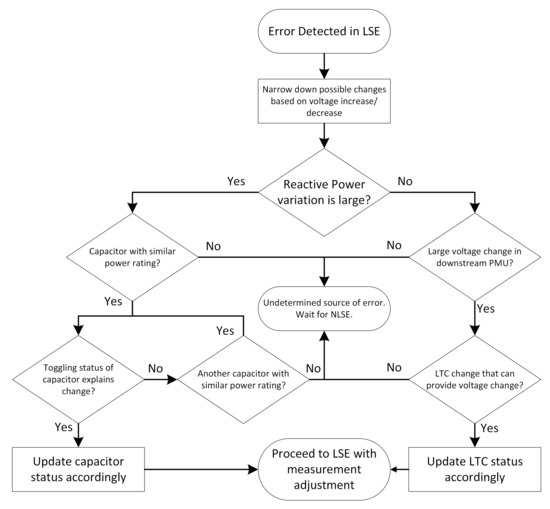
Figure 3.
Flowchart for parameter error processing.
A likelihood ratio test is then used to verify the correctness of the identification of the parameter error. The likelihood function of the estimated states can be calculated by multiplying (25) and (26) evaluated at the estimated state, . To obtain the likelihood of the alternative hypothesis, i.e., that one parameter has changed, a new state estimation is performed with the alternative parameters of the system and then, with the result of this new SE, the likelihood function is calculated.
where is the original and is the alternative set of parameters. The latter contains the candidate value for LTC turns ratio or state of capacitor bank. The null hypothesis is accepted is larger than one. Otherwise, the alternative hypothesis is accepted and the parameters are updated. In both cases, the SCADA and AMI measurements have to be updated. Their outdated value is replaced by the evaluation of the measurement function at the estimated state, .
4.6. Synthetic Measurements
Finally, when a new batch of SCADA and AMI measurements is available [34], SM are created and added to the measurement set for the NLSE, which has been shown to be effective in [35]. SM are calculated based on the previously set of state estimates and the current system parameters. The location and type of SM created by the LSE are strategically chosen based on the VI of a given bus i (33).
where K is the set of measurements associated with bus i, J is the set of all measurements.
and are the sensitivities of the composed measurement error (CME) [21,25,26] and residual, respectively, with respect to gross errors in measurements. The VI identifies buses that are most vulnerable to undetectable errors, as shown in [16]. Adding redundancy via SM will cause the residuals (and CMEs) to have a more Gaussian behavior, thereby improving the reliability of the gross error detection test. As opposed to the commonly used pseudo-measurements, SM are calculated from the current state of the system, making them more appropriate for real-time monitoring.
5. Numerical Tests
Parameter Error Processing
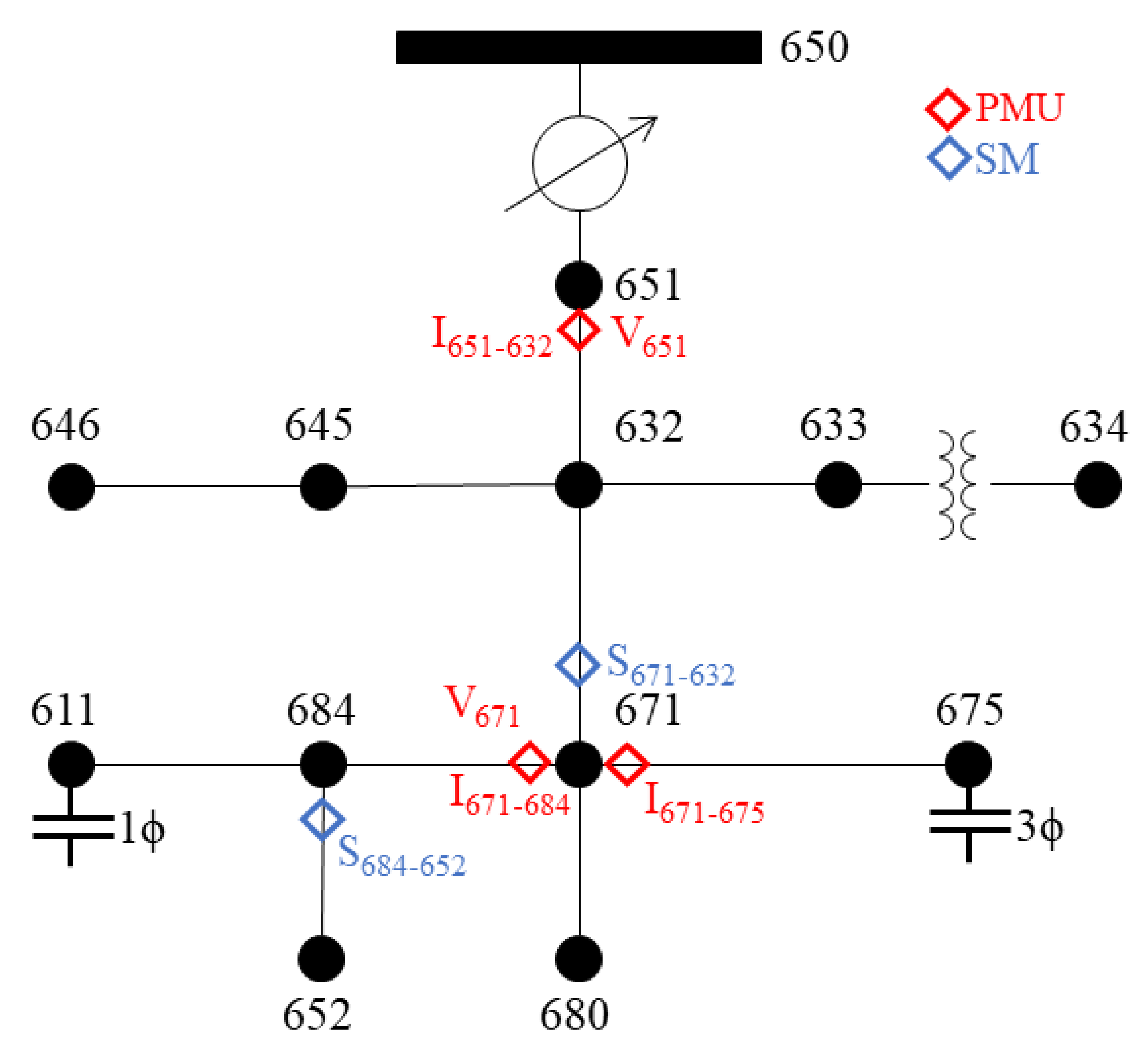
To evaluate the effectiveness of the parameter error detection approach, a test is performed in a modified version of the IEEE 13-bus test distribution system shown in Figure 4. Initially, a NLSE is performed at s and after that LSE monitors the parameter variations. We consider that the error of the unsynchronized voltage magnitude measurements is within of the reading and for the power measurements is . For PMU measurements, the error is smaller than of the value of the measurement [17]. The standard deviation of the noise of each measurement is considered as one third of its error. The parameter is equal to as obtained by [30] and for all loads is equal to of the magnitude of the load, also similar to the values obtained in the distribution of PMU data [30]. The turns-ratio of the LTC change at of the rated voltage at each tap operation [36] and the capacitor bank power outputs at rated voltage is p.u. at bus 675 and p.u. at bus 611. The simulation is performed in MATLAB with a time-step of 100 ms, a slower rate than the PMU’s maximum capability, so there is time available for the LSE to finish before new readings are available. The results shown are from a 15-min window with multiple VVC events.
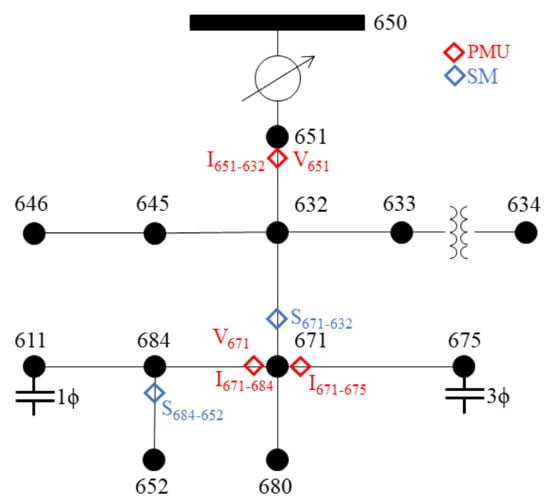
Figure 4.
Test system for parameter detection and identification test.
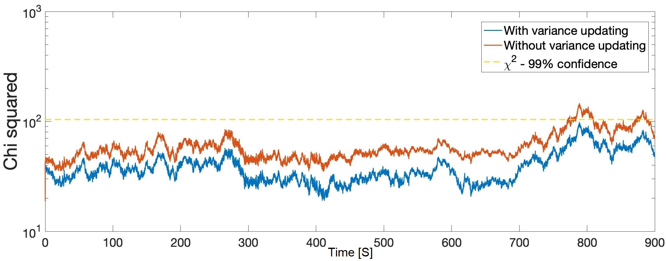
Figure 5 shows that during the simulation the standard deviation of voltage and current measurements based on linearized unsynchronized measurements are updated at every time step. As a consequence, with smaller weights, larger deviations from the estimated state tend to be less penalized by the estimator. That avoids the false positives in the error detection phase. A comparison of values of two instances of the LSE, one with update of variance (blue curve) and the other one not (orange curve), is shown in Figure 6. In this test, no VVC operations are performed and the LSE only suffers perturbations from load variations and measurement noise. In the case where the variance of all measurements is held constant there are multiple false detections of VVC operations. When the variance of measurements is corrected, the value of is always lower than the detection threshold with 73 degrees of freedom and a confidence level of .

Figure 5.
Variance of measurements when variance update is applied.

Figure 6.
Comparison of Chi-Squared tests when the update of variance of measurements is applied (blue) or kept constant (orange).
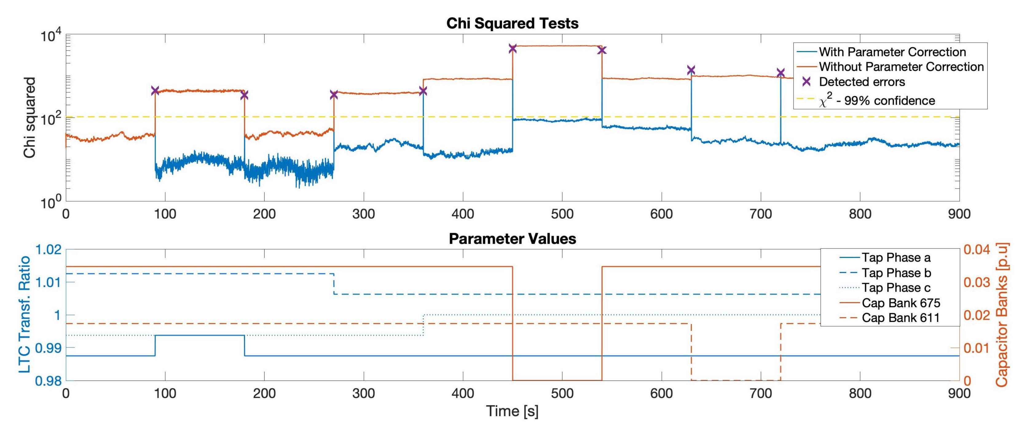
In order to test the framework’s effectiveness, a sequence of VVC operations occurs, as shown in the bottom plot of Figure 7. At s the tap position of phase a changes, increasing the turns ratio of the LTC, then it returns to the previous position at s. The turns ratio at phase b is decreased at s and the turns ratio at phase c is increased at s. The capacitor bank at bus 675 is switched off at s and is switched back on at s. Finally, the capacitor bank at bus 611 is switched off at and back on at . As we can see on Figure 7, in all cases when there is a change in the parameters of the system, the value of becomes significantly larger than the threshold. That is clearly shown by the orange line in the top plot, which show values obtained when no parameter is corrected.
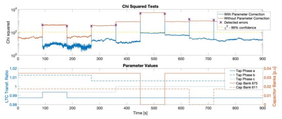
Figure 7.
Chi-square value (top) and turns-ratio of LTC and value of capacitor banks (bottom).
If we apply the method for parameter error detection and identification, we obtain the blue curve in Figure 7. The purple crosses in the same figure indicate the value of obtained when errors were detected for the case where parameter correction occurs. We can notice that all parameter errors can be detected and identified correctly with the proposed method. The mean time to perform the LSE algorithm and the bad data processing routine in MATLAB was 7.4 ms and the maximum time was 33.2 ms. This result shows that, in this case, the LSE could be run 3 times as often as it is in this test. During all of the 8 switching events, the likelihood ratio gave very low results, in the order of or lower. Such low values indicate the very clear distinction between the likelihood of the two hypotheses, obtained due to the use of two PMUs.
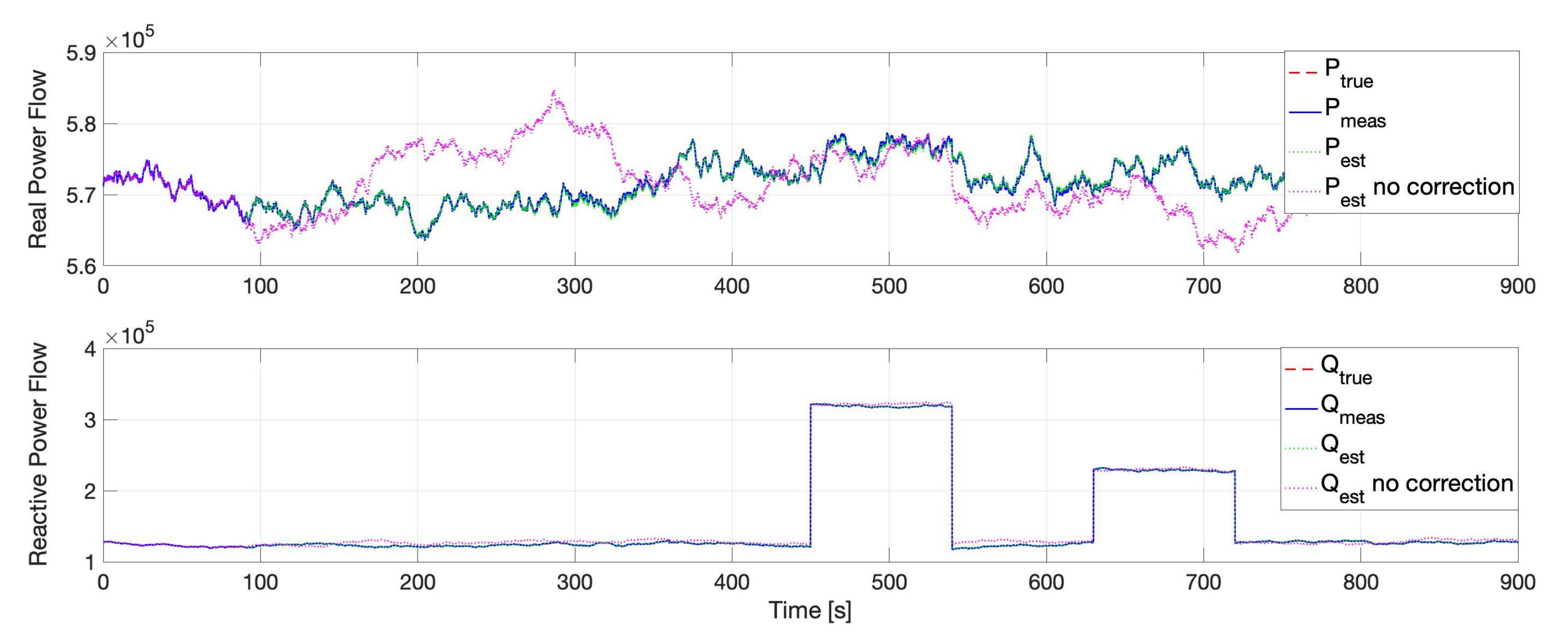
The power flows from the substation bus into the feeder, shown in Figure 8, illustrate that changes in the position of the taps created a deviation in both real and reactive power flows, while the effect of the capacitor bank connection can only be noticed clearly in the reactive power plot. The large increases in reactive power reaction at s and s and the subsequent decreases at s and s are used to correctly identify the operation of the capacitor banks. Distinguishing between the capacitor banks at bus 675 vs. bus 611 is done by comparing the information based on PMU measurements at but 671. If a large change is seen on all three phases, the capacitor bank at bus 675 has switched. If a smaller, but significant change is seen only on phase c, the capacitor bank at bus 611 has switched. Figure 8 shows the phase c power flows such that all VVC operations are shown.
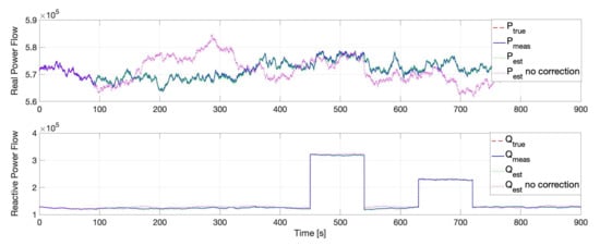
Figure 8.
Real (top) and reactive (bottom) power input to the feeder.
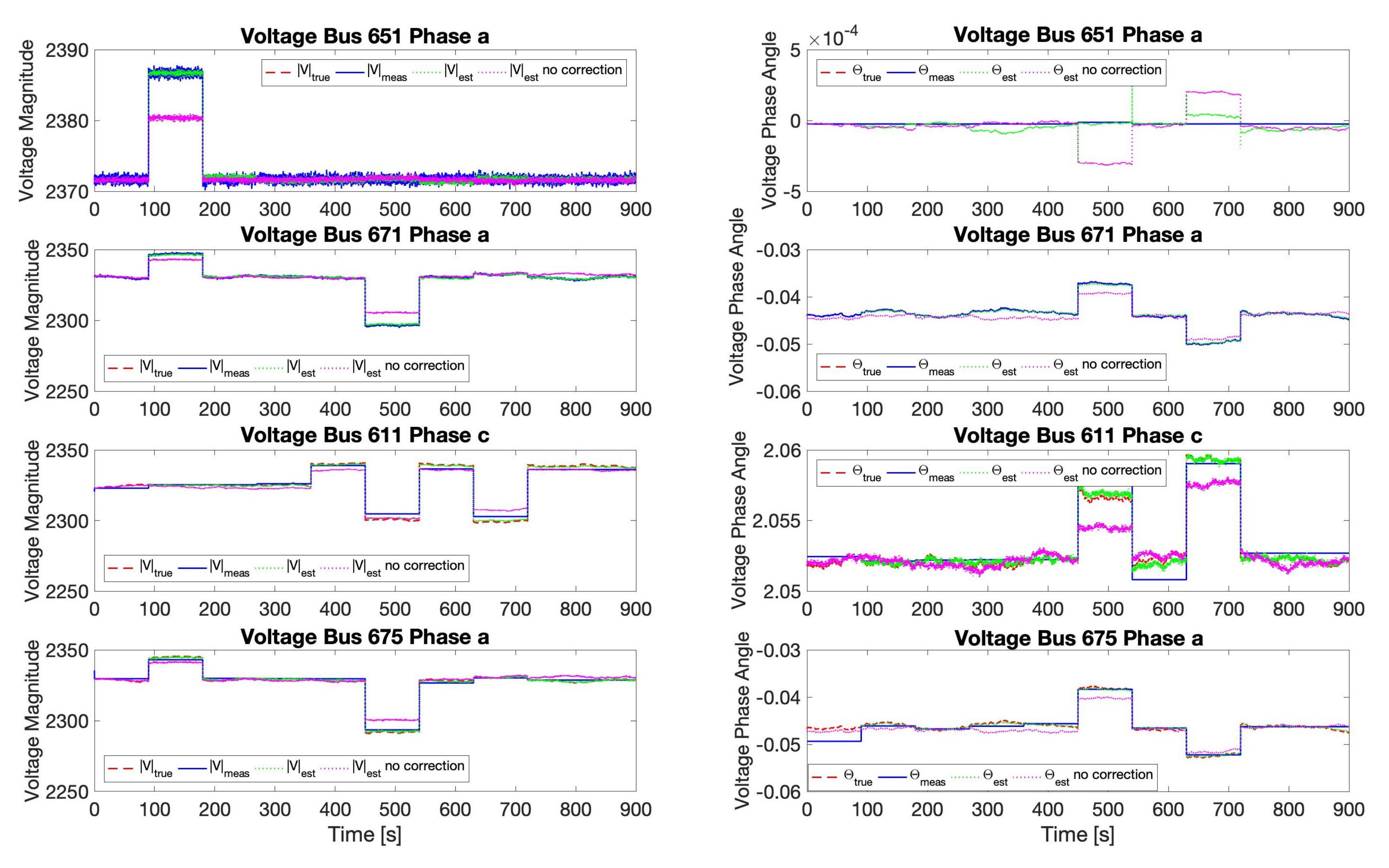
The true value, measurements and estimates of four select bus voltages are shown in Figure 9. It is clear that all of the selected bus voltages are deeply affected by the operation of VVC equipment. By observing the voltages of buses 651 and 671, it becomes very clear how that PMU measurement is useful to detect the VVC operations. Additionally, Figure 9 demonstrates that the correction applied to the measurement set after a parameter error is detected successfully brings the corrected measurement value closer to the real value of each electrical variable. In both Figure 8 and Figure 9, the magenta curves show the estimates without the correction of the parameters. These curves have major errors in the states that couple lead to incorrect operation of the system.
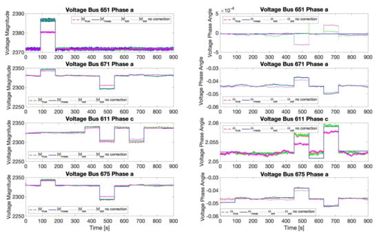
Figure 9.
Comparison of true, measured, and estimated values of bus voltages.
6. Conclusions
The presented DSSE method decouples the bad data processing of errors in measurements and parameters through the use of separate NLSE and LSE. These work together in a symbiotic relationship where the LSE ensures that the correct parameters are available and it also adds redundancy to the NLSE via SM. The scheme simplifies the job of NLSE so that it can just perform measurement error detection while the NLSE adds redundancy to the LSE via linearized measurements. NLSE is performed when a new batch of SCADA and AMI unsynchronized measurements are available, while LSE uses linearized unsynchronized measurements and PMU data. Loads are modeled as an Ornstein–Uhlenbeck stochastic process to account for the variations of the electrical variables being measured by unsynchronized measurements. A scheme to update the variance of those measurements uses the OU model to quantify the expected load dynamics into the uncertainty of SCADA and AMI linearized measurements. The VI identifies the locations on the system where SM will be most beneficial for measurement error detection in the NLSE. The results show that SM directly improved the gross error analysis tests. With these innovations working together, the proposed DSSE will use PMUs to enhance both measurement and parameter error detection on distribution grids. Considering future work, the framework extension to consider simultaneous parameter of devices gross error processing is planned.
Author Contributions
Conceptualization, R.D.T.; methodology, R.D.T.; software, R.D.T., C.R., A.R. and S.C.D.; validation, R.D.T., C.R., A.R. and S.C.D.; formal analysis, R.D.T., C.R., A.R., and S.C.D.; investigation, R.D.T., C.R., A.R. and S.C.D.; writing—review and editing, A.B. and N.G.B.; supervision, A.B. and N.G.B.; project administration, A.B.; funding acquisition, A.B. All authors have read and agreed to the published version of the manuscript.
Funding
This work was supported by NSF grant ECCS-1809739. This material is based upon work supported by the U.S. Department of Energy’s Office of Energy Efficiency and Renewable Energy (EERE) under Solar Energy Technologies Office (SETO) Agreement Number 34226.
Institutional Review Board Statement
Not applicable.
Informed Consent Statement
Not applicable.
Conflicts of Interest
The authors declare no conflict of interest.
References
- Sexauer, J.; Javanbakht, P.; Mohagheghi, S. Phasor measurement units for the distribution grid: Necessity and benefits. In Proceedings of the 2013 IEEE PES Innovative Smart Grid Technologies Conference (ISGT), Washington, DC, USA, 24–27 February 2013; pp. 1–6. [Google Scholar] [CrossRef]
- Paolone, M.; Borghetti, A.; Nucci, C.A. A synchrophasor estimation algorithm for the monitoring of active distribution networks in steady state and transient conditions. In Proceedings of the PSCC, Stockholm, Sweden, 22–26 August 2011. [Google Scholar]
- Caldarola, F.; Pantano, P.; Bilotta, E. Computation of supertrack functions for Chua’s oscillator and for Chua’s circuit with memristor. Commun. Nonlinear Sci. Numer. Simul. 2021, 94, 105568. [Google Scholar] [CrossRef]
- Abdelmalak, M.; Benidris, M.; Livani, H. A Polynomial Chaos-based Approach to Quantify Uncertainty of Solar Energy in Electric Power Distribution Systems. In Proceedings of the 2020 IEEE/PES Transmission and Distribution Conference and Exposition (T D), Chicago, IL, USA, 12–15 October 2020; pp. 1–5. [Google Scholar] [CrossRef]
- Chen, J.; Dong, Y.; Zhang, H. Distribution system state estimation: A survey of some relevant work. In Proceedings of the 35th Chinese Control Conference, Chengdu, China, 27–29 July 2016; pp. 9985–9989. [Google Scholar] [CrossRef]
- Gómez-Expósito, A.; Gómez-Quiles, C.; Džafić, I. State Estimation in Two Time Scales for Smart Distribution Systems. IEEE Trans. Smart Grid 2015, 6, 421–430. [Google Scholar] [CrossRef]
- Clements, K.A. The impact of pseudo-measurements on state estimator accuracy. In Proceedings of the IEEE PES General Meeting, Detroit, MI, USA, 24–28 July 2011; pp. 1–4. [Google Scholar] [CrossRef]
- Bretas, A.S.; Bretas, N.G.; Carvalho, B.E. Further contributions to smart grids cyber-physical security as a malicious data attack: Proof and properties of the parameter error spreading out to the measurements and a relaxed correction model. Int. J. Electr. Power Energy Syst. 2019, 104, 43–51. [Google Scholar] [CrossRef]
- Stewart, E.; Stadler, M.; Roberts, C.; Reilly, J.; Arnold, D.; Joo, J.Y. Data driven approach for monitoring, protection and control of distribution system assets using micro-PMU technology. In Proceedings of the 24th CIRED, Glasgow, Scotland, 12–15 June 2017; pp. 1–5. [Google Scholar]
- Shahsavari, A.; Farajollahi, M.; Stewart, E.; von Meier, A.; Alvarez, L.; Cortez, E.; Mohsenian-Rad, H. A data-driven analysis of capacitor bank operation at a distribution feeder using micro-PMU data. In Proceedings of the IEEE PES ISGT, Torino, Italy, 26–29 September 2017; pp. 1–5. [Google Scholar] [CrossRef]
- Alimardani, A.; Therrien, F.; Atanackovic, D.; Jatskevich, J.; Vaahedi, E. Distribution System State Estimation Based on Nonsynchronized Smart Meters. IEEE Trans. Smart Grid 2015, 6, 2919–2928. [Google Scholar] [CrossRef]
- Farajollahi, M.; Shahsavari, A.; Mohsenian-Rad, H. Tracking State Estimation in Distribution Networks Using Distribution-level Synchrophasor Data. In Proceedings of the IEEE PES General Meeting, Portland, OR, USA, 5–9 August 2018; pp. 1–5. [Google Scholar]
- Sarri, S.; Paolone, M.; Cherkaoui, R.; Borghetti, A.; Napolitano, F.; Nucci, C.A. State estimation of Active Distribution Networks: Comparison between WLS and iterated kalman-filter algorithm integrating PMUs. In Proceedings of the 2012 ISGT Europe, Berlin, Germany, 14–17 October 2012; pp. 1–8. [Google Scholar] [CrossRef]
- Huang, Z.; Schneider, K.; Nieplocha, J. Feasibility studies of applying Kalman Filter techniques to power system dynamic state estimation. In Proceedings of the IPEC, Singapore, 3–6 December 2007; pp. 376–382. [Google Scholar]
- Zhao, J.; Netto, M.; Mili, L. A Robust Iterated Extended Kalman Filter for Power System Dynamic State Estimation. IEEE Trans. Power Syst. 2017, 32, 3205–3216. [Google Scholar] [CrossRef]
- Ruben, C.; Dhulipala, S.C.; Bretas, A.S.; Guan, Y.; Bretas, N.G. Multi-objective MILP model for PMU allocation considering enhanced gross error detection: A weighted goal programming framework. Electr. Power Syst. Res. 2020, 182, 106235. [Google Scholar] [CrossRef]
- Power Standards Lab. Synchrophasors for Distribution, Microgrids: PQube 3 MicroPMU. Technical Report. Available online: http://www.jsdata.co.kr/down/MicroPMUCat.pdf (accessed on 29 September 2021).
- Wang, J.; Lu, X.; Chen, C. Guidelines for Implementing Advanced Distribution Management Systems: Requirements for DMS Integration with DERMS and Microgrids; Technical report; Argonne National Lab.: Lemont, IL, USA, 2015. [Google Scholar]
- Samarakoon, K.; Wu, J.; Ekanayake, J.; Jenkins, N. Use of delayed smart meter measurements for distribution state estimation. In Proceedings of the IEEE PES General Meeting, Detroit, MI, USA, 24–28 July 2011; pp. 1–6. [Google Scholar] [CrossRef]
- Wang, H.; Schulz, N. A load modelling algorithm for distribution system state estimation. In Proceedings of the 2001 IEEE/PES Transmission and Distribution Conference and Exposition. Developing New Perspectives (Cat. No.01CH37294), Atlanta, GA, USA, 2 November 2001; Volume 1, pp. 102–105. [Google Scholar]
- Bretas, N.G.; Piereti, S.A.; Bretas, A.S.; Martins, A.C.P. A Geometrical View for Multiple Gross Errors Detection, Identification, and Correction in Power System State Estimation. IEEE Trans. Power Syst. 2013, 28, 2128–2135. [Google Scholar] [CrossRef]
- Bretas, A.S.; Bretas, N.G.; London, J.B.; Carvalho, B.E. Cyber-Physical Power Systems State Estimation; Elsevier: Amsterdam, The Netherlands, 2021. [Google Scholar]
- Chakrabarti, S.; Kyriakides, E.; Ledwich, G.; Ghosh, A. Inclusion of PMU current phasor measurements in a power system state estimator. IET Gener. Transm. Distrib. 2010, 4, 1104–1115. [Google Scholar] [CrossRef]
- Bretas, N.G.; Bretas, A.S.; Piereti, S.A. Innovation concept for measurement gross error detection and identification in power system state estimation. IET Gener. Transm. Distrib. 2011, 5, 603–608. [Google Scholar] [CrossRef]
- Bretas, N.G.; Bretas, A.S.; Martins, A.C.P. Convergence Property of the Measurement Gross Error Correction in Power System State Estimation, Using Geometrical Background. IEEE Trans. Power Syst. 2013, 28, 3729–3736. [Google Scholar] [CrossRef]
- Bretas, A.; Bretas, N.; Braunstein, S.; Rossoni, A.; Trevizan, R. Multiple gross errors detection, identification and correction in three-phase distribution systems WLS state estimation: A per-phase measurement error approach. Electr. Power Syst. Res. 2017, 151, 174–185. [Google Scholar] [CrossRef]
- Lu, C.N.; Teng, J.H.; Liu, W.E. Distribution system state estimation. IEEE Trans. Power Syst. 1995, 10, 229–240. [Google Scholar] [CrossRef]
- Baran, M.E.; Kelley, A.W. A branch-current-based state estimation method for distribution systems. IEEE Trans. Power Syst. 1995, 10, 483–491. [Google Scholar] [CrossRef]
- Perninge, M.; Knazkins, V.; Amelin, M.; Soder, L. Risk Estimation of Critical Time to Voltage Instability Induced by Saddle-Node Bifurcation. IEEE Trans. Power Syst. 2010, 25, 1600–1610. [Google Scholar] [CrossRef]
- Roberts, C.; Stewart, E.M.; Milano, F. Validation of the Ornstein-Uhlenbeck process for load modeling based on μPMU measurements. In Proceedings of the PSCC, Genoa, Italy, 20–24 June 2016; pp. 1–7. [Google Scholar] [CrossRef]
- Arató, M.; Baran, S.; Ispány, M. Functionals of complex Ornstein-Uhlenbeck processes. Comput. Math. Appl. 1999, 37, 1–13. [Google Scholar] [CrossRef][Green Version]
- Bibbona, E.; Panfilo, G.; Tavella, P. The Ornstein-Uhlenbeck process as a model of a low pass filtered white noise. Metrologia 2008, 45, S117. [Google Scholar] [CrossRef]
- Wooding, R.A. The Multivariate Distribution of Complex Normal Variables. Biometrika 1956, 43, 212–215. [Google Scholar] [CrossRef]
- Bretas, A.S.; Rossoni, A.; Trevizan, R.D.; Bretas, N.G. Distribution networks nontechnical power loss estimation: A hybrid data-driven physics model-based framework. Electr. Power Syst. Res. 2020, 186, 106397. [Google Scholar] [CrossRef]
- Dhulipala, S.C.; Ruben, C.; Bretas, A.; Bretas, N. Improvement in Vulnerability and Error Analysis: A Synthetic Measurement Approach. In Proceedings of the 2019 IEEE Power Energy Society General Meeting, Atlanta, GA, USA, 4–8 August 2019; pp. 1–5. [Google Scholar]
- Kersting, W.H. Distribution System Modeling and Analysis; CRC Press: Boca Raton, FL, USA, 2006. [Google Scholar]
Publisher’s Note: MDPI stays neutral with regard to jurisdictional claims in published maps and institutional affiliations. |
© 2021 by the authors. Licensee MDPI, Basel, Switzerland. This article is an open access article distributed under the terms and conditions of the Creative Commons Attribution (CC BY) license (https://creativecommons.org/licenses/by/4.0/).

