
Assessment of Heavy Metal Contamination and Ecological Risk in Urban River Sediments: A Case Study from Leyte, Philippines

 ,
,  ,
,
Abstract

1. Introduction
2. Materials and Methods
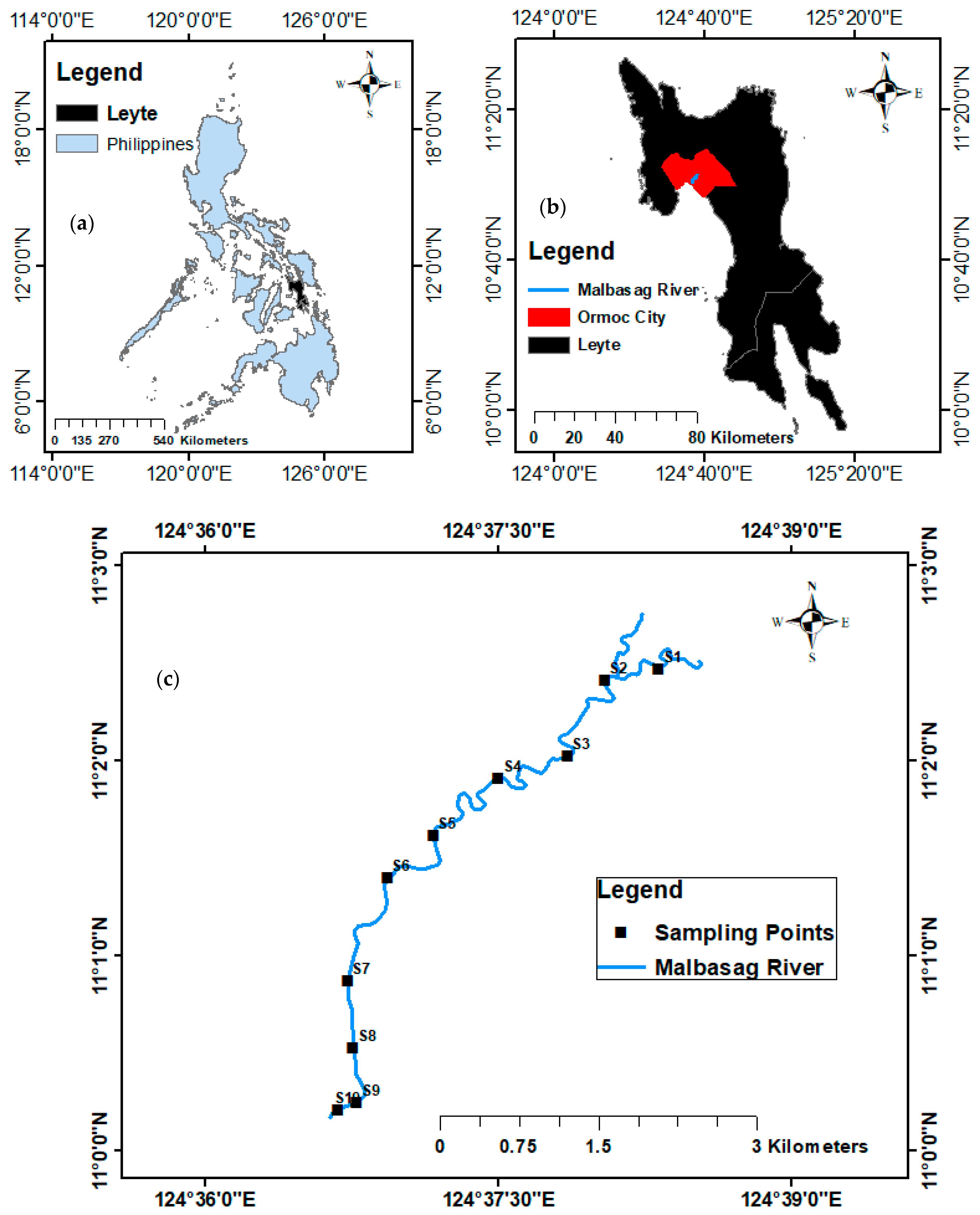
2.1. Study Area
2.2. Sampling Sites
2.3. Sample Collection
2.4. Chemical Analysis
2.4.1. Reagents and Standards
2.4.2. Analysis of Sediment Samples
2.5. Analytical Process for Physicochemical Parameter
2.6. Quality Control
2.7. Sediment Quality Guidelines
2.8. Pollution Assessment
2.8.1. Contamination Factor (CF)
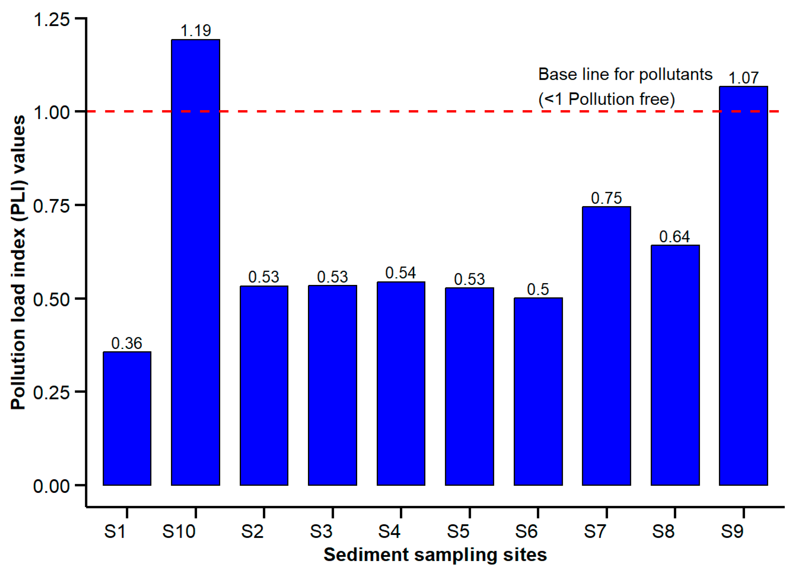
2.8.2. Pollution Load Index (PLI)
2.8.3. Geo-Accumulation Index (Igeo)
2.8.4. Enrichment Factor (EF)
2.9. Potential Ecological Risk Index (RI)
2.10. Toxic Units
2.11. Toxic Risk Index (TRI)
2.12. Modified Hazard Quotient (mHQ)
2.13. Statistical Analyses
3. Results and Discussion
3.1. The Physicochemical Properties of Sediment Samples in the Study Area
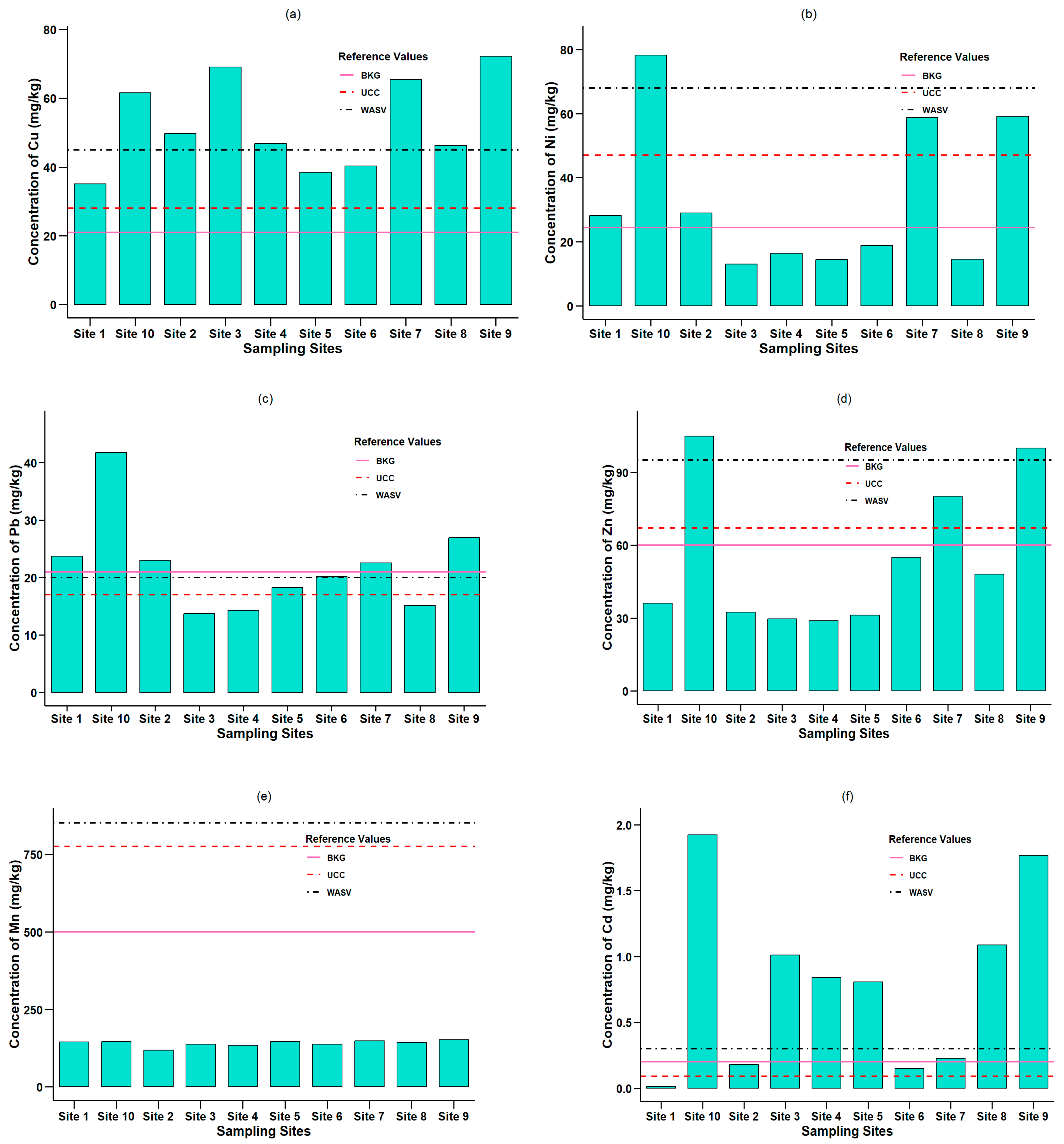
3.2. Heavy Metal Concentration
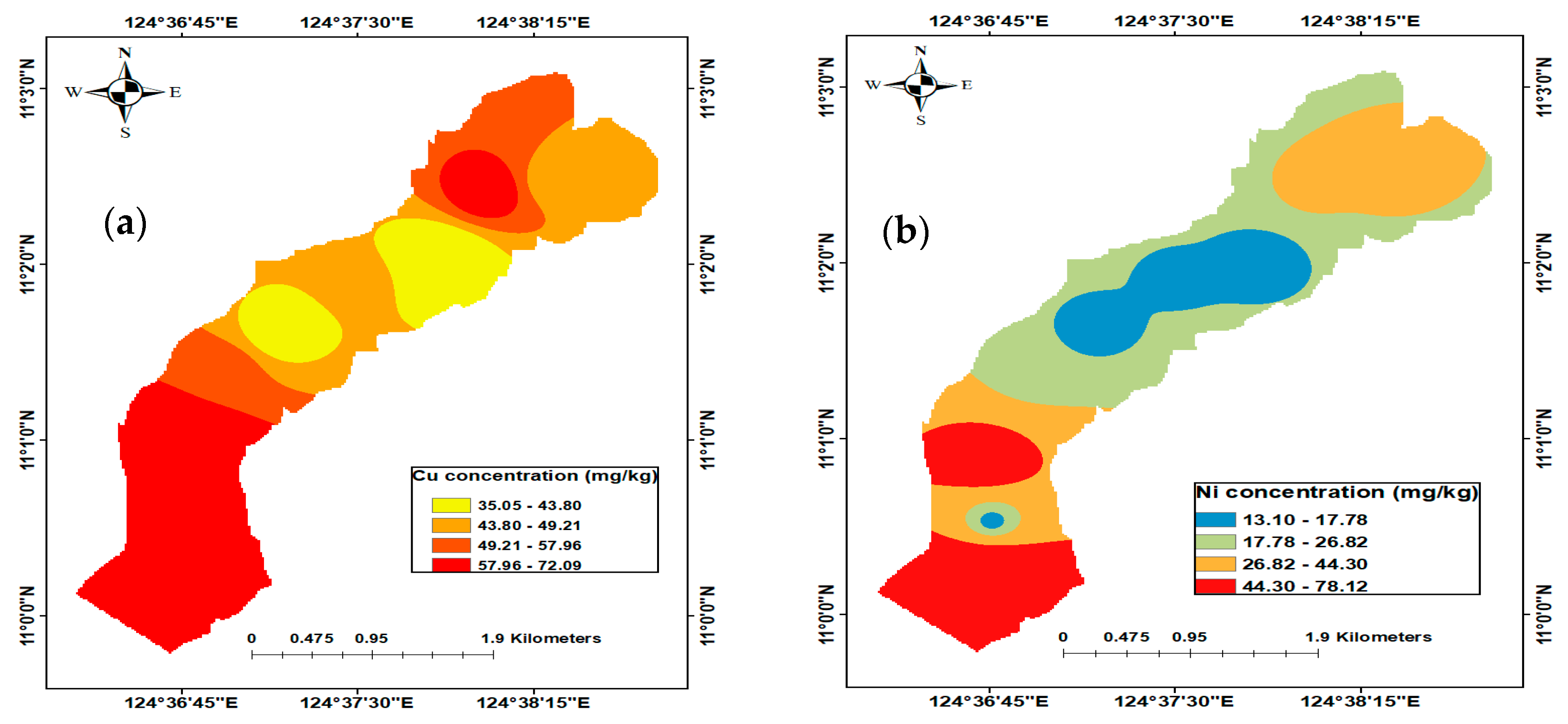
3.2.1. Copper (Cu)
3.2.2. Nickel (Ni)
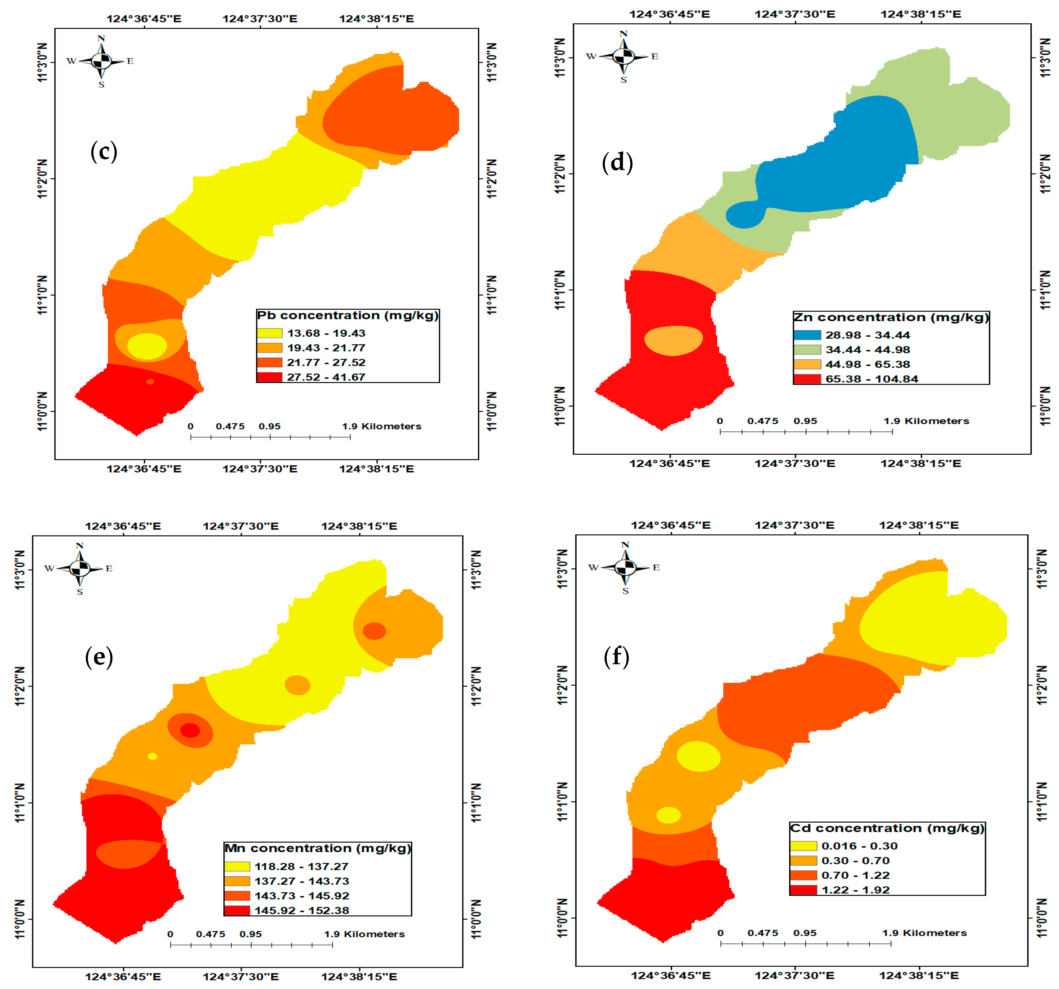
3.2.3. Lead (Pb)
3.2.4. Zinc (Zn)
3.2.5. Manganese (Mn)
3.2.6. Cadmium (Cd)
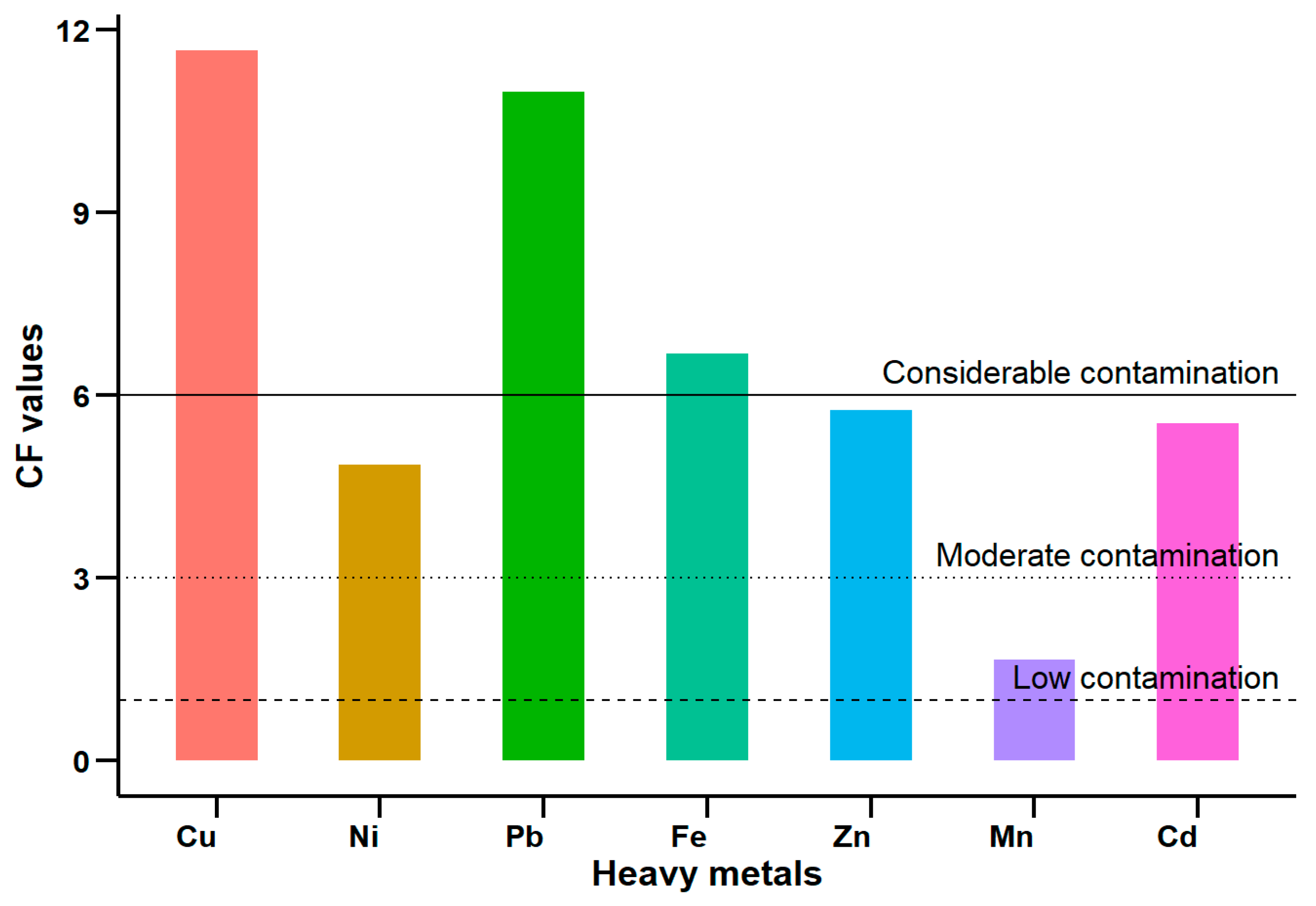
3.3. Geochemical Indicators of Contaminated Sediments
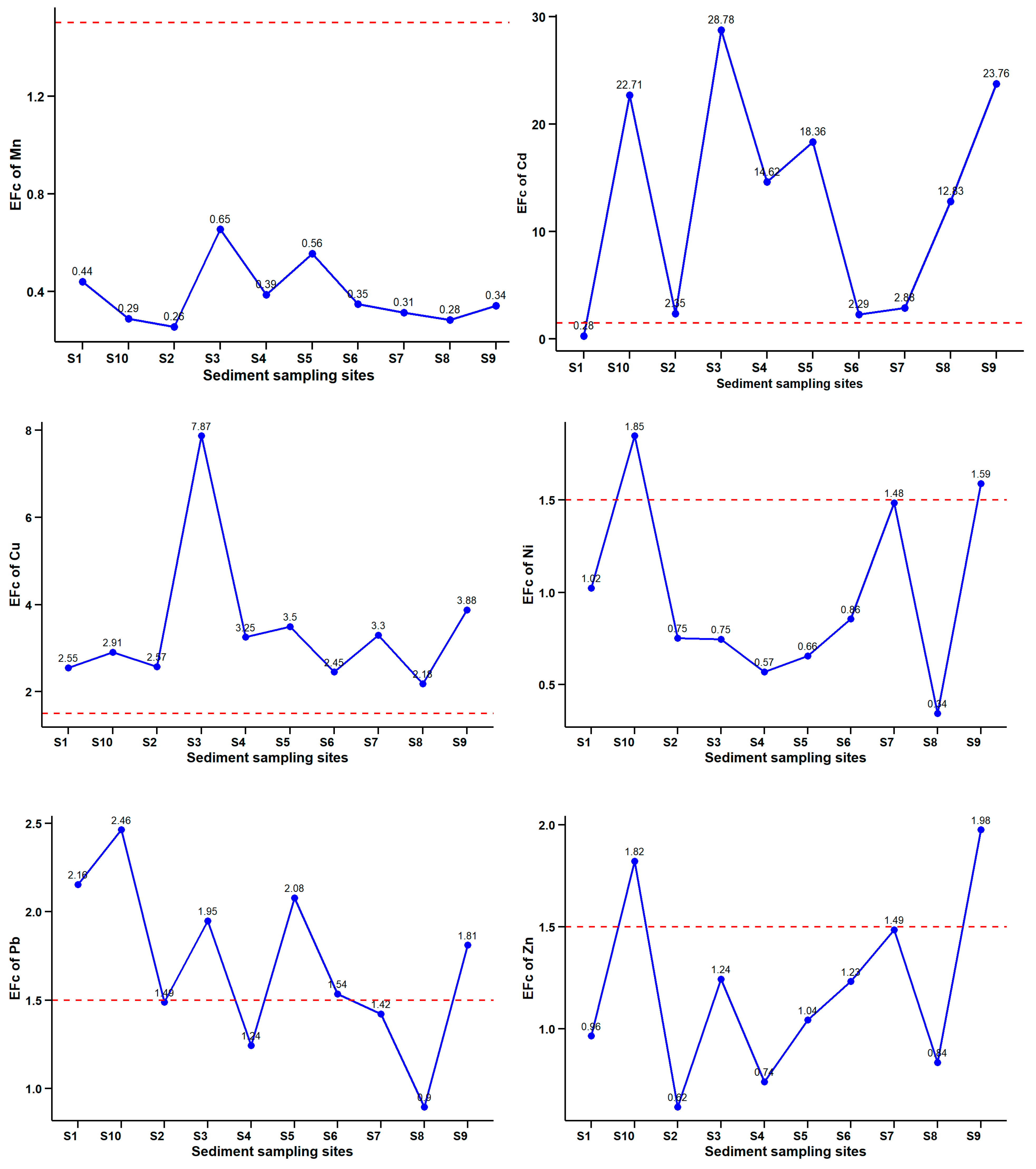
Contamination Factor (CF), Pollution Load Index (PLI), Geo-Accumulation Index (Igeo), and Enrichment Factor (EF)
3.4. Ecological Risk
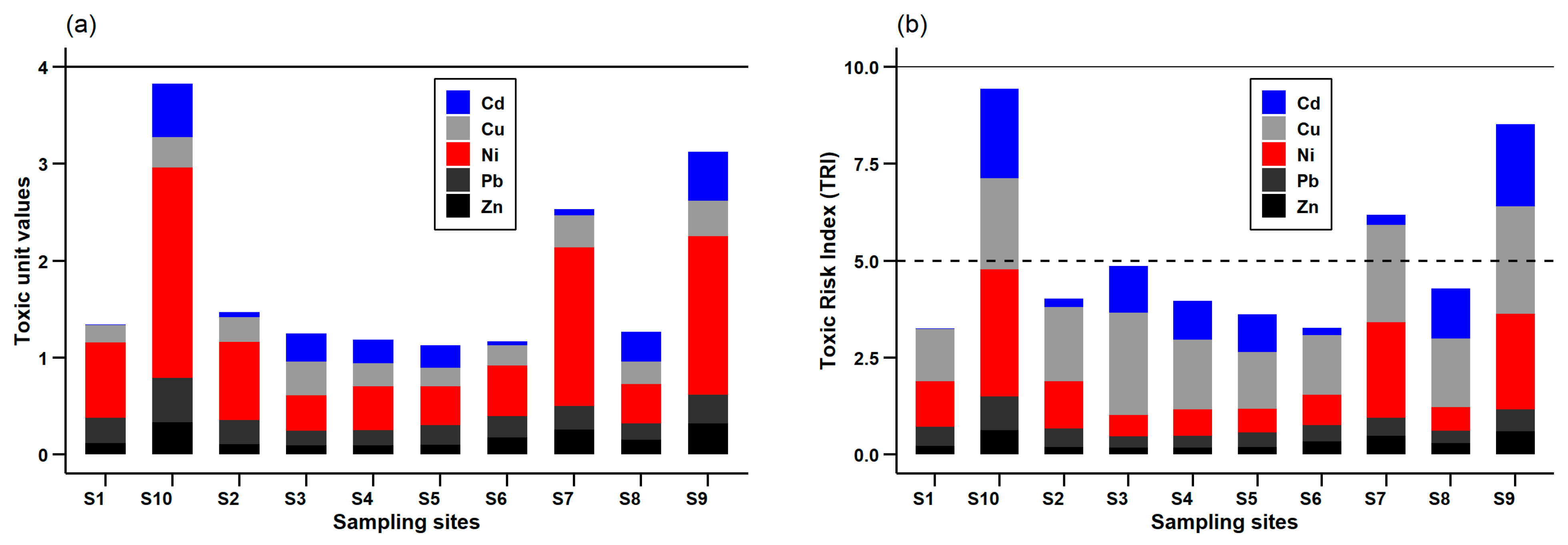
3.5. Assessment of Heavy Metal Contamination by Using Toxic Unit (TU) and Toxic Risk Index (TRI)
3.6. Sediment Hazard Quotient Evaluation
3.7. Sources of Heave Metal in the Study Area
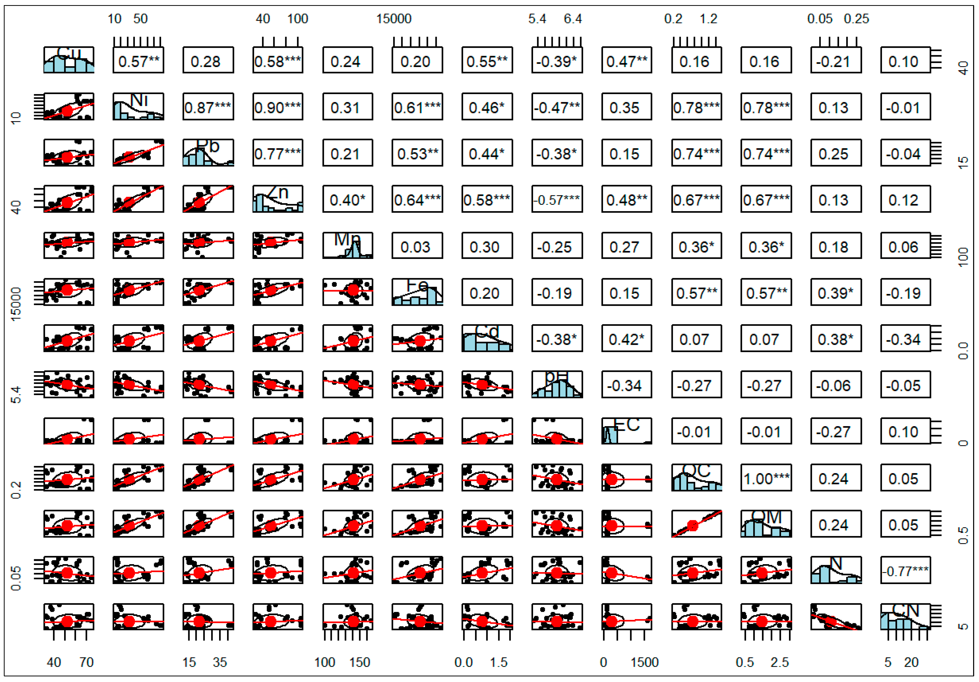
3.7.1. Correlation Coefficient Analysis (CCA)
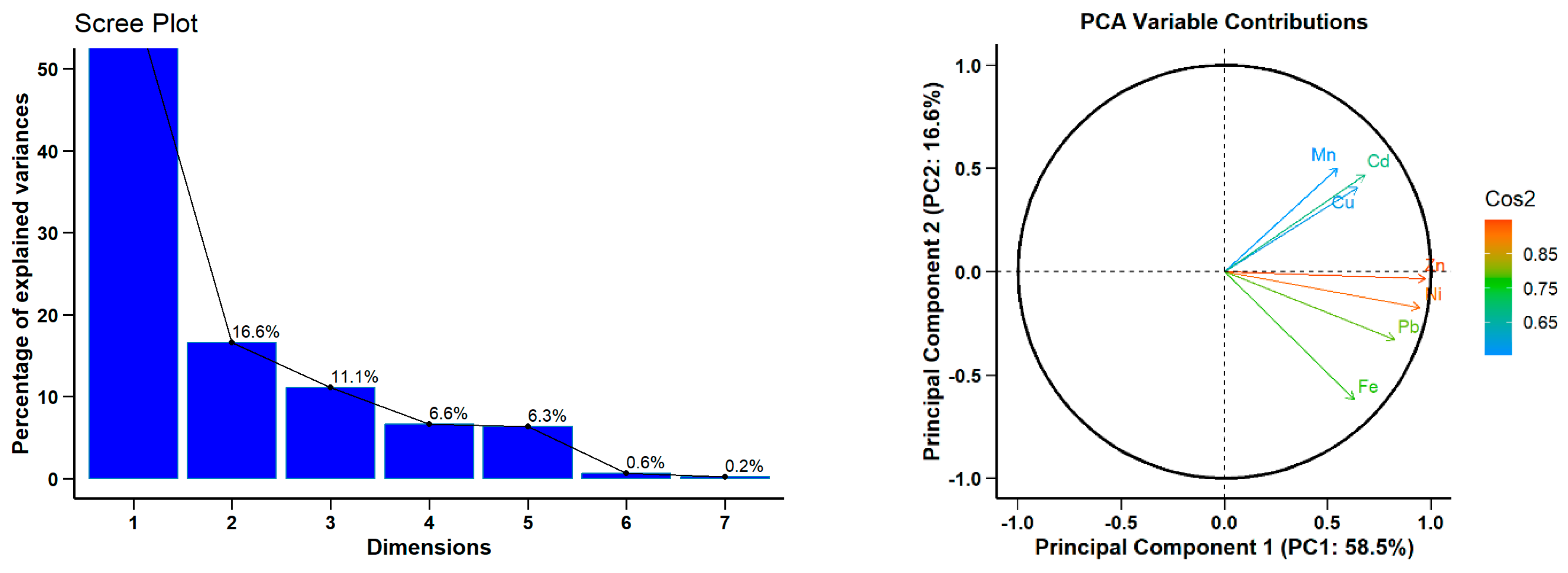
3.7.2. Principal Component Analysis (PCA)
3.8. Spatial Distribution
3.9. Limitations of the Study
4. Conclusions
Supplementary Materials
Author Contributions
Funding
Data Availability Statement
Acknowledgments
Conflicts of Interest
References
- Gopal, V.; Krishnamurthy, R.R.; Vignesh, R.; Nathan, C.S.; Anshu, R.; Kalaivanan, R.; Mohana, P.; Magesh, N.S.; Bharath, K.M.; Bessa, A.Z.E.; et al. Assessment of heavy metal contamination in the surface sediments of the Vedaranyam coast, Southern India. Reg. Stud. Mar. Sci. 2023, 65, 103081. [Google Scholar] [CrossRef]
- Siddique MA, M.; Rahman, M.; Rahman SM, A.; Hassan, M.R.; Fardous, Z.; Chowdhury MA, Z.; Hossain, M.B. Assessment of heavy metal contamination in the surficial sediments from the lower Meghna River estuary, Noakhali coast, Bangladesh. Int. J. Sediment Res. 2021, 36, 384–391. [Google Scholar] [CrossRef]
- Ke, X.; Gui, S.; Huang, H.; Zhang, H.; Wang, C.; Guo, W. Ecological risk assessment and source identification for heavy metals in surface sediment from the Liaohe River protected area, China. Chemosphere 2017, 175, 473–481. [Google Scholar] [CrossRef] [PubMed]
- Usman, Q.A.; Muhammad, S.; Ali, W.; Yousaf, S.; Jadoon, I.A. Spatial distribution and provenance of heavy metal contamination in the sediments of the Indus River and its tributaries, North Pakistan: Evaluation of pollution and potential risks. Environ. Technol. Innov. 2021, 21, 101184. [Google Scholar] [CrossRef]
- Xu, Y.Y.; Liu, Y.C.; Zhang, J.; Chen, M.; Liu, Z.F.; Li, R.X.; Qiaolipanguli, T. Spatial distribution and risk assessment of nitrogen and heavy metals in typical watershed of the upper reaches of Ganjiang River. Earth Environ. 2020, 48, 574–583. [Google Scholar]
- Dey, M.; Akter, A.; Islam, S.; Dey, S.C.; Choudhury, T.R.; Fatema, K.J.; Begum, B.A. Assessment of contamination level, pollution risk and source apportionment of heavy metals in the Halda River water, Bangladesh. Heliyon 2021, 7, e08625. [Google Scholar] [CrossRef] [PubMed]
- Yüksel, B.; Ustaoğlu, F.; Yazman, M.M.; Şeker, M.E.; Öncü, T. Exposure to potentially toxic elements through ingestion of canned non-alcoholic drinks sold in Istanbul, Türkiye: A health risk assessment study. J. Food Compos. Anal. 2023, 121, 105361. [Google Scholar] [CrossRef]
- Wang, Z.; Lin, K.; Liu, X. Distribution and pollution risk assessment of heavy metals in the surface sediment of the intertidal zones of the Yellow River Estuary, China. Mar. Pollut. Bull. 2022, 174, 113286. [Google Scholar] [CrossRef]
- Xie, Q.; Ren, B. Pollution and risk assessment of heavy metals in rivers in the antimony capital of Xikuangshan. Sci. Rep. 2022, 12, 14393. [Google Scholar] [CrossRef]
- Aziz KH, H.; Mustafa, F.S.; Omer, K.M.; Hama, S.; Hamarawf, R.F.; Rahman, K.O. Heavy metal pollution in the aquatic environment: Efficient and low-cost removal approaches to eliminate their toxicity: A review. RSC Adv. 2023, 13, 17595–17610. [Google Scholar] [CrossRef]
- Xu, Y.; Liao, X.; Guo, B. Assessment of Heavy Metal Pollution in Water Sediment and Study on Pollution Mechanism—Taking the Weihe River Basin in China as an Example. Processes 2023, 11, 416. [Google Scholar] [CrossRef]
- Debnath, A.; Singh, P.K.; Sharma, Y.C. Metallic contamination of global river sediments and latest developments for their remediation. J. Environ. Manag. 2021, 298, 113378. [Google Scholar] [CrossRef]
- Hamil, S.; Baha, M.; Arab, S.; Doukhandji, N.; Arab, A. A Multivariate Analysis of Water Quality in Lake Ghrib, Algeria. In Recent Advances in Environmental Science from the Euro-Mediterranean and Surrounding Regions, Proceedings of the Euro-Mediterranean Conference for Environmental Integration (EMCEI-1), Sousse, Tunisia, 20–25 November 2017; Springer International Publishing: Berlin/Heidelberg, Germany, 2018; pp. 805–807. [Google Scholar]
- El-Alfy, M.A.; El-Amier, Y.A.; El-Eraky, T.E. Land use/cover and eco-toxicity indices for identifying metal contamination in sediments of drains, Manzala Lake, Egypt. Heliyon 2020, 6, e03177. [Google Scholar] [CrossRef] [PubMed]
- Bessa, A.Z.E.; Ngueutchoua, G.; Janpou, A.K.; El-Amier, Y.A.; Nguetnga, O.-A.N.N.M.; Kayou, U.R.K.; Bisse, S.B.; Mapuna, E.C.N.; Armstrong-Altrin, J.S. Heavy metal contamination and its ecological risks in the beach sediments along the Atlantic Ocean (Limbe coastal fringes, Cameroon). Earth Syst. Environ. 2021, 5, 433–444. [Google Scholar] [CrossRef]
- Avkopashvili, M.; Avkopashvili, G.; Avkopashvili, I.; Asanidze, L.; Matchavariani, L.; Gongadze, A.; Gakhokidze, R. Mining-related metal pollution and ecological risk factors in South-Eastern Georgia. Sustainability 2022, 14, 5621. [Google Scholar] [CrossRef]
- Bux, R.K.; Haider, S.I.; Batool, M.; Solangi, A.R.; Shah, Z.; Karimi-Maleh, H.; Sen, F. Assessment of heavy metal contamination and its sources in urban soils of district Hyderabad, Pakistan using GIS and multivariate analysis. Int. J. Environ. Sci. Technol. 2021, 19, 7901–7913. [Google Scholar] [CrossRef]
- Khan, M.; Omer, T.; Ellahi, A.; Ur Rahman, Z.; Niaz, R.; Ahmad Lone, S. Monitoring and assessment of heavy metal contamination in surface water of selected rivers. Geocarto Int. 2023, 38, 2256313. [Google Scholar] [CrossRef]
- Ali, M.M.; Ali, M.L.; Islam, M.S.; Rahman, M.Z. Preliminary assessment of heavy metals in water and sediment of Karnaphuli River, Bangladesh. Environ. Nanotechnol. Monit. Manag. 2016, 5, 27–35. [Google Scholar] [CrossRef]
- Islam, M.S.; Hossain, M.B.; Matin, A.; Sarker MS, I. Assessment of heavy metal pollution, distribution and source apportionment in the sediment from Feni River estuary, Bangladesh. Chemosphere 2018, 202, 25–32. [Google Scholar] [CrossRef]
- Rahman, M.S.; Hossain, M.B.; Babu, S.O.F.; Ahmed, A.S.; Jolly, Y.; Choudhury, T.; Begum, B.; Kabir, J.; Akter, S. Source of metal contamination in sediment, their ecological risk, and phytoremediation ability of the studied mangrove plants in ship breaking area, Bangladesh. Mar. Pollut. Bull. 2019, 141, 137–146. [Google Scholar] [CrossRef]
- Maanan, M.; Saddik, M.; Maanan, M.; Chaibi, M.; Assobhei, O.; Zourarah, B. Environmental and ecological risk assessment of heavy metals in sediments of Nador lagoon, Morocco. Ecol. Indic. 2015, 48, 616–626. [Google Scholar] [CrossRef]
- Topaldemir, H.; Taş, B.; Yüksel, B.; Ustaoğlu, F. Potentially hazardous elements in sediments and Ceratophyllum demersum: An ecotoxicological risk assessment in Miliç Wetland, Samsun, Türkiye. Environ. Sci. Pollut. Res. 2023, 30, 26397–26416. [Google Scholar] [CrossRef]
- Zhang, Z.; Lu, Y.; Li, H.; Tu, Y.; Liu, B.; Yang, Z. Assessment of heavy metal contamination, distribution and source identification in the sediments from the Zijiang River, China. Sci. Total Environ. 2018, 645, 235–243. [Google Scholar] [CrossRef] [PubMed]
- Zhang, Y.; Zhang, H.; Zhang, Z.; Liu, C.; Sun, C.; Zhang, W.; Marhaba, T. pH effect on heavy metal release from a polluted sediment. J. Chem. 2018, 2018, 7597640. [Google Scholar] [CrossRef]
- Birch, G.F. Determination of sediment metal background concentrations and enrichment in marine environments–a critical review. Sci. Total Environ. 2017, 580, 813–831. [Google Scholar] [CrossRef]
- UNCTAD. Review of Maritime Transport; UNCTAD/RMT: New York, NY, USA, 2015. [Google Scholar]
- Sankhla, M.S.; Kumar, R.; Biswas, A. Dynamic nature of heavy metal toxicity in water and sediments of Ayad River with climatic change. Int. J. Hydrol. 2019, 3, 339–343. [Google Scholar] [CrossRef]
- Abdel-Ghani, N.T.; Elchaghaby, G.A. Influence of operating conditions on the removal of Cu, Zn, Cd and Pb ions from wastewater by adsorption. Int. J. Environ. Sci. Technol. 2007, 4, 451–456. [Google Scholar] [CrossRef]
- Nouri, J.; Lorestani, B.; Yousefi, N.; Khorasani, N.; Hasani, A.H.; Seif, F.; Cheraghi, M. Phytoremediation potential of native plants grown in the vicinity of Ahangaran lead–zinc mine (Hamedan, Iran). Environ. Earth Sci. 2011, 62, 639–644. [Google Scholar] [CrossRef]
- Pearson, M.L.; Oliver, J.G. Reconnaissance Report: Flooding Resulting from Typhoon Uring in Ormoc City, Leyte Province, the Philippines; Geotechnical Laboratory: Monrovia, CA, USA, 1992. [Google Scholar]
- Zhang, Z.; Wang, J.J.; Ali, A.; DeLaune, R.D. Heavy metals and metalloid contamination in Louisiana Lake Pontchartrain Estuary along I-10 Bridge. Transp. Res. Part D Transp. Environ. 2016, 44, 66–77. [Google Scholar] [CrossRef]
- Tabios, G.Q., III. Water Resources Systems of the Philippines: Modeling Studies; Springer Nature: Berlin/Heidelberg, Germany, 2020; Volume 4. [Google Scholar]
- WWF & BPI. Business Risk Assessment and the Management of Climate Change Impacts. 2013. Available online: https://environmentalmigration.iom.int/sites/g/files/tmzbdl1411/files/documents/2023-10/business-risk-assessment-and-the-management-of-climate-change-impacts-12-cities.pdf (accessed on 21 October 2024).
- Climate-Data.org. Available online: https://en.climate-data.org/asia/philippines/leyte/ormoc-3489/t/july-7/ (accessed on 23 October 2024).
- Islam, M.S.; Ahmed, M.K.; Raknuzzaman, M.; Habibullah-Al-Mamun, M.; Islam, M.K. Heavy metal pollution in surface water and sediment: A preliminary assessment of an urban river in a developing country. Ecol. Indic. 2015, 48, 282–291. [Google Scholar] [CrossRef]
- USEPA. Method 3050B: Acid Digestion of Sediments, Sludges, and Soils; USEPA: Washington, DC, USA, 1996.
- Nelson, D.W.; Sommers, L.E. Total carbon, organic carbon, and organic matter. Methods Soil Anal. Part 3 Chem. Methods 1996, 5, 961–1010. [Google Scholar]
- Glazovskaya, M.A. Methodological Guidelines for Forecasting the Geochemical Susceptibility of Soils to Technogenic Pollution (Draft); Working Paper and Preprint 91/1; ISRIC: Wageningen, The Netherlands, 1991; p. 43. [Google Scholar]
- Rahman, M.S.; Ahmed, Z.; Seefat, S.M.; Alam, R.; Islam, A.R.M.T.; Choudhury, T.R.; Begum, B.A.; Idris, A.M. Assessment of heavy metal contamination in sediment at the newly established tannery industrial Estate in Bangladesh: A case study. Environ. Chem. Ecotoxicol. 2022, 4, 1–12. [Google Scholar] [CrossRef]
- Bode, P. Instrumental and Organizational Aspects of a Neutron Activation Analysis Laboratory. Doctor’s Thesis, Technische Universiteit Delft, Delft, The Netherlands, 1998. [Google Scholar]
- Rahman, M.S.; Saha, N.; Molla, A.H. Potential ecological risk assessment of heavy metal contamination in sediment and water body around Dhaka export processing zone, Bangladesh. Environ. Earth Sci. 2014, 71, 2293–2308. [Google Scholar] [CrossRef]
- MacDonald, D.D.; Ingersoll, C.G.; Berger, T.A. Development and evaluation of consensus-based sediment quality guidelines for freshwater ecosystems. Arch. Environ. Contam. Toxicol. 2000, 39, 20–31. [Google Scholar] [CrossRef]
- Xu, Z.Q.; Ni, S.J.; Tuo, X.G.; Zhang, C.J. Calculation of heavy metals’ toxicity coefficient in the evaluation of potential ecological risk index. Environ. Sci Technol 2008, 31, 112–115. [Google Scholar]
- Mazurek, R.; Kowalska, J.; Gąsiorek, M.; Zadrożny, P.; Józefowska, A.; Zaleski, T.; Kępka, W.; Tymczuk, M.; Orłowska, K. Assessment of heavy metals contamination in surface layers of Roztocze National Park Forest soils (SE Poland) by indices of pollution. Chemosphere 2017, 168, 839–850. [Google Scholar] [CrossRef]
- Covelli, S.T.E.F.A.N.O.; Fontolan, G. Application of a normalization procedure in determining regional geochemical baselines: Gulf of Trieste, Italy. Environ. Geol. 1997, 30, 34–45. [Google Scholar] [CrossRef]
- Rubio, B.; Nombela, M.; Vilas, F. Geochemistry of major and trace elements in sediments of the Ria de Vigo (NW Spain): An assessment of metal pollution. Mar. Pollut. Bull. 2000, 40, 968–980. [Google Scholar] [CrossRef]
- Sakan, S.M.; Đorđević, D.S.; Manojlović, D.D.; Predrag, P.S. Assessment of heavy metal pollutants accumulation in the Tisza River sediments. J. Environ. Manag. 2009, 90, 3382–3390. [Google Scholar] [CrossRef]
- Hakanson, L. An ecological risk index for aquatic pollution control. A sedimentological approach. Water Res. 1980, 14, 975–1001. [Google Scholar] [CrossRef]
- Turekian, K.K.; Wedepohl, K.H. Distribution of the elements in some major units of the earth’s crust. Geol. Soc. Am. Bull. 1961, 72, 175–192. [Google Scholar] [CrossRef]
- Tomlinson, D.L.; Wilson, J.G.; Harris, C.R.; Jeffrey, D.W. Problems in the assessment of heavy-metal levels in estuaries and the formation of a pollution index. Helgoländer Meeresunters. 1980, 33, 566–575. [Google Scholar] [CrossRef]
- Muller, G. Index of Geoaccumulation in Sediments of the Rhine River. Geo J. 1969, 2, 108–118. [Google Scholar]
- Bhuiyan, M.A.; Parvez, L.; Islam, M.A.; Dampare, S.B.; Suzuki, S. Heavy metal pollution of coal mine-affected agricultural soils in the northern part of Bangladesh. J. Hazard. Mater. 2010, 173, 384–392. [Google Scholar] [CrossRef]
- Mason, B.J. Introduction to Geochemistry, 3rd ed.; John Wiley: New York, NY, USA, 1966. [Google Scholar]
- Atgin, R.S.; El-Agha, O.; Zararsız, A.; Kocataş, A.; Parlak, H.; Tuncel, G. Investigation of the sediment pollution in Izmir Bay: Trace elements. Spectrochim. Acta Part B 2000, 55, 1151–1164. [Google Scholar] [CrossRef]
- Hu, J.; Lin, B.; Yuan, M.; Lao, Z.; Wu, K.; Zeng, Y.; Liang, Z.; Li, H.; Li, Y.; Zhu, D.; et al. Trace metal pollution and ecological risk assessment in agricultural soil in Dexing Pb/Zn mining area, China. Environ. Geochem. Health 2018, 41, 967–980. [Google Scholar] [CrossRef]
- Taylor, S.R.; McLennan, S.M. The Continental Crust: Its Composition and Evolution; Blackwell Scientific: Hoboken, NJ, USA, 1985. [Google Scholar]
- Bai, J.; Xiao, R.; Cui, B.; Zhang, K.; Wang, Q.; Liu, X.; Gao, H.; Huang, L. Assessment of heavy metal pollution in wetland soils from the young and old reclaimed regions in the Pearl River Estuary, South China. Environ. Pollut. 2011, 159, 817–824. [Google Scholar] [CrossRef]
- Pedersen, F.; Bjørnestad, E.; Andersen, H.V.; Kjølholt, J.; Poll, C. Characterization of sediments from Copenhagen Harbour by use of biotests. Water Sci. Technol. 1998, 37, 233–240. [Google Scholar] [CrossRef]
- Zhang, G.; Bai, J.; Xiao, R.; Zhao, Q.; Jia, J.; Cui, B.; Liu, X. Heavy metal fractions and ecological risk assessment in sediments from urban, rural and reclamation-affected rivers of the Pearl River Estuary, China. Chemosphere 2017, 184, 278–288. [Google Scholar] [CrossRef]
- Persaud, D.J.R.H.A.; Jaagumagi, R.; Hayton, A. Guidelines for the Protection and Management of Aquatic Sediment Quality in Ontario; Ontario Ministry of the Environment: Toronto, ON, Canada, 1993. [Google Scholar]
- Long, E.R.; Macdonald, D.D.; Smith, S.L.; Calder, F.D. Incidence of adverse biological effects within ranges of chemical concentrations in marine and estuarine sediments. Environ. Manag. 1995, 19, 81–97. [Google Scholar] [CrossRef]
- US EPA (US Environmental Protection Agency). Screening Level Ecological Risk Assessment Protocol for Hazardous Waste Combustion Facilities, Appendix E: Toxicity Reference Values; US Environmental Protection Agency: Washington, DC, USA, 1999; Volume 3, EPA 530-D99-001C.
- Benson, N.U.; Adedapo, A.E.; Fred-Ahmadu, O.H.; Williams, A.B.; Udosen, E.D.; Ayejuyo, O.O.; Olajire, A.A. New ecological risk indices for evaluating heavy metals contamination in aquatic sediment: A case study of the Gulf of Guinea. Reg. Stud. Mar. Sci. 2018, 18, 44–56. [Google Scholar] [CrossRef]
- Costa, C.N.; Castilhos, D.D.; Castilhos RM, V.; Konrad, E.E.; Passianoto, C.C.; Rodrigues, C.G. Tannery sludge effects on soil chemical properties, matter yield and nutrients uptake by soybean. Rev. Bras. Agrociência 2001, 7, 189–191. [Google Scholar]
- Wang, X.S.; Qin, Y. Spatial distribution of metals in urban topsoils of Xuzhou (China): Controlling factors and environmental implications. Environ. Geol. 2006, 49, 905–914. [Google Scholar] [CrossRef]
- Rudnick, R.L.; Gao, S. Composition of the Continental Crust. In Treatise on Geochemistry, Holland, H.D., Turekian, K.K., Eds.; Elsevier: Amsterdam, The Netherlands, 2003; Volume 3, pp. 1–64. [Google Scholar]
- CNEMC—China National Environmental Monitoring Center. The Background Values of Elements in Chinese Soils; Environmental Science Press of China: Beijing, China, 1990; pp. 330–493. [Google Scholar]
- United Nations Environment Programme (UNEP) and World Health Organization (WHO). Global Environment Monitoring System (GEMS)—Background Concentrations of Trace Metals in Soils; UNEP: Nairobi, Kenya, 1992. [Google Scholar]
- Zhang, J.E.; Liu, J.L.; Ouyang, Y.; Liao, B.W.; Zhao, B.L. Removal of nutrients and heavy metals from wastewater with mangrove Sonneratia apetala Buch-Ham. Ecol. Eng. 2010, 36, 807–812. [Google Scholar] [CrossRef]
- Suthar, S.; Nema, A.K.; Chabukdhara, M.; Gupta, S.K. Assessment of metals in water and sediments of Hindon River, India: Impact of industrial and urban discharges. J. Hazard. Mater. 2009, 171, 1088–1095. [Google Scholar] [CrossRef]
- Pacle Decena, S.C.; Sanita Arguelles, M.; Liporada Robel, L. Assessing heavy metal contamination in surface sediments in an urban river in the Philippines. Pol. J. Environ. Stud. 2018, 27, 1983–1995. [Google Scholar] [CrossRef] [PubMed]
- Sany SB, T.; Salleh, A.; Sulaiman, A.H.; Sasekumar, A.; Rezayi, M.; Tehrani, G.M. Heavy metal contamination in water and sediment of the Port Klang coastal area, Selangor, Malaysia. Environ. Earth Sci. 2013, 69, 2013–2025. [Google Scholar] [CrossRef]
- Hanif, N.; Eqani, S.A.M.A.S.; Ali, S.M.; Cincinelli, A.; Ali, N.; Katsoyiannis, I.A.; Tanveer, Z.I.; Bokhari, H. Geo-accumulation and enrichment of trace metals in sediments and their associated risks in the Chenab River, Pakistan. J. Geochem. Explor. 2016, 165, 62–70. [Google Scholar] [CrossRef]
- Lundy, L.; Alves, L.; Revitt, M.; Wildeboer, D. Metal water-sediment interactions and impacts on an urban ecosystem. Int. J. Environ. Res. Public Health 2017, 14, 722. [Google Scholar] [CrossRef]
- Xia, L.; Gao, Y. Characterization of trace elements in PM2. 5 aerosols in the vicinity of highways in northeast New Jersey in the US east coast. Atmos. Pollut. Res. 2011, 2, 34–44. [Google Scholar] [CrossRef]
- Loska, K.; Wiechuła, D.; Korus, I. Metal contamination of farming soils affected by industry. Environ. Int. 2004, 30, 159–165. [Google Scholar] [CrossRef] [PubMed]
- Pandey, J.; Singh, R. Heavy metals in sediments of Ganga River: Up-and downstream urban influences. Appl. Water Sci. 2017, 7, 1669–1678. [Google Scholar] [CrossRef]
- Varol, M. Assessment of heavy metal contamination in sediments of the Tigris River (Turkey) using pollution indices and multivariate statistical techniques. J. Hazard. Mater. 2011, 195, 355–364. [Google Scholar] [CrossRef] [PubMed]
- Patra, R.C.; Rautray, A.K.; Swarup, D. Oxidative stress in lead and cadmium toxicity and its amelioration. Vet. Med. Int. 2011, 2011, 457327. [Google Scholar] [CrossRef]
- Fashola, M.O.; Ngole-Jeme, V.M.; Babalola, O.O. Heavy metal pollution from gold mines: Environmental effects and bacterial strategies for resistance. Int. J. Environ. Res. Public Health 2016, 13, 1047. [Google Scholar] [CrossRef]
- Sekabira, K.; Origa, H.O.; Basamba, T.A.; Mutumba, G.; Kakudidi, E. Assessment of heavy metal pollution in the urban stream sediments and its tributaries. Int. J. Environ. Sci. Technol. 2010, 7, 435–446. [Google Scholar] [CrossRef]
- Watanabe, T.; Shimbo, S.; Moon, C.S.; Zhang, Z.W.; Ikeda, M. Cadmium contents in rice samples from various areas in the world. Sci. Total Environ. 1996, 184, 191–196. [Google Scholar] [CrossRef]
- Yuan, X.; Zhang, L.; Li, J.; Wang, C.; Ji, J. Sediment properties and heavy metal pollution assessment in the river, estuary and lake environments of a fluvial plain, China. Catena 2014, 119, 52–60. [Google Scholar] [CrossRef]
- Pandey, M.; Pandey, A.K.; Mishra, A.; Tripathi, B.D. Application of chemometric analysis and self-organizing map-artificial neural network as source receptor modeling for metal speciation in river sediment. Environ. Pollut. 2015, 204, 64–73. [Google Scholar] [CrossRef]
- Obolewski, K.; Gliñska-Lewczuk, K. Distribution of heavy metals in bottom sediments of floodplain lakes and their parent river–a case study of the Slupia. J. Elem. 2013, 18, 673–682. [Google Scholar] [CrossRef]
- Long, E.R.; Morgan, L.G. The Potential for Biological Effects of Sediment-Sorbed Contaminants Tested in the National Status and Trends Program; NOAA Technical Memorandum NOS OMA: Rockville, MA, USA, 1990; Volume 52. [Google Scholar]
- Saha, N.; Rahman, M.S.; Jolly, Y.N.; Rahman, A.; Sattar, M.A.; Hai, M.A. Spatial distribution and contamination assessment of six heavy metals in soils and their transfer into mature tobacco plants in Kushtia District, Bangladesh. Environ. Sci. Pollut. Res. 2016, 23, 3414–3426. [Google Scholar] [CrossRef]
- Brady, J.P.; Ayoko, G.A.; Martens, W.N.; Goonetilleke, A. Development of a hybrid pollution index for heavy metals in marine and estuarine sediments. Environ. Monit. Assess. 2015, 187, 1–14. [Google Scholar] [CrossRef] [PubMed]
- Muller, G. Schwermetallbelstung der Sedimente des Neckars und Seiner Nebenflusse: Eine Estandsaufnahme. Chem. Ztg. 1981, 105, 157–164. [Google Scholar]
- Zhang, J.; Liu, C.L. Riverine composition and estuarine geochemistry of particulate metals in China—weathering features, anthropogenic impact and chemical fluxes. Estuar. Coast. Shelf Sci. 2002, 54, 1051–1070. [Google Scholar] [CrossRef]
- Lu, Q.; Bai, J.; Gao, Z.; Zhao, Q.; Wang, J. Spatial and seasonal distribution and risk assessments for metals in a Tamarix Chinensis wetland, China. Wetlands 2016, 36, 125–136. [Google Scholar] [CrossRef]
- Emenike, P.C.; Tenebe, I.T.; Neris, J.B.; Omole, D.O.; Afolayan, O.; Okeke, C.U.; Emenike, I.K. An integrated assessment of land-use change impact, seasonal variation of pollution indices and human health risk of selected toxic elements in sediments of River Atuwara, Nigeria. Environ. Pollut. 2020, 265, 114795. [Google Scholar] [CrossRef]
- Fang, T.; Yang, K.; Lu, W.; Cui, K.; Li, J.; Liang, Y.; Hou, G.; Zhao, X.; Li, H. An overview of heavy metal pollution in Chaohu Lake, China: Enrichment, distribution, speciation, and associated risk under natural and anthropogenic changes. Environ. Sci. Pollut. Res. 2019, 26, 29585–29596. [Google Scholar] [CrossRef]
- Zhao, D.; Wan, S.; Yu, Z.; Huang, J. Distribution, enrichment and sources of heavy metals in surface sediments of Hainan Island rivers, China. Environ. Earth Sci. 2015, 74, 5097–5110. [Google Scholar] [CrossRef]
- Ning, H.; Bing, W.; Chong, T. Statistical Analysis System of SAS and SPSS; Machinery Industry Press: Beijing, China, 2008. [Google Scholar]


| Concentration (mg/kg) as Dry Weight Basis | ||||||
|---|---|---|---|---|---|---|
| Cu | Ni | Pb | Zn | Mn | Cd | |
| Experimental Data | ||||||
| Mean (n = 30) | 52.516 | 33.058 | 21.955 | 54.643 | 141.096 | 0.801 |
| Std | 13.468 | 22.833 | 7.984 | 28.820 | 13.239 | 0.650 |
| RSD (%) | 25.646 | 69.069 | 36.366 | 52.742 | 9.383 | 81.170 |
| Median | 50.164 | 22.680 | 20.790 | 42.724 | 142.746 | 0.810 |
| Min. | 32.568 | 11.760 | 12.915 | 27.459 | 100.502 | 0.014 |
| Max. | 74.865 | 81.480 | 42.350 | 105.391 | 165.984 | 2.014 |
| SQG Threshold values | ||||||
| LEL (Persuad et al., 1993) [61] | 16.0 | 16 | 31.0 | 120 | 460 | 0.6 |
| SEL [61] | 110 | 75 | 250 | 820 | 1100 | 10.0 |
| TEL [43] | 35.7 | 18 | 35 | 123 | - | 0.59 |
| PEL [43] | 197 | 36 | 91 | 315 | - | 3.5 |
| ERL [62] | 34 | 20.9 | 46.7 | 120 | - | 1.2 |
| ERM [62] | 270 | 51.6 | 218 | 410 | - | 9.6 |
| TRV [63] | 16.0 | 16 | 31 | 110 | - | 0.6 |
| Impact (%) on ecology | ||||||
| <LEL | - | 30.0 | 90.0 | 100 | 100 | 40.0 |
| LEL-SEL | 100 | 70.0 | 10.0 | - | - | 60.0 |
| >SEL | - | - | - | - | - | - |
| <TEL | 10.0 | 43.3 | 90.0 | 100 | - | 40.0 |
| TEL-PEL | 90.0 | 26.7 | - | - | - | 60.0 |
| >PEL | - | 30.0 | - | - | - | - |
| <ERL | 6.76 | 53.3 | 100 | 100 | - | 80.0 |
| ERL-ERM | 93.3 | 20.0 | - | - | - | 20.0 |
| >ERM | - | 30.0 | - | - | - | - |
| pH | EC (µS/cm) | %OC | OM (%) | %N | C/N Ratio | |
|---|---|---|---|---|---|---|
| Mean (n = 30) | 5.93 | 278.58 | 0.73 | 1.47 | 0.11 | 10.97 |
| Std | 0.32 | 467.33 | 0.40 | 0.81 | 0.08 | 8.14 |
| RSD (%) | 5.44 | 167.75 | 55.47 | 55.47 | 72.38 | 74.25 |
| Median | 5.98 | 126.65 | 0.58 | 1.16 | 0.09 | 9.56 |
| Min. | 5.29 | 4.34 | 0.21 | 0.42 | 0.01 | 1.78 |
| Max. | 6.59 | 1700.0 | 1.50 | 3.00 | 0.26 | 31.05 |
| Sampling Point | pH | EC (µS/cm) | %OC | OM (%) | %N | C/N | Cu (mg/kg) | Ni (mg/kg) | Pb (mg/kg) | Zn (mg/kg) | Mn (mg/kg) | Cd (mg/kg) |
|---|---|---|---|---|---|---|---|---|---|---|---|---|
| S-1.1 | 6.30 | 188.20 | 1.20 | 2.41 | 0.07 | 17.18 | 32.57 | 25.20 | 22.47 | 34.38 | 146.14 | 0.02 |
| S-1.2 | 6.32 | 178.70 | 1.09 | 2.18 | 0.07 | 15.12 | 34.09 | 28.14 | 23.80 | 36.22 | 132.84 | 0.02 |
| S-1.3 | 6.05 | 184.70 | 1.24 | 2.48 | 0.09 | 13.98 | 38.48 | 31.08 | 24.89 | 37.73 | 157.32 | 0.01 |
| Mean | 6.22 | 183.87 | 1.18 | 2.36 | 0.08 | 15.42 | 35.05 | 28.14 | 23.72 | 36.11 | 145.43 | 0.02 |
| Std | 0.15 | 4.80 | 0.08 | 0.16 | 0.01 | 1.62 | 3.07 | 2.94 | 1.21 | 1.68 | 12.25 | 0.00 |
| RSD (%) | 2.42 | 2.61 | 6.68 | 6.68 | 13.33 | 10.52 | 8.76 | 10.45 | 5.10 | 4.64 | 8.43 | 10.38 |
| S-2.1 | 6.39 | 174.60 | 0.53 | 1.07 | 0.09 | 5.86 | 53.11 | 25.20 | 24.15 | 35.35 | 140.19 | 0.19 |
| S-2.2 | 6.07 | 154.70 | 0.47 | 0.94 | 0.10 | 4.71 | 49.21 | 28.77 | 20.93 | 34.16 | 114.13 | 0.16 |
| S-2.3 | 6.24 | 161.60 | 0.56 | 1.12 | 0.10 | 5.55 | 46.73 | 33.18 | 23.87 | 27.64 | 100.50 | 0.19 |
| Mean | 6.23 | 163.63 | 0.52 | 1.04 | 0.10 | 5.37 | 49.68 | 29.05 | 22.98 | 32.38 | 118.27 | 0.18 |
| Std | 0.16 | 10.10 | 0.05 | 0.09 | 0.01 | 0.59 | 3.22 | 4.00 | 1.78 | 4.15 | 20.17 | 0.02 |
| RSD (%) | 2.57 | 6.18 | 8.83 | 8.83 | 5.66 | 11.06 | 6.48 | 13.76 | 7.76 | 12.82 | 17.05 | 8.48 |
| S-3.1 | 6.33 | 122.80 | 0.21 | 0.43 | 0.01 | 19.36 | 71.07 | 14.70 | 15.10 | 28.14 | 144.52 | 1.01 |
| S-3.2 | 5.83 | 132.80 | 0.21 | 0.42 | 0.01 | 19.09 | 71.98 | 11.76 | 13.02 | 27.46 | 146.23 | 1.01 |
| S-3.3 | 6.17 | 114.60 | 0.23 | 0.46 | 0.01 | 16.29 | 64.17 | 12.83 | 12.92 | 33.46 | 122.66 | 1.01 |
| Mean | 6.11 | 123.40 | 0.22 | 0.43 | 0.01 | 18.25 | 69.07 | 13.10 | 13.68 | 29.69 | 137.80 | 1.01 |
| Std | 0.26 | 9.11 | 0.01 | 0.02 | 0.00 | 1.70 | 4.27 | 1.49 | 1.23 | 3.29 | 13.14 | 0.00 |
| RSD (%) | 4.18 | 7.39 | 4.44 | 4.44 | 14.43 | 9.34 | 6.18 | 11.36 | 8.98 | 11.07 | 9.53 | 0.21 |
| S-4.1 | 6.13 | 143.10 | 0.38 | 0.76 | 0.08 | 4.66 | 45.69 | 16.80 | 14.98 | 28.16 | 137.73 | 0.85 |
| S-4.2 | 5.68 | 125.20 | 0.42 | 0.84 | 0.10 | 4.43 | 51.98 | 17.22 | 14.35 | 29.41 | 139.61 | 0.74 |
| S-4.3 | 6.14 | 126.10 | 0.39 | 0.78 | 0.10 | 3.91 | 42.73 | 15.18 | 13.65 | 29.36 | 124.12 | 0.93 |
| Mean | 5.98 | 131.47 | 0.40 | 0.80 | 0.09 | 4.33 | 46.80 | 16.40 | 14.33 | 28.98 | 133.82 | 0.84 |
| Std | 0.26 | 10.08 | 0.02 | 0.04 | 0.01 | 0.38 | 4.72 | 1.08 | 0.67 | 0.71 | 8.45 | 0.10 |
| RSD (%) | 4.39 | 7.67 | 5.13 | 5.13 | 10.06 | 8.86 | 10.09 | 6.56 | 4.64 | 2.44 | 6.31 | 11.54 |
| S-5.1 | 5.98 | 126.60 | 0.37 | 0.75 | 0.21 | 1.78 | 33.37 | 14.93 | 18.90 | 31.41 | 139.79 | 0.89 |
| S-5.2 | 5.48 | 126.70 | 0.38 | 0.76 | 0.20 | 1.92 | 41.90 | 14.28 | 18.55 | 30.66 | 139.48 | 0.77 |
| S-5.3 | 6.03 | 110.80 | 0.44 | 0.89 | 0.22 | 2.00 | 40.13 | 14.05 | 17.44 | 31.59 | 160.60 | 0.77 |
| Mean | 5.83 | 121.37 | 0.40 | 0.80 | 0.21 | 1.90 | 38.47 | 14.42 | 18.30 | 31.22 | 146.63 | 0.81 |
| Std | 0.30 | 9.15 | 0.04 | 0.08 | 0.01 | 0.11 | 4.50 | 0.46 | 0.76 | 0.50 | 12.11 | 0.07 |
| RSD (%) | 5.22 | 7.54 | 9.79 | 9.79 | 5.96 | 5.85 | 11.69 | 3.17 | 4.18 | 1.59 | 8.26 | 8.53 |
| S-6.1 | 5.89 | 118.90 | 0.50 | 1.00 | 0.02 | 27.78 | 36.79 | 19.11 | 20.65 | 51.53 | 138.66 | 0.14 |
| S-6.2 | 5.52 | 111.00 | 0.53 | 1.06 | 0.02 | 25.19 | 38.78 | 20.16 | 20.34 | 51.52 | 140.98 | 0.17 |
| S-6.3 | 6.11 | 112.20 | 0.59 | 1.18 | 0.02 | 31.05 | 45.19 | 17.22 | 19.57 | 62.15 | 131.78 | 0.14 |
| Mean | 5.84 | 114.03 | 0.54 | 1.08 | 0.02 | 28.01 | 40.25 | 18.83 | 20.18 | 55.07 | 137.14 | 0.15 |
| Std | 0.30 | 4.26 | 0.05 | 0.09 | 0.00 | 2.94 | 4.39 | 1.49 | 0.56 | 6.14 | 4.78 | 0.01 |
| RSD (%) | 5.11 | 3.73 | 8.51 | 8.51 | 7.90 | 10.49 | 10.90 | 7.91 | 2.77 | 11.14 | 3.49 | 9.13 |
| Mean (n = 30) | 5.94 | 278.59 | 0.74 | 1.47 | 0.11 | 10.97 | 52.52 | 33.06 | 21.96 | 54.64 | 141.10 | 0.80 |
| Std | 0.32 | 467.33 | 0.41 | 0.82 | 0.08 | 8.15 | 13.47 | 22.83 | 7.98 | 28.82 | 13.24 | 0.65 |
| RSD (%) | 5.44 | 167.75 | 55.48 | 55.48 | 72.38 | 74.26 | 25.65 | 69.07 | 36.37 | 52.74 | 9.38 | 81.17 |
| Median | 5.99 | 126.65 | 0.58 | 1.16 | 0.09 | 9.57 | 50.16 | 22.68 | 20.79 | 42.72 | 142.75 | 0.81 |
| Min. | 5.29 | 4.34 | 0.21 | 0.42 | 0.01 | 1.78 | 32.57 | 11.76 | 12.92 | 27.46 | 100.50 | 0.01 |
| Max. | 6.59 | 1700.00 | 1.50 | 3.00 | 0.27 | 31.05 | 74.87 | 81.48 | 42.35 | 105.39 | 165.98 | 2.01 |
| Sites | Contamination Factors (CFs) | PLI | ||||||
|---|---|---|---|---|---|---|---|---|
| Cu | Ni | Pb | Fe | Zn | Mn | Cd | ||
| Site 1 | 0.779 | 0.414 | 1.186 | 0.559 | 0.380 | 0.171 | 0.052 | 0.356 |
| Site 2 | 1.104 | 0.427 | 1.149 | 0.784 | 0.341 | 0.139 | 0.606 | 0.533 |
| Site 3 | 1.535 | 0.193 | 0.684 | 0.356 | 0.312 | 0.162 | 3.368 | 0.533 |
| Site 4 | 1.040 | 0.241 | 0.716 | 0.585 | 0.305 | 0.157 | 2.806 | 0.544 |
| Site 5 | 0.855 | 0.212 | 0.915 | 0.447 | 0.329 | 0.173 | 2.694 | 0.527 |
| Site 6 | 0.894 | 0.277 | 1.009 | 0.667 | 0.580 | 0.161 | 0.502 | 0.500 |
| Site 7 | 1.452 | 0.865 | 1.126 | 0.804 | 0.843 | 0.175 | 0.760 | 0.745 |
| Site 8 | 1.027 | 0.214 | 0.758 | 0.860 | 0.506 | 0.169 | 3.622 | 0.641 |
| Site 9 | 1.603 | 0.869 | 1.348 | 0.755 | 1.052 | 0.179 | 5.891 | 1.067 |
| Site 10 | 1.367 | 1.150 | 2.086 | 0.860 | 1.104 | 0.173 | 6.410 | 1.193 |
| Mean | 1.166 | 0.486 | 1.098 | 0.668 | 0.575 | 0.166 | 2.671 | 0.664 |
| Min | 0.779 | 0.193 | 0.684 | 0.356 | 0.305 | 0.139 | 0.052 | 0.356 |
| Max | 1.603 | 1.150 | 2.086 | 0.860 | 1.104 | 0.179 | 6.410 | 1.193 |
| Sites | Potential Ecological Risk Factors () | RI | Risk Level | |||||
|---|---|---|---|---|---|---|---|---|
| Cu | Ni | Pb | Zn | Mn | Cd | |||
| Site 1 | 3.894 | 2.483 | 5.930 | 0.380 | 0.171 | 1.562 | 14.420 | Low |
| Site 2 | 5.520 | 2.563 | 5.746 | 0.341 | 0.139 | 18.170 | 32.479 | Low |
| Site 3 | 7.675 | 1.156 | 3.420 | 0.312 | 0.162 | 101.035 | 113.759 | Moderate |
| Site 4 | 5.200 | 1.447 | 3.582 | 0.305 | 0.157 | 84.175 | 94.866 | Moderate |
| Site 5 | 4.274 | 1.272 | 4.574 | 0.329 | 0.173 | 80.815 | 91.436 | Moderate |
| Site 6 | 4.472 | 1.661 | 5.046 | 0.580 | 0.161 | 15.054 | 26.975 | Low |
| Site 7 | 7.259 | 5.188 | 5.632 | 0.843 | 0.175 | 22.798 | 41.895 | Low |
| Site 8 | 5.136 | 1.285 | 3.792 | 0.506 | 0.169 | 108.659 | 119.547 | Moderate |
| Site 9 | 8.014 | 5.214 | 6.738 | 1.052 | 0.179 | 176.739 | 197.936 | Considerable |
| Site 10 | 6.833 | 6.899 | 10.430 | 1.104 | 0.173 | 192.289 | 217.728 | Considerable |
Disclaimer/Publisher’s Note: The statements, opinions and data contained in all publications are solely those of the individual author(s) and contributor(s) and not of MDPI and/or the editor(s). MDPI and/or the editor(s) disclaim responsibility for any injury to people or property resulting from any ideas, methods, instructions or products referred to in the content. |
© 2025 by the authors. Licensee MDPI, Basel, Switzerland. This article is an open access article distributed under the terms and conditions of the Creative Commons Attribution (CC BY) license (https://creativecommons.org/licenses/by/4.0/).
Share and Cite
Siddique, A.B.; Al Helal, A.S.; Patindol, T.A.; Lumanao, D.M.; Longatang, K.J.G.; Rahman, M.A.; Catalvas, L.P.A.; Tulin, A.B.; Shaibur, M.R. Assessment of Heavy Metal Contamination and Ecological Risk in Urban River Sediments: A Case Study from Leyte, Philippines. Pollutants 2025, 5, 7. https://doi.org/10.3390/pollutants5010007
Siddique AB, Al Helal AS, Patindol TA, Lumanao DM, Longatang KJG, Rahman MA, Catalvas LPA, Tulin AB, Shaibur MR. Assessment of Heavy Metal Contamination and Ecological Risk in Urban River Sediments: A Case Study from Leyte, Philippines. Pollutants. 2025; 5(1):7. https://doi.org/10.3390/pollutants5010007
Chicago/Turabian StyleSiddique, Abu Bakar, Abu Sayed Al Helal, Teofanes A. Patindol, Deejay M. Lumanao, Kleer Jeann G. Longatang, Md. Alinur Rahman, Lorene Paula A. Catalvas, Anabella B. Tulin, and Molla Rahman Shaibur. 2025. "Assessment of Heavy Metal Contamination and Ecological Risk in Urban River Sediments: A Case Study from Leyte, Philippines" Pollutants 5, no. 1: 7. https://doi.org/10.3390/pollutants5010007
APA StyleSiddique, A. B., Al Helal, A. S., Patindol, T. A., Lumanao, D. M., Longatang, K. J. G., Rahman, M. A., Catalvas, L. P. A., Tulin, A. B., & Shaibur, M. R. (2025). Assessment of Heavy Metal Contamination and Ecological Risk in Urban River Sediments: A Case Study from Leyte, Philippines. Pollutants, 5(1), 7. https://doi.org/10.3390/pollutants5010007