Article

Determining Sources of Air Pollution Exposure Inequity in New York City Through Land-Use Regression Modeling of PM2.5 Constituents †

1
New York City Department of Health and Mental Hygiene, Bureau of Environmental Surveillance and Policy, 125 Worth Street, Third Fl. CN-34E, New York, NY 10013, USA
2
Barry Commoner Center for Health and the Environment, Queens College, City University of New York, Flushing, NY 11367, USA
*
Author to whom correspondence should be addressed.
A version of this manuscript’s abstract was published in ISEE Conference Abstracts: Pitiranggon, M.; Johnson, S.; Spira Cohen, A.; Eisl, H.; Ito, K. 2024, August. Determining sources of air pollution exposure inequity in New York City through land-use regression modeling of PM2.5 constituents. In ISEE Conference Abstracts (Vol. 2024, No. 1).
Pollutants 2025, 5(1), 2; https://doi.org/10.3390/pollutants5010002
Submission received: 6 November 2024 / Revised: 7 January 2025 / Accepted: 17 January 2025 / Published: 26 January 2025
(This article belongs to the Section Air Pollution)

Abstract

:
Differences in exposures and resources to manage personal health contribute to persistent inequities in air pollution burden despite vast air quality improvements over the past 2–3 decades in the United States. These factors are, partly, linked to historic racist practices, such as redlining, a discriminatory housing policy that was practiced legally between 1935 and 1968. Using 100 m × 100 m resolution land-use regression predicted surfaces of PM2.5 constituents (black carbon, nickel, vanadium, and copper) as pollution source indicators, we fit Bayesian generalized linear mixed-effects models to examine differences in source exposures over two study periods, 2008–2015 and 2016–2019, comparing (1) redlined to not redlined and (2) high-asthma to low-asthma neighborhoods. We examine redlining as an indicator of historical, and structural racism and asthma rates as an indicator of present-day community burden. Redlined areas saw near elimination of disparities in exposure to residual oil boilers and marine residual oil but persistent disparities in traffic. High-asthma neighborhoods continue to have disproportionately high exposures to both residual oil boilers and traffic, with no discernable disparities related to marine residual oil emissions. Overall exposure disparities are small, with PM2.5 disparities by both asthma morbidity and redlining amounting to less than 1 µg/m3 and NO2 disparities by asthma and redlining amounting to less than 2 ppb in the post-2016 period. For context, 2019 NYC average PM2.5 and NO2 were 8.5 µg/m3 and 20 ppb, respectively. Our findings suggest that local pollution policy should focus on reducing traffic and building boiler emissions in high-asthma neighborhoods to reduce exacerbations.

1. Introduction

Air quality remains an important global public health issue as 99% of the worldwide population, in 2019, was exposed to outdoor air pollution levels that exceeded World Health Organization (WHO) guideline limits. Exposure to outdoor PM2.5 is estimated to have resulted in 4.2 million premature worldwide deaths, annually, and the highest exposures occurred in low- and middle-income countries [1]. While air quality has generally improved across the United States over the past 2–3 decades [2], the inequitable burdens of air pollution persist. Differences in indoor and outdoor exposures, baseline rates of health conditions, and resources to manage personal health are all factors that contribute to these inequitable burdens [3,4,5,6,7]. In the United States, these factors are linked, in part, to historic racist practices, such as redlining, blockbusting, contract selling, and racially restrictive covenants [8]. Established in 1935 and made illegal in 1968 by the Fair Housing Act, redlining had a wide-ranging impact as a federal policy that made it harder to obtain loans for homes in neighborhoods with low grades (D-grade = redlined) based on the presence of residents with racial and ethnic identities considered undesirable by agents of the Home Owners’ Loan Corporation (HOLC) [9]. All these practices had the effect of making it more difficult for people of color to own homes and build generational wealth, further entrenching neighborhood segregation.
In New York City (NYC), research has documented associations among race/ethnicity, poverty, and air pollution-related health outcomes. The NYC Department of Health and Mental Hygiene estimates that, in the period 2015–2017, PM2.5 exposure was responsible for almost 2000 premature deaths among adults aged 30 and older, nearly 1500 cardiovascular (ages 40+) and respiratory (ages 20+) hospitalizations, and about 3800 emergency department (ED) visits, annually [10]. Asthma is one of the most common chronic diseases among children with clear and well-documented disparities in NYC [11,12]. Compared to White children, Black children were five times as likely, Latino children were three times as likely, and Asian children were twice as likely to have been diagnosed with asthma [6] (NYCDOHMH 2017). Very high-poverty neighborhoods experienced 7.4- and 5.3 times higher rates of pediatric asthma ED visits attributable to PM2.5 and ozone, respectively, compared to low-poverty neighborhoods [13]. Furthermore, very high-poverty neighborhoods experienced 27% higher rates of PM2.5-attributable deaths than low-poverty neighborhoods [13]. A racial wealth gap is also well-documented in NYC [14,15], with Black and Latino New Yorkers being twice as likely as White New Yorkers to live in poverty [16]. Thus, health disparities by neighborhood poverty intersect with racial health inequities.
Importantly, disparities in air pollution-attributable health outcomes in NYC are more highly associated with baseline health outcome rates than with neighborhood air quality [17]. NYC has a central business district (CBD) that acts as a major hub of commercial activity for a large and dense metropolitan area. The presence of this commercial activity makes the CBD a high-priced place to live despite the pollution it produces, resulting in highly affluent neighborhoods that also have the highest air pollution in the city but low baseline rates of adverse health outcomes, such as asthma ED visits. The fact that these high-income, high-pollution neighborhoods do not experience higher rates of air pollution-attributable health outcomes [17,18] shows that outdoor air pollution is only one of many determinants of health. Nevertheless, communities experiencing higher baseline rates of respiratory and cardiac health outcomes are the most adversely affected by air pollution because of the role that pollution plays in exacerbating existing conditions [19,20,21].
In this study, we identified local emission sources contributing to air pollution exposure disparities using 11 years of seasonally averaged PM2.5 constituent data from the NYC Community Air Survey (NYCCAS). We examine redlining as an indicator of historical, and structural racism and asthma rates as an indicator of present-day community burden. NYC is uniquely suited to this type of study because it is an exceptionally diverse and densely populated city with many types of local sources of air pollution as well as the most comprehensive ground-based air pollution monitoring network (NYCCAS) of any major city, to our knowledge. The NYCCAS network has been operating at 75–150 monitoring sites throughout NYC since the winter of 2008, and, in this study, we analyze NYCCAS data from the start of the program through 2019; we only analyze data collected prior to 2020 to exclude the anomalous pollution emissions and emergency room utilization patterns resulting from the COVID-19 pandemic [18,22,23].
Fine particulate vanadium (V), copper (Cu), and nickel (Ni) have been shown to be highly correlated with specific emission sources [24,25], and we use them in this study as indicators of these sources—vanadium for marine residual oil, copper for traffic, and nickel for residual oil boilers. We also analyzed the seasonal patterns of black carbon (BC), which is correlated with diesel fuel and residual oil emissions. We developed 100 m × 100 m resolution surfaces of NO2, PM2.5, and fine particulate BC, V, Cu, and Ni in the winter and summer seasons of 2008–2019 across NYC by fitting land-use regression (LUR) models to measurements at NYCCAS sites. We used Bayesian generalized linear mixed-effects models (B-GLMMs) to examine the differences in pollution exposure among neighborhoods with varying past redlining grades and rates of pediatric asthma ED visits. Though some of the PM2.5 constituents analyzed in this study are correlated with each other [25], we add specificity to our analysis by stratifying the B-GLMMs by season as there are strong seasonal patterns to the sources examined in this study. For example, residual oil boiler emissions peak in the winter heating season, and marine residual oil emissions peak in summer [26,27]. Furthermore, our use of highly spatially resolved, ground-based PM2.5 constituent data allows for a highly granular examination of spatial variability in local sources. In contrast, conventional source apportionment methods, such as Positive Matrix Factorization, are limited in their ability to resolve neighborhood-level patterns in local sources because they typically rely on highly temporally resolved data collected from sparsely distributed sites [28,29,30]. By comparing pollution patterns across neighborhoods by redlining status and asthma morbidity, we aimed to determine local sources of inequitable exposures among communities most affected by outdoor air pollution in order to inform effective and just environmental health policy. As spatially resolved PM2.5 constituent data becomes more widely available via upcoming satellite missions, such as MAIA [31], our methods may be applied more broadly to elucidate sources of air pollution exposure inequities worldwide.

2. Methods

2.1. New York City Community Air Survey Data

NYCCAS study design and analytical protocols are described in detail elsewhere [25,32]. This study employs NYCCAS measurements of NO2, PM2.5, and its elemental constituents from years 1 to 11 of NYCCAS (Dec. 2008–Dec. 2019). Integrated two-week NO2 samples were collected on passive samplers (Ogawa and Co. USA, Pompano Beach, FL, USA) before water-based extraction and colorimetric analysis. Integrated two-week PM2.5 samples were collected on Teflon filters and gravimetrically analyzed for PM2.5 mass. The PM2.5 samples were analyzed for BC using reflectometry (EEL Model 43D smoke stain reflectometer, Diffusion Systems, London, UK). Additionally, X-ray fluorescence (XRF) analysis was performed on the PM2.5 samples to measure 50 elements. We focus on Cu, Ni, and V in this study because these elements have been found to be the most strongly associated with major local emissions [25]. In the first two years of NYCCAS, 150 sites were monitored once per season. The number of NYCCAS sites varied in subsequent years, ranging between 75 and 100 sites, of which, 60 core sites were monitored across all years of the study. Though the number of sites varies from year to year, we preserved the balance of source densities and geographic areas represented in the network, which was designed to encompass the full range of traffic conditions, size and number of buildings, and land uses in NYC [32,33]. Additionally, reference sites were sampled for continuous two-week sessions; there were five reference sites in years 1–5 of NYCCAS and three reference sites in years 6–11. Since data from the non-reference sites were only collected once per season, the reference site data were necessary for temporal adjustments to account for variable weather and regional pollution events. Because elemental PM2.5 constituents were measured only in the winter (late December to March) and summer (June to September) seasons, all pollutant analyses in this study are limited to these two seasons. The locations of all NYCCAS sites are shown in Figure S1.

2.2. Spatial Interpolation of Citywide Air Pollution

Spatial patterns of NO2, PM2.5, and fine particulate BC, V, Cu, and Ni were analyzed using NYCCAS integrated measurements. LUR models were developed to predict pollutant concentrations for winter and summer seasons in 2008–2019 at the centroids of 100 m × 100 m grid cells across the city. BC, Ni, and Cu were log-transformed prior to modeling to correct for highly skewed distributions. Forward stepwise model selection was employed to fit LUR models for each year of study using measurements from rolling three-year periods, with the LUR model year as the final year in each rolling period, except for the first three years for which model predictions were based on a single LUR model. Emissions indicators of known and expected importance in NYC were chosen based on previous research [25,34] and include data from the New York Metropolitan Transportation Council (NYMTC), the U.S. Environmental Protection Agency’s (USEPA) National Emissions Inventory, NYC Department of City Planning Primary Land Use Tax Lot Output (PLUTO), and the NYC Fire Department. The development of these emissions indicators is described in Clougherty et al. (2013), Ito et al. (2016), and NYCDOHMH (2021a) [25,33,34]. Table S1 summarizes the data sources for the emissions indicators used in our LUR models.
Emissions indicators were entered into the model in order of their perceived a priori importance as described in Clougherty et al. (2013) [34]. The criteria for retaining an indicator were: (1) it yields a positive regression coefficient; (2) it is significant at α = 0.05; (3) it increases the model R2 by at least 2% from the previous model; and (4) it yields a model with variance inflation factors for all covariates that do not exceed 1.5. A smoothing term for unique sampling session ID, a chronological indicator, was included to adjust for the seasonality of pollutant concentrations. The reference sites are monitored continuously throughout the year, thus making up the majority of the observations, and their inclusion in the models accounted for the influence of citywide temporal patterns, effectively adjusting for temporal variables, such as weather and regional pollution events. Moran’s I was calculated for each model before and after adding a smoothing term for xy coordinates. If Moran’s I was <0.2 in the model without the coordinate term, the final model was chosen to include spatial smoothing to account for spatial autocorrelation. The spatial smooth term was given up to 15 degrees of freedom, and the temporal smooth term was given up to 41 degrees of freedom. If it improved the model R2, the spatial smooth and each emission indicator in the model were included as interaction terms with unique season-year IDs to account for temporal variations in spatial patterns and covariate effect size. Cook’s Distance was also calculated for each model to determine if any outlier points had an outsized influence on the model (6X mean Cook’s Distance). Outlier sites were omitted from the final model selection. To evaluate model robustness, we performed leave-one-out cross-validation (LOOCV) and computed the normalized mean squared error (NMSE).
Final models, fit, and validation parameters are shown in Tables S2–S7. LUR modeling was performed using the mgcv package [35] in R version 4.2.3 [36]. We chose to use LUR models because they are relatively quick to run and have high predictive accuracy at high spatial resolution. For example, the mean R2 values for our NO2 and PM2.5 models are 0.87 and 0.85, respectively. This is in contrast to low-complexity source-receptor models, which are also quick-running but tend to have low predictive accuracy. For example, the InMAP source-receptor model yielded an R2 of only 0.26 when run using 2014 USEPA National Emissions Inventory data as input [7]. Alternatively, chemical transport models (e.g., CMAQ, WRF-Chem, GEOS-Chem) generally have high predictive accuracy, but are computationally intensive, especially at higher spatial resolution [37].

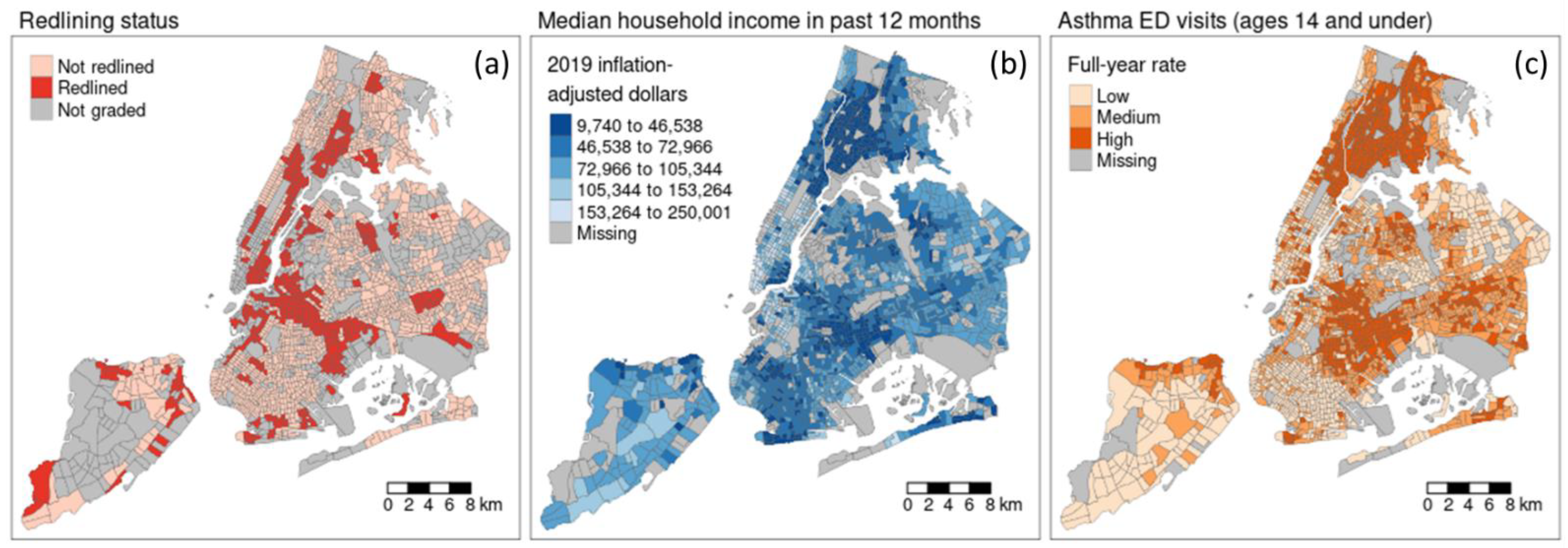
2.3. Equity Analysis

B-GLMMs were developed to examine differences in pollution exposure by redlining status and rate of pediatric asthma ED visits. Redlining status was determined by overlaying census tract geographies obtained from IPUMS NHGIS [38] and a digitized version of the HOLC map obtained from the University of Richmond Mapping Inequality Project [9]. For this analysis, a census tract was considered to have been redlined if its centroid intersected with a D-graded area on the HOLC map (Figure 1a). Since large sections of NYC were excluded from the HOLC map, the redlining analysis was restricted to census tracts with centroids that intersected with a HOLC-graded area. The asthma morbidity analysis was also performed using the census tract geography. Data on full-year and quarterly asthma ED visits were obtained from the New York Statewide Planning and Research Cooperative System for the period 2016–2018. NYC population data were obtained from the 2017–2021 American Community Survey [39]. Three-year rates of asthma ED visits in each census tract were calculated for children 14 years of age and younger and then grouped into tertiles (low, medium, high) (Figure 1c).
Associations among each of five pollutants (NO2, PM2.5, BC, V, Cu, Ni) and two demographic variables (redlining status and rate of pediatric asthma ED visits) were analyzed using B-GLMMs, controlling for year of study with random intercept to account for within-geography correlation and stratified by season and period—the study period was divided into pre-2016 (2008–2015) and post-2016 (2016–2019) periods, marking the dramatic shift in local air pollution trends resulting from multiple policies enacted prior to 2016 regulating emissions from residual fuel oil, electric generating units, and motor vehicles (Figure 2) [40]. This is apparent in the sharp change in slope in annual pollutant trends, where 2016 marks the inflection point when reductions in NO2 and PM2.5 start to plateau (Figure 2). While it is difficult to disentangle the effects of multiple, concurrent pollution regulations on the observed trends, we take the 2016 inflection point to be a marker of two periods having distinct pollution emission patterns and model them separately. The B-GLMMs assumed gamma-distributed dependent variables to reflect the skewed distribution of pollutant concentrations. The identity link was used so that covariate effect sizes could be interpreted in the original units of pollutant concentration. Typically, air pollution models are log-transformed to coerce skewed data into approximately normal distributions, yielding results in units of percent difference; percent differences can be misleading when used to compare differences in exposure among groups over time if overall exposure levels change dramatically over the study period as they do in our study. Thus, we used B-GLMMs to determine absolute differences in pollutant exposure among our study groups in order to produce clear and informative results. In contrast to a frequentist GLM, the Bayesian framework allows the setting of initial values for model fitting—this aided in model convergence when specifying the relatively restrictive gamma distribution. Weakly informative priors, based on observed data, were specified for model parameters. B-GLMMs were fit via MCMC estimation using the NIMBLE package [41] in R version 4.2.3 [36].

3. Results and Discussion

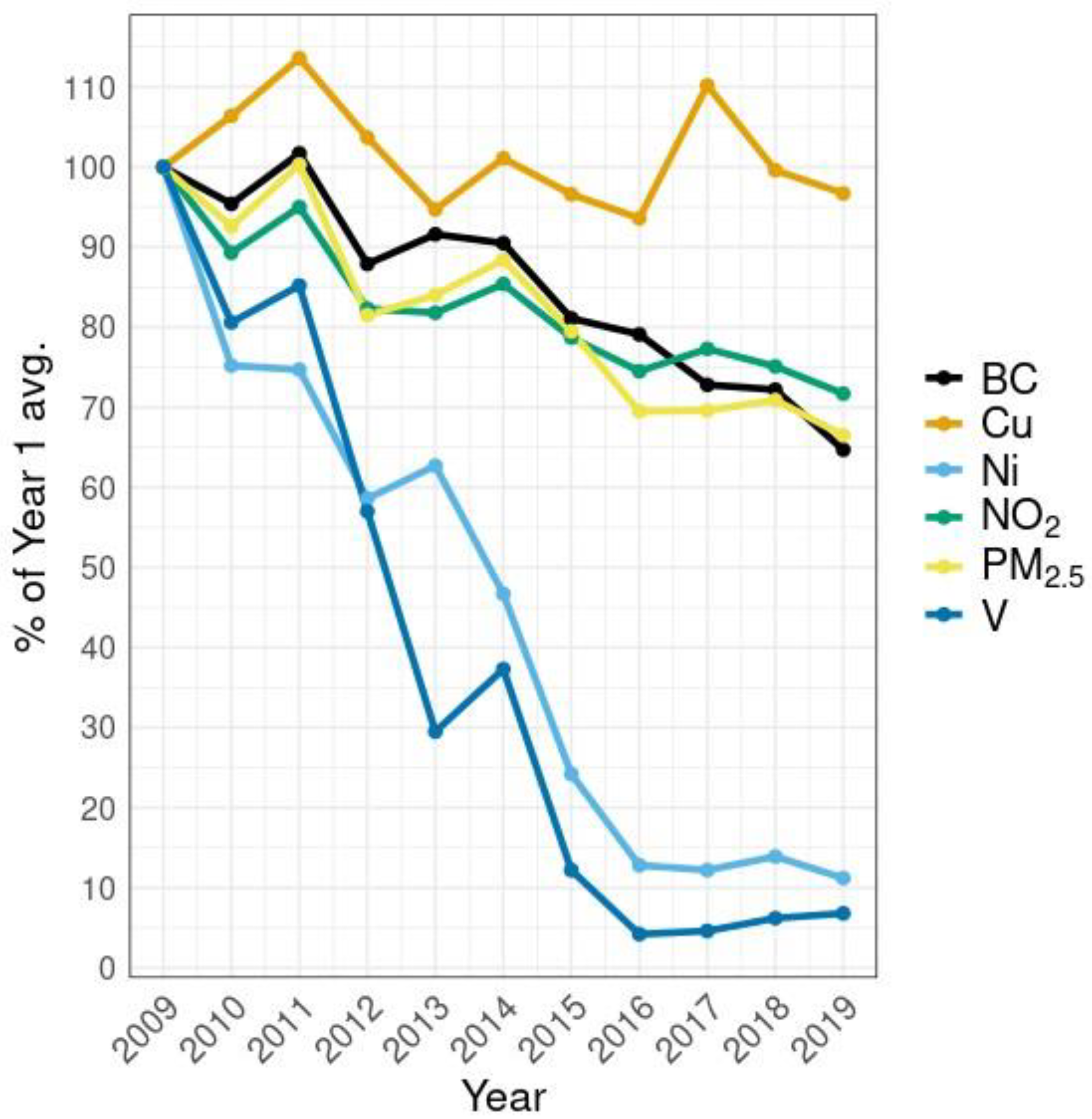
3.1. Temporal Trends in Citywide Air Pollution

Policies and events regulating emissions from residual fuel oil, electric generating units, and motor vehicles resulted in decreased PM2.5 and NO2 concentrations citywide [40]. From 2008 to 2019 PM2.5 fell from 12.8 to 8.51 µg/m3, NO2 fell from 27.8 to 19.9 ppb, BC fell from 1300 to 840 ng/m3, Ni fell from 8.44 to 0.947 ng/m3, V fell from 5.35 to 0.363 ng/m3, and Cu remained relatively constant at around 7 ng/m3 (Figure 2 and Figure 3).

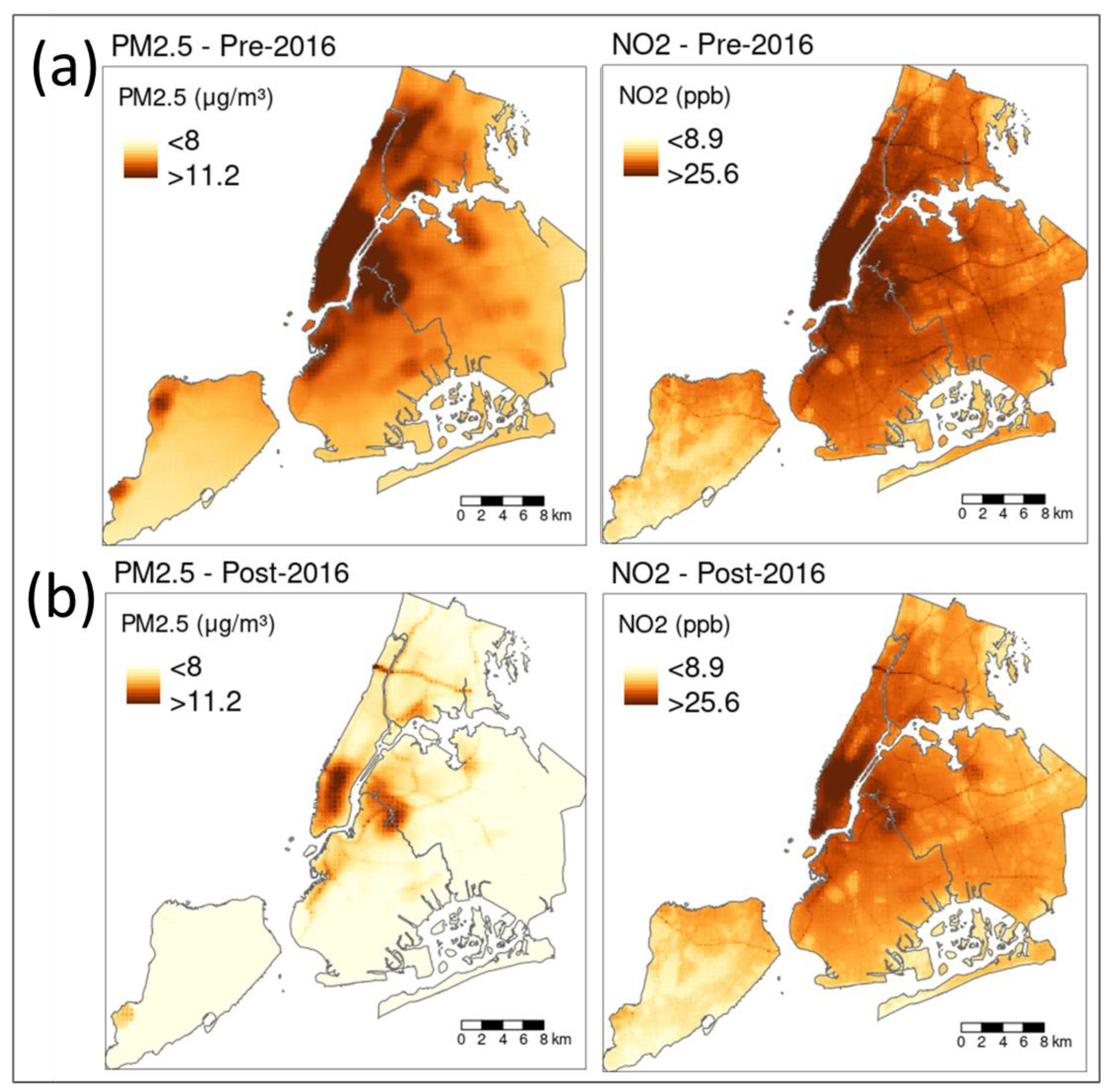
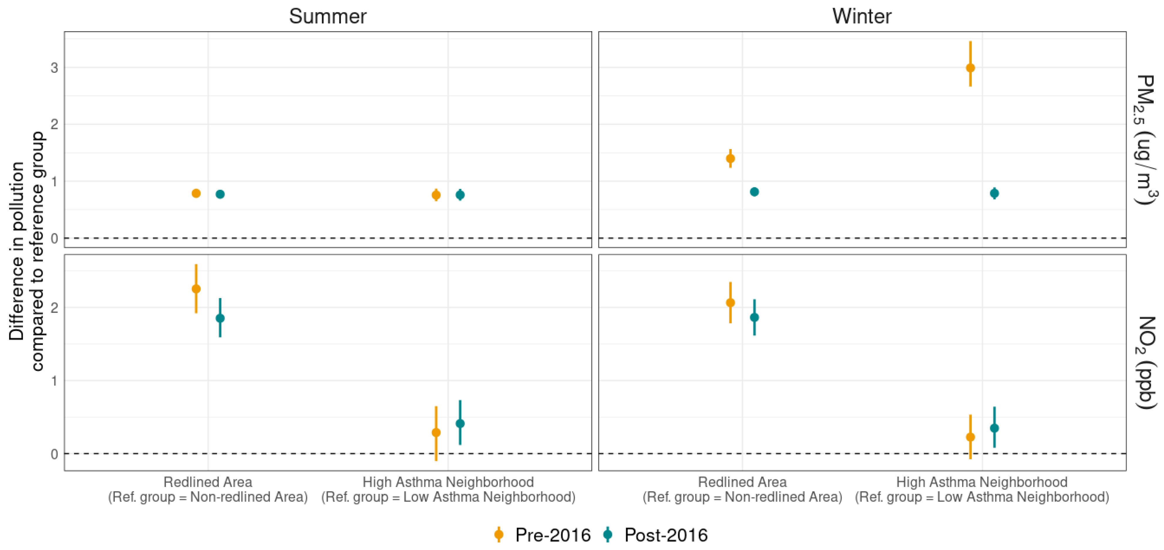
3.2. Spatial Disparities in NO2 and Total PM2.5 Exposure

Our B-GLMMs showed that, despite citywide declines, disparities endured in outdoor air pollution among neighborhoods with varying redlining statuses and rates of pediatric asthma ED visits. In the pre-2016 period, high-asthma neighborhoods experienced, on average, 0.76 [95% credible interval 0.65–0.87] µg/m3, 3.0 [2.7–3.5] µg/m3, 0.29 [−0.10–0.65] ppb, and 0.23 [−0.08–0.53] ppb higher levels of summertime PM2.5, wintertime PM2.5, summertime NO2, and wintertime NO2, respectively, compared to low-asthma neighborhoods (Figure 4). In the pre-2016 period, redlined areas experienced, on average, 0.79 [0.71–0.87] µg/m3, 1.4 [1.2–1.6] µg/m3, 2.3 [1.9–2.6] ppb, and 2.1 [1.8–2.3] ppb higher levels of summertime PM2.5, wintertime PM2.5, summertime NO2, and wintertime NO2, respectively, compared to areas that were not redlined (Figure 4). In the post-2016 period, high-asthma neighborhoods experience, on average, 0.76 [0.66–0.86] µg/m3, 0.79 [0.68–0.89] µg/m3, 0.41 [0.12–0.73] ppb, and 0.35 [0.08–0.64] ppb higher levels of summertime PM2.5, wintertime PM2.5, summertime NO2, and wintertime NO2, respectively, compared to low-asthma neighborhoods (Figure 4). In the post-2016 period, redlined areas experienced, on average, 0.77 [0.69–0.85] µg/m3, 0.81 [0.73–0.89] µg/m3, 1.9 [1.6–2.1] ppb, and 1.9 [1.6–2.1] ppb higher levels of summertime PM2.5, wintertime PM2.5, summertime NO2, and wintertime NO2, respectively, compared to areas that were not redlined (Figure 4). Lane et al. (2022) also reported nationwide disparities by redlining status using LUR-modeled pollutant surfaces based on US EPA regulatory monitor and satellite data from 2010 [5]. Recent studies have found that having lower socioeconomic status was associated with higher exposures to criteria air pollutants in cities around the world [42,43,44,45,46,47]. A study of NO2 in nine European cities observed higher NO2 among local administrative units having higher crime or unemployment rates, suggesting a positive association between air pollution and deprivation [48]. There is evidence that these inequities are growing larger, especially in developing nations in East and South Asia [47]. To our knowledge, ours is the first study to identify specific sources of air pollution exposure inequities using high-resolution PM2.5 constituent data based on a dense network of ground-based observations. In the following sections, we analyze trends in PM2.5 constituents to elucidate the underlying sources of inequity in NYC.

3.3. Source-Specific Exposure Trends
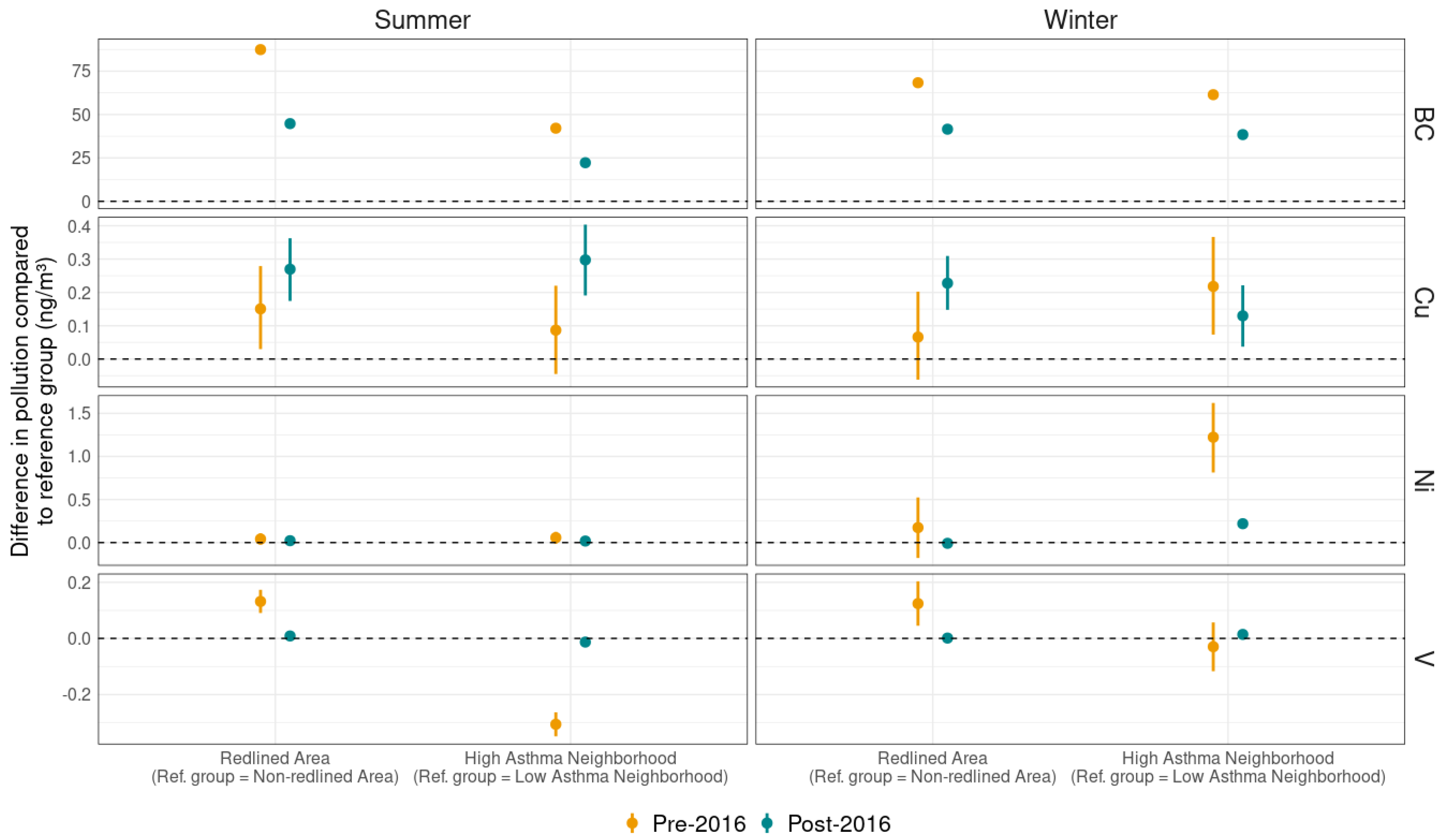
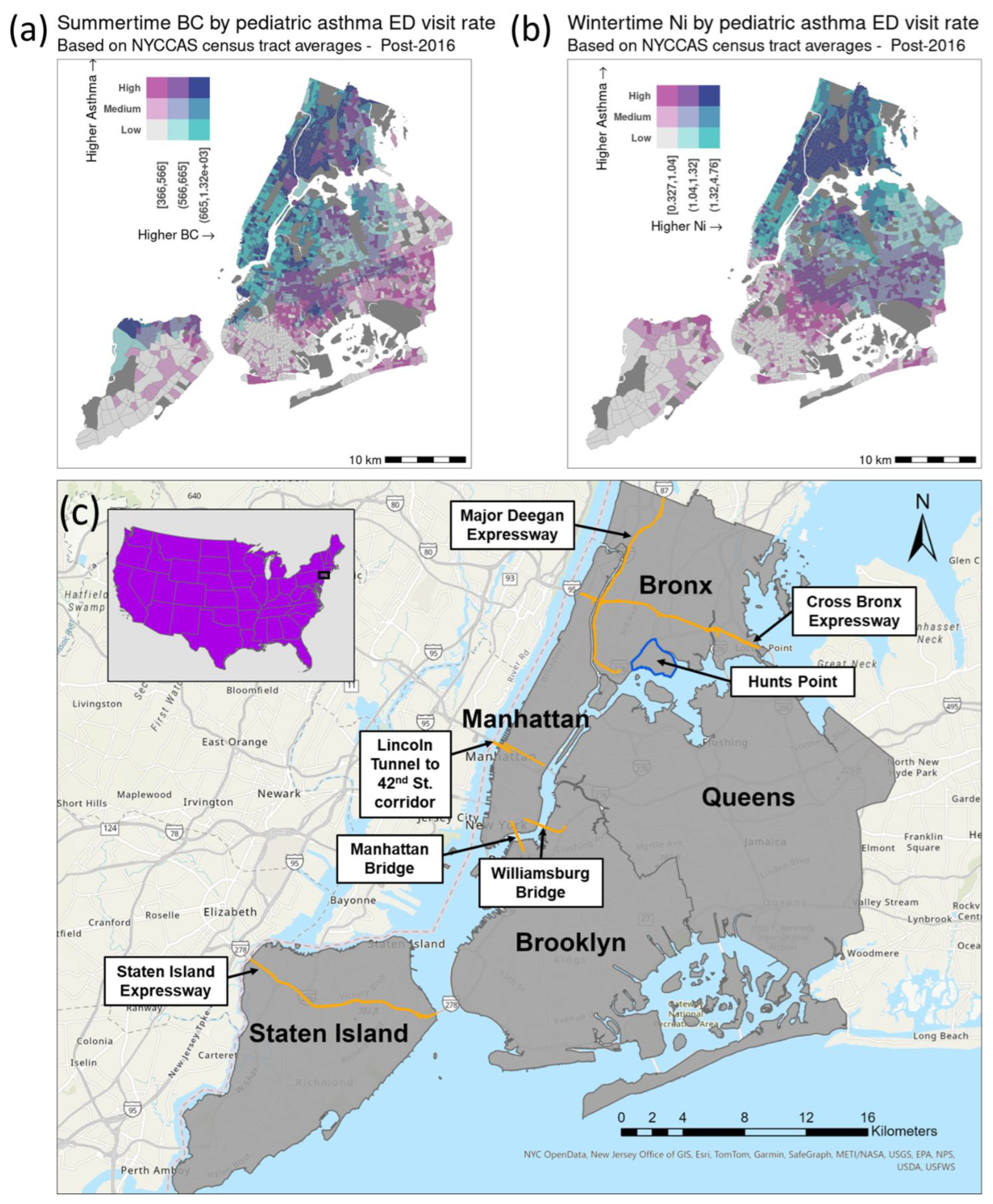
3.3.1. Traffic

Cu is highly associated with local traffic sources in NYC [25], reflecting non-exhaust emissions from brake wear [49]. Thus, fine particulate Cu patterns are driven by trends in traffic volume. BC is associated with and commonly used as a marker for diesel truck traffic emissions [32,50]. NYC traffic is often higher in the summer due to tourism and outdoor recreation [51], and the peak season for heavy-duty freight traffic (August–October, when retailers are stocking up for back-to-school and holiday shopping) overlaps the summer season [52]. This means that summertime patterns of traffic-related air pollution (i.e., Cu, BC) are likely dominated by traffic, as opposed to other shared sources, such as residual oil boilers (which have peak usage in winter for heating). Increasingly positive associations between summertime Cu and redlining (pre-2016: 0.15 [0.03–0.28] ng/m3 higher in redlined areas; post-2016: 0.27 [0.17–0.36] ng/m3 higher in redlined areas), as well as neighborhood pediatric asthma rates (pre-2016: 0.09 [−0.04–0.22] ng/m3 higher in high-asthma neighborhoods; post-2016: 0.30 [0.19–0.40] ng/m3 higher in high-asthma neighborhoods), indicate persistent disparities in neighborhood traffic volumes (Figure 5).
Furthermore, the differences in summertime BC by both redlining status (pre-2016: 87 [85–89] ng/m3 higher in redlined areas; post-2016: 45 [43–46] ng/m3 higher in redlined areas) and neighborhood asthma (pre-2016: 42 [40–44] ng/m3 higher in high-asthma neighborhoods; post-2016: 22 [21–24] ng/m3 higher in high-asthma neighborhoods) remain positive through both study periods, suggesting heavy-duty diesel vehicles as an enduring source of exposure disparities. Regulations on vehicle exhaust emissions may explain why summer BC disparities are decreasing as summer Cu disparities increase since BC is emitted in vehicle exhaust and Cu is not. These trends suggest that vehicle emissions controls have helped to reduce inequitable exposures to traffic-related pollution even as disparities in traffic volume appear to grow.

3.3.2. Residual Oil Boilers

While Ni has the strongest association with residual oil boilers in NYC [25], BC, V, and Cu are also associated with this source [25,50]. Building boilers operate year-round to produce hot water; however, their emissions are highest during the winter, when space heating reaches a peak. Wintertime differences by redlining status were virtually eliminated for Ni (0.17 [−0.18–0.52] to −0.0090 [−0.046–0.027]) and V (0.12 [0.045–0.20] to 0.0013 [−0.010–0.013]), and reduced for BC (68 [66–70] to 42 [40–43] ng/m3) between the two study periods, suggesting that regulations on boiler fuels had an equalizing effect on residual oil emissions (Figure 5). In NYC, a suite of “Clean Heat” policies mandated the phase-out of No. 6 fuel oil by 2015 and No. 4 oil by 2030 and reduced maximum allowable sulfur levels in No. 2 and No. 4 heating oils as of 2012 [53]. Differences in wintertime Cu, however, increased in redlined vs. non-redlined areas between the two study periods (0.066 [−0.062–0.20] to 0.23 [0.15–0.31] ng/m3). While Cu is a known component of residual oil emissions [54], it is most highly associated with traffic in NYC [25]. This suggests that variation in traffic emissions was sharper than variation in residual oil boiler emissions among neighborhoods of varying redlining status, so reductions in boiler emissions revealed the magnitude of the traffic emissions disparity. In other words, the wintertime Cu disparity by redlining appeared to be driven by traffic rather than residual oil emissions.
Our B-GLMMs also showed reduced disparities in high-asthma compared to low-asthma neighborhoods between the two study periods in wintertime Ni (1.22 [0.81–1.6] to 0.22 [0.18–0.26] ng/m3), wintertime BC (61 [59–63] to 38 [37–40] ng/m3), and wintertime Cu (0.22 [0.073–0.37] to 0.13 [0.037–0.22] ng/m3) (Figure 5), suggesting reduced exposure inequity to residual oil boiler emissions. However, the persistence of the Ni disparity suggests that, though Clean Heat improved air quality citywide [55], these policies did not eliminate inequitable exposure to residual oil boilers in high-asthma neighborhoods.

3.3.3. Marine Residual Oil

V exhibits the strongest association with marine residual oil emissions in NYC [25], though it is also a known component of residual oil used to fuel building boilers [54]. The high season for recreational cruise ships in NYC is summer [27], and peak container ship season follows that of freight trucking (August–October), driven by anticipated increases in demand during the holiday shopping season [26]. Thus, summertime V patterns are likely driven by marine residual oil emissions. Summertime V trends suggest drastically reduced marine residual oil emissions in redlined areas (pre-2016: 0.13 [0.091–0.17] ng/m3 higher in redlined areas; post-2016: 0.0088 [0.0024–0.015] ng/m3 higher in redlined areas). This may be due to decreased marine residual oil emissions in response to policies regulating the sulfur content of marine fuel oil that was phased in from the early 2000s to the mid-2010s [56,57]. In contrast to the findings for redlined areas, the spatial patterns of V suggest that marine residual oil is not a major source of disparate air pollution exposure in high-asthma neighborhoods (Figure 5).

3.4. Policy Implications

Over the study period, disparities in outdoor PM2.5 and NO2 exposure endured among neighborhoods with varying redlining status and rates of pediatric asthma ED visits. These disparities are, however, small relative to citywide average exposures (8.5 µg/m3 and 20 ppb for PM2.5 and NO2, respectively, in 2019), with PM2.5 disparities by both asthma morbidity and redlining amounting to approximately 0.8 µg/m3 and NO2 disparities by asthma and redlining amounting to <2 ppb in the post-2016 period. In acknowledging the disparities’ small magnitude, we seek not to diminish injustices, but rather to guide effective policy. Given small exposure disparities, concentrated efforts to reduce exposures in populations experiencing disproportionate health impacts would be more effective than focusing solely on where exposure disparities are greatest. The health benefits of continuing to reduce air pollution will be greater in high-asthma neighborhoods because of the association of outdoor PM2.5 and NO2 pollution with asthma exacerbation, including increased rates of pediatric asthma ED visits [19,20,21,58]. This study aimed to determine the sources of inequitable exposures among disproportionately impacted populations. While there is some overlap between high-asthma and redlined neighborhoods, differences in pollution trends (i.e., NO2 disparities decreasing in redlined areas but increasing in high-asthma neighborhoods) suggest that asthma morbidity may be a more useful proxy for community-level burden as neighborhood demographics shift.
Persistent disparities in wintertime PM2.5 constituent data suggest that benefits from Clean Heat policies have been insufficient to address inequities in air quality among neighborhoods with varying asthma morbidity rates. This is in contrast to redlined areas, which saw a virtual elimination of disparities in exposure to residual oil boilers. This may reflect shifting neighborhood demographics as some previously redlined areas become higher-income neighborhoods (Figure 1a,b). Building emissions can change as new developments replace older ones and existing buildings change fuel types—events that may be more likely in neighborhoods experiencing this demographic shift. NYC has undergone drastic neighborhood demographic shifts since the time of redlining as the city increased in population [59] and developers have sought to transform historically marginalized neighborhoods into more upscale ones [60]. As a result, redlining has become a less meaningful characteristic for identifying neighborhoods currently experiencing the most environmental injustice in NYC.
Compared to real estate development, traffic infrastructure is slower to change, and traffic emissions persist as a source of inequitable exposures in both high-asthma and redlined communities, including evidence suggesting increasing inequities. Increased summer Cu disparities point to increasingly inequitable exposures to traffic volume while decreased summer BC disparities indicate shrinking inequities in exposure to traffic emissions. Because traffic-related Cu is a non-exhaust emission and BC is an exhaust emission, these opposing trends suggest that regulations on vehicle exhaust emissions have, to some extent, offset the effects of a widening gap in traffic exposure among high- and low-traffic neighborhoods. While historic siting of traffic infrastructure has kept spatial patterns in traffic generally consistent, high-traffic neighborhoods may be experiencing disproportionate increases in truck traffic due to the rise in e-commerce [61,62], which relies on industrial hubs that are often in predominantly Black, Hispanic/Latino, and low-income neighborhoods [63].
To fully address environmental health inequities, we must tackle disparities in housing quality, indoor air quality, and access to healthcare in addition to outdoor air pollution [4,6]. The neighborhoods with the highest levels of outdoor air pollution in NYC are some of the wealthiest and do not experience higher rates of air pollution-attributable health outcomes [17], showing that outdoor air pollution is only one of many determinants of health. NYC has a central business district that acts as a major hub of commercial activity for a large and dense metropolitan area. The presence of this commercial activity makes the CBD an expensive place to live despite the pollution it produces, resulting in highly affluent neighborhoods with the highest air pollution in the city and ample resources to manage personal health. Nevertheless, the CBD is an exception to a trend, and our study shows that, on average, NYC communities with higher rates of pediatric asthma ED visits are exposed to higher concentrations of outdoor NO2 and PM2.5 compared to low-asthma neighborhoods and that traffic and building boiler emissions are important local sources of this disparity.
This study shows how PM2.5 constituents can be used to identify communities experiencing the greatest impact from local air pollution and the main sources of disparity. Figure 6 shows bivariate maps plotting neighborhood pediatric asthma ED visit rates against LUR-predicted wintertime Ni (tracer for residual oil boiler emissions) and summertime BC (tracer for heavy-duty diesel truck emissions) in the post-2016 period.
The summertime BC map highlights high-asthma neighborhoods exposed to disproportionately high diesel fuel emissions in northern Manhattan, in the proximity of a few major roadways, and in industrial areas in northern Brooklyn and Hunts Point in the Bronx (Figure 6a,c and Figure S2a,b). The wintertime Ni map shows that most of the Bronx and northern Manhattan stand out as high-asthma neighborhoods with disproportionate exposure to residual oil boiler emissions (Figure 6b and Figure S2c). That residual oil boiler and traffic emissions continue to disproportionately impact high-asthma neighborhoods is relevant to the implementation of local, state, and federal greenhouse gas mitigation strategies, including building and vehicle electrification that will also have air quality co-benefits [64,65,66,67]. These burgeoning initiatives are an opportunity to support and accelerate emissions reductions in overburdened and under-resourced communities.

3.5. Strengths and Limitations

A strength of this study is the NYCCAS network’s high density of long-term, ground-level air pollution monitors. This gives us the ability to investigate highly resolved spatial variability in local sources as indicated by PM2.5 constituents shown to have robust associations with specific sources in NYC [25]. Though some of the PM2.5 constituents analyzed in this study are correlated with each other and show associations with multiple sources [24,25], we add specificity to our analysis by stratifying the B-GLMMs by season as there are strong seasonal patterns to the sources examined in this study. For example, residual oil boiler emissions peak in the winter heating season, and marine residual oil emissions peak in summer [26,27]. One weakness of the NYCCAS dataset is its temporal resolution, which is limited to seasonal averages at each site (only winter and summer measurements for PM2.5 elemental constituents). This limited our ability to perform source apportionment, which typically requires high temporal resolution data in order to effectively resolve distinct source factors. To our knowledge, conventional source apportionment methods, such as Positive Matrix Factorization, have not been used to resolve neighborhood-level patterns in local sources because they typically rely on highly temporally resolved data collected from sparsely distributed sites [28,29,30]. Other recent studies of air pollution exposure inequities using LUR [5], source-receptor models [7], or satellite-based data [3,68] similarly observed disparities in air pollution exposure by redlining, race, ethnicity, and income. However, these studies were limited to analyses of total PM2.5 or NO2. As far as we know, ours is the first study to identify specific sources of air pollution exposure inequities on the neighborhood level using high-resolution PM2.5 constituent data from a dense network of ground-based observations.

4. Conclusions

Redlined areas experienced near elimination of disparities in exposure to residual oil boilers and marine residual oil, with persistent inequitable exposures to traffic. High-asthma neighborhoods continue to have disproportionately higher exposures to both traffic and residual oil emissions. These differences in trend suggest that the spatial pattern of asthma morbidity may be a more useful proxy for community-level burden as neighborhood demographics shift (Figure 1). Though addressing outdoor air pollution levels helps to reduce exacerbation, asthma is a complex condition driven mainly by factors that are addressed through improved economic opportunity, access to healthcare, and housing quality [6,69,70]—factors potentially supported by well-designed and equitable climate policies [67]. While there is evidence of inequities in air pollution exposure in cities outside of the United States [42,43,45,46,47,48], these studies are relatively limited in number and scope [42,44], with few investigating specific pollution sources contributing to inequity. Other municipalities may also want to use the methods in this study to analyze spatial patterns of chemical source indicators to reveal sources of exposure inequity. This will become possible for more places as spatially resolved air pollution constituent data becomes more widely available via current and upcoming satellite missions, such as TEMPO [71] and MAIA [31]. Regardless of the granularity in air pollution surveillance, local policymakers in NYC and other cities should consider the spatial patterns of health disparities in designing air quality policy that supports environmental justice and maximizes health benefits. Because overall exposure disparities in NYC are small, our findings suggest that pollution policy in NYC should focus on reducing traffic and building boiler emissions in high-asthma neighborhoods to reduce exacerbations.

Supplementary Materials

The following supporting information can be downloaded at: https://www.mdpi.com/article/10.3390/pollutants5010002/s1, Figure S1: NYCCAS integrated two-week monitoring sites. The core sites (dark blue circles and triangles) have been monitored every year since the inception of NYCCAS (December 2008). The number of reference sites (triangles) was reduced from 5 to 3 after Year 5 of NYCCAS; Figure S2: Spatial distribution of (a) annual average daily truck volumes, (b) industrial land use, and (c) buildings burning No. 4 fuel oil in NYC. Truck traffic data was obtained from the New York State Department of Transportation. Industrial land use data was obtained from the NYC Department of City Planning. Data on fuel oil permits was obtained from the NYC Mayor’s Office of Climate and Environmental Justice; Figure S3: Spatial patterns of PM2.5 in different seasons and study periods by census tract; Figure S4: Spatial patterns of NO2 in different seasons and study periods by census tract; Figure S5: Spatial patterns of BC in different seasons and study periods by census tract; Figure S6: Spatial patterns of Cu in different seasons and study periods by census tract; Figure S7: Spatial patterns of Ni in different seasons and study periods by census tract; Figure S8: Spatial patterns of V in different seasons and study periods by census tract; Figure S9: Bivariate maps of PM2.5 and pediatric asthma emergency department visit rate in different seasons and study periods by census tract. Asthma rates were not available for census tracts colored in dark gray. Map legends show the ranges of PM2.5 concentrations for each color bin in units of micrograms per cubic meter (µg/m3); Figure S10: Bivariate maps of NO2 and pediatric asthma emergency department visit rate in different seasons and study periods by census tract. Asthma rates were not available for census tracts colored in dark gray. Map legends show the ranges of NO2 concentrations for each color bin in units of parts per billion (ppb); Figure S11: Bivariate maps of BC and pediatric asthma emergency department visit rate in different seasons and study periods by census tract. Asthma rates were not available for census tracts colored in dark gray. Map legends show the ranges of BC concentrations for each color bin in units of nanograms per cubic meter (ng/m3); Figure S12: Bivariate maps of Cu and pediatric asthma emergency department visit rate in different seasons and study periods by census tract. Asthma rates were not available for census tracts colored in dark gray. Map legends show the ranges of Cu concentrations for each color bin in units of nanograms per cubic meter (ng/m3); Figure S13: Bivariate maps of Ni and pediatric asthma emergency department visit rate in different seasons and study periods by census tract. Asthma rates were not available for census tracts colored in dark gray. Map legends show the ranges of Ni concentrations for each color bin in units of nanograms per cubic meter (ng/m3); Figure S14: Bivariate maps of V and pediatric asthma emergency department visit rate in different seasons and study periods by census tract. Asthma rates were not available for census tracts colored in dark gray. Map legends show the ranges of V concentrations for each color bin in units of nanograms per cubic meter (ng/m3); Figure S15: Bivariate maps of PM2.5 and redlining status in different seasons and study periods by census tract. Census tracts whose centroids did not overlap with a HOLC-graded area are represented in dark gray. Map legends show the ranges of PM2.5 concentrations for each color bin in units of micrograms per cubic meter (µg/m3); Figure S16: Bivariate maps of NO2 and redlining status in different seasons and study periods by census tract. Census tracts whose centroids did not overlap with a HOLC-graded area are represented in dark gray. Map legends show the ranges of NO2 concentrations for each color bin in units of parts per billion (ppb); Figure S17: Bivariate maps of BC and redlining status in different seasons and study periods by census tract. Census tracts whose centroids did not overlap with a HOLC-graded area are represented in dark gray. Map legends show the ranges of BC concentrations for each color bin in units of nanograms per cubic meter (ng/m3); Figure S18: Bivariate maps of Cu and redlining status in different seasons and study periods by census tract. Census tracts whose centroids did not overlap with a HOLC-graded area are represented in dark gray. Map legends show the ranges of Cu concentrations for each color bin in units of nanograms per cubic meter (ng/m3); Figure S19: Bivariate maps of Ni and redlining status in different seasons and study periods by census tract. Census tracts whose centroids did not overlap with a HOLC-graded area are represented in dark gray. Map legends show the ranges of Ni concentrations for each color bin in units of nanograms per cubic meter (ng/m3); Figure S20: Bivariate maps of V and redlining status in different seasons and study periods by census tract. Census tracts whose centroids did not overlap with a HOLC-graded area are represented in dark gray. Map legends show the ranges of V concentrations for each color bin in units of nanograms per cubic meter (ng/m3); Table S1: Data sources and interpretation of emissions indicators used in land-use regression models; Table S2: Selected land-use regression models, R-squared, and normalized mean squared error (NMSE) for PM2.5 in Years 1–11 of the New York City Community Air Survey. See Table S1 for interpretation of emissions indicators. (n = number of monitoring sites included in model; conc = pollutant concentration; datenum = unique 2-week sampling session ID; season_sort = unique season-year ID); Table S3: Selected land-use regression models, R-squared, and normalized mean squared error (NMSE) for NO2 in Years 1–11 of the New York City Community Air Survey. See Table S1 for interpretation of emissions indicators. (n = number of monitoring sites included in model; conc = pollutant concentration; datenum = unique 2-week sampling session ID; season_sort = unique season-year ID); Table S4: Selected land-use regression models, R-squared, and normalized mean squared error (NMSE) for BC in Years 1–11 of the New York City Community Air Survey. See Table S1 for interpretation of emissions indicators. (n = number of monitoring sites included in model; conc = pollutant concentration; datenum = unique 2-week sampling session ID; season_sort = unique season-year ID); Table S5: Selected land-use regression models, R-squared, and normalized mean squared error (NMSE) for Cu in Years 1–11 of the New York City Community Air Survey. See Table S1 for interpretation of emissions indicators. (n = number of monitoring sites included in model; conc = pollutant concentration; datenum = unique 2-week sampling session ID; season_sort = unique season-year ID); Table S6: Selected land-use regression models, R-squared, and normalized mean squared error (NMSE) for Ni in Years 1–11 of the New York City Community Air Survey. See Table S1 for interpretation of emissions indicators. (n = number of monitoring sites included in model; conc = pollutant concentration; datenum = unique 2-week sampling session ID; season_sort = unique season-year ID); Table S7: Selected land-use regression models, R-squared, and normalized mean squared error (NMSE) for V in Years 1–11 of the New York City Community Air Survey. See Table S1 for interpretation of emissions indicators. (n = number of monitoring sites included in model; conc = pollutant concentration; datenum = unique 2-week sampling session ID; season_sort = unique season-year ID).

Author Contributions

M.P.: Conceptualization, Methodology, Formal analysis, Visualization, Writing—Original Draft. S.J.: Conceptualization, Methodology, Writing—Review and Editing, Supervision. A.S.-C.: Data Curation, Writing—Review and Editing. H.E.: Investigation, Writing—Review and Editing. K.I.: Methodology, Writing—Review and Editing, Supervision. All authors have read and agreed to the published version of the manuscript.

Funding

This work was supported by the City of New York tax levy funds and New York State Energy Research and Development Authority (NYSERDA) agreement number 156225, and we thank our NYSERDA program manager Ellen Burkhard. Any opinions expressed in this article do not necessarily reflect those of NYSERDA or the State of New York.

Data Availability Statement

This publication was produced from raw data purchased from or provided by the New York State Department of Health (NYSDOH). However, the calculations, metrics, conclusions derived, and views expressed herein are those of the author(s) and do not reflect the conclusions or views of NYSDOH. NYSDOH, its employees, officers, and agents make no representation, warranty, or guarantee as to the accuracy, completeness, currency, or suitability of the information provided here. Because of slight variations between datasets, results might differ from those calculated using a different extract of the NYSDOH Statewide Planning and Research Cooperative System (SPARCS). This analysis includes data from SPARCS 2016–2018, which were cut by NYSDOH in January 2023. Internal analyses by the NYC Department of Health and Mental Hygiene were conducted in July 2023. With the exception of raw SPARCS data, which comprises protected health information, the raw data supporting the conclusions of this article will be made available by the authors on request.

Acknowledgments

Previous versions of the manuscript were improved by thoughtful comments from Carolyn Olson (NYC Department of Health and Mental Hygiene). The authors also thank Nalyn Siripanichgon (Queens College), Christopher Huskey (NYC Department of Health and Mental Hygiene), and the rest of the NYCCAS team for collecting and curating the air pollution data used in this study.

Conflicts of Interest

The authors declare no conflicts of interest.

References

  1. World Health Organization (WHO). Ambient (Outdoor) Air Pollution. 2024. Available online: https://www.who.int/news-room/fact-sheets/detail/ambient-(outdoor)-air-quality-and-health (accessed on 5 November 2024).
  2. US Environmental Protection Agency (USEPA). Our Nation’s Air: Trends Through 2021. 2022. Available online: https://gispub.epa.gov/air/trendsreport/2022/#home (accessed on 17 May 2023).
  3. Demetillo, M.A.G.; Harkins, C.; McDonald, B.C.; Chodrow, P.S.; Sun, K.; Pusede, S.E. Space-Based Observational Constraints on NO2 Air Pollution Inequality From Diesel Traffic in Major US Cities. Geophys. Res. Lett. 2021, 48, e2021GL094333. [Google Scholar] [CrossRef]
  4. Ferguson, L.; Taylor, J.; Davies, M.; Shrubsole, C.; Symonds, P.; Dimitroulopoulou, S. Exposure to indoor air pollution across socio-economic groups in high-income countries: A scoping review of the literature and a modelling methodology. Environ. Int. 2020, 143, 105748. [Google Scholar] [CrossRef]
  5. Lane, H.M.; Morello-Frosch, R.; Marshall, J.D.; Apte, J.S. Historical Redlining Is Associated with Present-Day Air Pollution Disparities in U.S. Cities. Environ. Sci. Technol. Lett. 2022, 9, 345–350. [Google Scholar] [CrossRef]
  6. NYC Department of Health and Mental Hygiene (NYCDOHMH). Childhood Asthma and the Asthma Counselor Program of the East Harlem Asthma Center of Excellence. 2017. Available online: https://www.nyc.gov/assets/doh/downloads/pdf/epi/databrief90.pdf (accessed on 7 June 2022).
  7. Tessum, C.W.; Paolella, D.A.; Chambliss, S.E.; Apte, J.S.; Hill, J.D.; Marshall, J.D. PM2. 5 polluters disproportionately and systemically affect people of color in the United States. Sci. Adv. 2021, 7, eabf4491. [Google Scholar] [CrossRef] [PubMed]
  8. NYC Department of Health and Mental Hygiene (NYCDOHMH). Health, Housing, and History. 2021. Available online: https://a816-dohbesp.nyc.gov/IndicatorPublic/data-stories/housing/ (accessed on 17 May 2023).
  9. Nelson, R.K.; Winling, L.; Marciano, R.; Connolly, N. Mapping Inequality; Nelson, R.K., Ayers, E.L., Eds.; American Panorama; Digital Scholarship Lab, University of Richmond: Richmond, VA, USA, 2023; Available online: https://dsl.richmond.edu/panorama/redlining (accessed on 9 June 2022).
  10. NYC Department of Health and Mental Hygiene (NYCDOHMH). Health Impacts of Air Pollution. 2022. Available online: https://a816-dohbesp.nyc.gov/IndicatorPublic/data-explorer/health-impacts-of-air-pollution/?id=2117#display=summary (accessed on 17 May 2023).
  11. New York State Department of Health (NYSDOH). Asthma Study—A Response to Budget Article VII, 2018–2019 SFY. 2023. Available online: https://www.health.ny.gov/statistics/ny_asthma/pdf/2018-2019_asthma_burden_nyc.pdf (accessed on 2 January 2025).
  12. Khan, S.; Bajwa, S.; Brahmbhatt, D.; Lovinsky-Desir, S.; Sheffield, P.E.; Stingone, J.A.; Li, S. Multi-level socioenvironmental contributors to childhood asthma in New York City: A cluster analysis. J. Urban Health 2021, 98, 700–710. [Google Scholar] [CrossRef] [PubMed]
  13. NYC Department of Health and Mental Hygiene (NYCDOHMH). Health Impacts of Air Pollution. 2022. Available online: https://a816-dohbesp.nyc.gov/IndicatorPublic/data-explorer/health-impacts-of-air-pollution/?id=2108#display=links (accessed on 17 May 2023).
  14. Bowser, B.P.; Devadutt, C. (Eds.) Racial Inequality in New York City Since 1965; SUNY Press: Albany, NY, USA, 2019. [Google Scholar]
  15. Office of the New York City Comptroller (NYC Comptroller). The Racial Wealth Gap in New York. 2023. Available online: https://comptroller.nyc.gov/reports/the-racial-wealth-gap-in-new-york/ (accessed on 11 January 2024).
  16. Poverty Tracker Research Group at Columbia University (Poverty Tracker). The State of Poverty and Disadvantage in New York City. 2021. Volume 3. Available online: https://static1.squarespace.com/static/610831a16c95260dbd68934a/t/6113f3b27a11e63e811521a9/1628697527573/POVERTY_TRACKER_REPORT25.pdf (accessed on 11 January 2024).
  17. Kheirbek, I.; Wheeler, K.; Walters, S.; Kass, D.; Matte, T. PM2.5 and ozone health impacts and disparities in New York City: Sensitivity to spatial and temporal resolution. Air Qual. Atmos. Health 2013, 6, 473–486. [Google Scholar] [CrossRef] [PubMed]
  18. Pitiranggon, M.; Johnson, S.; Huskey, C.; Eisl, H.; Ito, K. Effects of the COVID-19 shutdown on spatial and temporal patterns of air pollution in New York City. Environ. Adv. 2022, 7, 100171. [Google Scholar] [CrossRef]
  19. Strickland, M.J.; Darrow, L.A.; Klein, M.; Flanders, W.D.; Sarnat, J.A.; Waller, L.A.; Sarnat, S.E.; Mulholland, J.A.; Tolbert, P.E. Short-term associations between ambient air pollutants and pediatric asthma emergency department visits. Am. J. Respir. Crit. Care Med. 2010, 182, 307–316. [Google Scholar] [CrossRef] [PubMed]
  20. US Environmental Protection Agency (USEPA). Integrated Science Assessment for Oxides of Nitrogen—Health Criteria. 2016. Available online: https://assessments.epa.gov/isa/document/&deid=310879 (accessed on 14 May 2021).
  21. US Environmental Protection Agency (USEPA). Integrated Science Assessment for Particulate Matter. 2019. Available online: https://www.epa.gov/isa/integrated-science-assessment-isa-particulate-matter (accessed on 14 May 2021).
  22. Taquechel, K.; Diwadkar, A.R.; Sayed, S.; Dudley, J.W.; Grundmeier, R.W.; Kenyon, C.C.; Henrickson, S.E.; Himes, B.E.; Hill, D.A. Pediatric asthma health care utilization, viral testing, and air pollution changes during the COVID-19 pandemic. J. Allergy Clin. Immunol. Pract. 2020, 8, 3378–3387. [Google Scholar] [CrossRef] [PubMed]
  23. Xu, S.; Glenn, S.; Sy, L.; Qian, L.; Hong, V.; Ryan, D.S.; Jacobsen, S. Impact of the COVID-19 pandemic on health care utilization in a large integrated health care system: Retrospective cohort study. J. Med. Internet Res. 2021, 23, e26558. [Google Scholar] [CrossRef] [PubMed]
  24. Hennigan, C.J.; Mucci, A.; Reed, B.E. Trends in PM2.5 transition metals in urban areas across the United States. Environ. Res. Lett. 2019, 14, 104006. [Google Scholar] [CrossRef]
  25. Ito, K.; Johnson, S.; Kheirbek, I.; Clougherty, J.; Pezeshki, G.; Ross, Z.; Eisl, H.; Matte, T.D. Intraurban Variation of Fine Particle Elemental Concentrations in New York City. Environ. Sci. Technol. 2016, 50, 7517–7526. [Google Scholar] [CrossRef]
  26. FREIGHTOS. Beating Peak Shipping Season. 2023. Available online: https://www.freightos.com/freight-resources/beating-peak-season-blues-shipping-freights-busiest-season/ (accessed on 8 May 2023).
  27. NYC Economic Development Corporation (NYC EDC). NYCRUISE. 2023. Available online: https://nycruise.com/ (accessed on 8 May 2023).
  28. Zhu, Q.; Liu, Y.; Hasheminassab, S. Long-term source apportionment of PM2. 5 across the contiguous United States (2000–2019) using a multilinear engine model. J. Hazard. Mater. 2024, 472, 134550. [Google Scholar] [CrossRef]
  29. Hopke, P.K.; Chen, Y.; Chalupa, D.C.; Rich, D.Q. Long term trends in source apportioned particle number concentrations in Rochester NY. Environ. Pollut. 2024, 347, 123708. [Google Scholar] [CrossRef]
  30. Squizzato, S.; Masiol, M.; Rich, D.Q.; Hopke, P.K. A long-term source apportionment of PM2.5 in New York State during 2005–2016. Atmos. Environ. 2018, 192, 35–47. [Google Scholar] [CrossRef]
  31. National Aeronautics and Space Administration (NASA). MAIA: New NASA Instrument to Study Air Pollution. 2023. Available online: https://maia.jpl.nasa.gov/ (accessed on 17 May 2023).
  32. Matte, T.D.; Ross, Z.; Kheirbek, I.; Eisl, H.; Johnson, S.; Gorczynski, J.E.; Kass, D.; Markowitz, S.; Pezeshki, G.; Clougherty, J.E. Monitoring intraurban spatial patterns of multiple combustion air pollutants in New York City: Design and implementation. J. Expo. Sci. Environ. Epidemiol. 2013, 23, 223–231. [Google Scholar] [CrossRef]
  33. NYC Department of Health and Mental Hygiene (NYCDOHMH). Appendix 1—Sampling Methodology and Data Sources for Emissions Indicators. 2021. Available online: https://nyccas.cityofnewyork.us/nyccas2021/web/sites/default/files/NYCCAS-appendix/Appendix1.pdf (accessed on 17 May 2023).
  34. Clougherty, J.E.; Kheirbek, I.; Eisl, H.M.; Ross, Z.; Pezeshki, G.; Gorczynski, J.E.; Johnson, S.; Markowitz, S.; Kass, D.; Matte, T. Intra-urban spatial variability in wintertime street-level concentrations of multiple combustion-related air pollutants: The New York City Community Air Survey (NYCCAS). J. Expo. Sci. Environ. Epidemiol. 2013, 23, 232–240. [Google Scholar] [CrossRef] [PubMed]
  35. Wood, S.N. Fast stable restricted maximum likelihood and marginal likelihood estimation of semiparametric generalized linear models. J. R. Stat. Soc. Ser. B 2011, 73, 3–36. [Google Scholar] [CrossRef]
  36. R Core Team. R: A Language and Environment for Statistical Computing; R Foundation for Statistical Computing: Vienna, Austria, 2023; Available online: https://www.R-project.org/ (accessed on 17 March 2022).
  37. US Environmental Protection Agency (USEPA). Evaluation of CMAQ Applications at Neighborhood Scales. 2024. Available online: https://www.epa.gov/cmaq/evaluation-cmaq-applications-neighborhood-scales (accessed on 2 January 2025).
  38. Manson, S.; Schroeder, J.; Van Riper, D.; Kugler, T.; Ruggles, S. IPUMS National Historical Geographic Information System: Version 17.0 [Dataset]; IPUMS: Minneapolis, MN, USA, 2022. [Google Scholar] [CrossRef]
  39. US Census Bureau (US Census). “S0101 Age and Sex”. 2017–2021 American Community Survey. U.S. Census Bureau’s American Community Survey Office. 2021. Available online: https://data.census.gov/table?q=S0101%20Age%20and%20Sex&g=050XX00US36005,36047,36061,36081,36085 (accessed on 12 April 2023).
  40. Pitiranggon, M.; Johnson, S.; Haney, J.; Eisl, H.; Ito, K. Long-term trends in local and transported PM2.5 pollution in New York City. Atmos. Environ. 2021, 248, 118238. [Google Scholar] [CrossRef]
  41. de Valpine, P.; Turek, D.; Paciorek, C.J.; Anderson-Bergman, C.; Temple Lang, D.; Bodik, R. Programming with models: Writing statistical algorithms for general model structures with NIMBLE. J. Comput. Graph. Stat. 2017, 26, 403–413. [Google Scholar] [CrossRef]
  42. Fairburn, J.; Schüle, S.A.; Dreger, S.; Karla Hilz, L.; Bolte, G. Social inequalities in exposure to ambient air pollution: A systematic review in the WHO European region. Int. J. Environ. Res. Public Health 2019, 16, 3127. [Google Scholar] [CrossRef]
  43. Fan, X.P.; Lam, K.C.; Yu, Q. Differential exposure of the urban population to vehicular air pollution in Hong Kong. Sci. Total Environ. 2012, 426, 211–219. [Google Scholar] [CrossRef] [PubMed]
  44. Hajat, A.; Hsia, C.; O’Neill, M.S. Socioeconomic disparities and air pollution exposure: A global review. Curr. Environ. Health Rep. 2015, 2, 440–450. [Google Scholar] [CrossRef] [PubMed]
  45. Pearce, J.; Kingham, S. Environmental inequalities in New Zealand: A national study of air pollution and environmental justice. Geoforum 2008, 39, 980–993. [Google Scholar] [CrossRef]
  46. Rooney, M.S.; Arku, R.E.; Dionisio, K.L.; Paciorek, C.; Friedman, A.B.; Carmichael, H.; Zhou, Z.; Hughes, A.F.; Vallarino, J.; Agyei-Mensah, S.; et al. Spatial and temporal patterns of particulate matter sources and pollution in four communities in Accra, Ghana. Sci Total Environ. 2012, 435, 107–114. [Google Scholar] [CrossRef] [PubMed]
  47. Yu, W.; Ye, T.; Chen, Z.; Xu, R.; Song, J.; Li, S.; Guo, Y. Global analysis reveals region-specific air pollution exposure inequalities. One Earth 2024, 7, 2063–2071. [Google Scholar] [CrossRef]
  48. Samoli, E.; Stergiopoulou, A.; Santana, P.; Rodopoulou, S.; Mitsakou, C.; Dimitroulopoulou, C.; Bauwelinck, M.; de Hoogh, K.; Costa, C.; Marí-Dell’Olmo, M.; et al. Spatial variability in air pollution exposure in relation to socioeconomic indicators in nine European metropolitan areas: A study on environmental inequality. Environ. Pollut. 2019, 249, 345–353. [Google Scholar] [CrossRef]
  49. Harrison, R.M.; Jones, A.M.; Gietl, J.; Yin, J.; Green, D.C. Estimation of the contributions of brake dust, tire wear, and resuspension to nonexhaust traffic particles derived from atmospheric measurements. Environ. Sci. Technol. 2012, 46, 6523–6529. [Google Scholar] [CrossRef] [PubMed]
  50. Cornell, A.G.; Chillrud, S.N.; Mellins, R.B.; Acosta, L.M.; Miller, R.L.; Quinn, J.W.; Yan, B.; Divjan, A.; Olmedo, O.E.; Lopez-Pintado, S.; et al. Domestic airborne black carbon and exhaled nitric oxide in children in NYC. J. Expo. Sci. Environ. Epidemiol. 2012, 22, 258–266. [Google Scholar] [CrossRef]
  51. Rattigan, O.V.; Civerolo, K.; Doraiswamy, P.; Felton, H.D.; Hopke, P.K. Long Term Black Carbon Measurements at Two Urban Locations in New York. Aerosol Air Qual. Res. 2013, 13, 1181–1196. [Google Scholar] [CrossRef]
  52. R2Logistics. The Ins and Outs of the Seasonality of Freight. 2022. Available online: https://www.r2logistics.com/the-ins-and-outs-of-the-seasonality-of-freight/ (accessed on 8 May 2023).
  53. Kheirbek, I.; Haney, J.; Douglas, S.; Ito, K.; Caputo, S., Jr.; Matte, T. The public health benefits of reducing fine particulate matter through conversion to cleaner heating fuels in New York City. Environ. Sci. Technol. 2014, 48, 13573–13582. [Google Scholar] [CrossRef] [PubMed]
  54. Huffman, G.P.; Huggins, F.E.; Shah, N.; Huggins, R.; Linak, W.P.; Miller, C.A.; Pugmire, R.J.; Meuzelaar, H.L.; Seehra, M.S.; Manivannan, A. Characterization of fine particulate matter produced by combustion of residual fuel oil. J. Air Waste Manag. Assoc. 2000, 50, 1106–1114. [Google Scholar] [CrossRef] [PubMed]
  55. Zhang, L.; He, M.Z.; Gibson, E.A.; Perera, F.; Lovasi, G.S.; Clougherty, J.E.; Carrion, D.; Burke, K.; Fry, D.; Kioumourtzoglou, M.A. Evaluating the Impact of the Clean Heat Program on Air Pollution Levels in New York City. Environ. Health Perspect. 2021, 129, 127701. [Google Scholar] [CrossRef]
  56. US Environmental Protection Agency (USEPA). International Standards to Reduce Emissions from Marine Diesel Engines and Their Fuels. 2019b. Available online: https://www.epa.gov/regulations-emissions-vehicles-and-engines/international-standards-reduce-emissions-marine-diesel (accessed on 17 May 2023).
  57. Winebrake, J.J.; Corbett, J.; Green, E.; Lauer, A.; Eyring, V. Mitigating the health impacts of pollution from oceangoing shipping: An assessment of low-sulfur fuel mandates. Environ. Sci. Technol. 2009, 43, 4776–4782. [Google Scholar] [CrossRef]
  58. Bi, J.; D’Souza, R.R.; Moss, S.; Senthilkumar, N.; Russell, A.G.; Scovronick, N.C.; Chang, H.H.; Ebelt, S. Acute effects of ambient air pollution on asthma emergency department visits in ten US States. Environ. Health Perspect. 2023, 131, 047003. [Google Scholar] [CrossRef] [PubMed]
  59. NYC Department of City Planning (NYCDCP). New York City’s Current Population Estimates and Trends. 2023. Available online: https://www.nyc.gov/assets/planning/download/pdf/planning-level/nyc-population/population-estimates/population-trends-2022.pdf?r=a (accessed on 12 January 2024).
  60. NYU Furman Center. State of New York City’s Housing and Neighborhoods in 2015. 2016. Available online: https://furmancenter.org/research/sonychan/2015-report (accessed on 10 January 2023).
  61. Shaw, N.; Eschenbrenner, B.; Baier, D. Online shopping continuance after COVID-19: A comparison of Canada, Germany and the United States. J. Retail. Consum. Serv. 2022, 69, 103100. [Google Scholar] [CrossRef]
  62. Zipkin, A. As Online Buying Surges, So Do Noisy Cargo Flights. 2020. Available online: https://www.nytimes.com/2020/04/15/business/cargo-planes-deliveries-noise.html (accessed on 2 January 2025).
  63. Environmental Defense Fund (EDF). Warehouse Boom Places Unequal Health Burden on New York Communities. 2024. Available online: https://globalcleanair.org/wp-content/blogs.dir/95/files/EDF-NY1.pdf (accessed on 2 January 2025).
  64. Johnson, S.; Haney, J.; Cairone, L.; Huskey, C.; Kheirbek, I. Assessing Air Quality and Public Health Benefits of New York City’s Climate Action Plans. Environ. Sci. Technol. 2020, 54, 9804–9813. [Google Scholar] [CrossRef] [PubMed]
  65. New York State. Scoping Plan. 2022. Available online: https://climate.ny.gov/resources/scoping-plan/ (accessed on 6 March 2024).
  66. US Department of Transportation (USDOT). Biden-Harris Administration Announces Approval of First 35 State Plans to Build Out EV Charging Infrastructure Across 53,000 Miles of Highways. 2022. Available online: https://highways.dot.gov/newsroom/biden-harris-administration-announces-approval-first-35-state-plans-build-out-ev-charging (accessed on 17 May 2023).
  67. City of New York. PlaNYC: Getting Sustainability Done. 2023. Available online: https://climate.cityofnewyork.us/wp-content/uploads/2023/06/PlaNYC-2023-Full-Report.pdf (accessed on 17 May 2023).
  68. Kerr, G.H.; Goldberg, D.L.; Harris, M.H.; Henderson, B.H.; Hystad, P.; Roy, A.; Anenberg, S.C. Ethnoracial disparities in nitrogen dioxide pollution in the United States: Comparing data sets from satellites, models, and monitors. Environ. Sci. Technol. 2023, 57, 19532–19544. [Google Scholar] [CrossRef] [PubMed]
  69. Holgate, S.T.; Wenzel, S.; Postma, D.S.; Weiss, S.T.; Renz, H.; Sly, P.D. Asthma. Nat. Reviews. Dis. Primers 2015, 1, 15025. [Google Scholar] [CrossRef] [PubMed]
  70. Toskala, E.; Kennedy, D.W. Asthma Risk Factors. Int. Forum Allergy Rhinol. 2015, 5, S11–S16. [Google Scholar] [CrossRef]
  71. NASA. TEMPO (Tropospheric Emissions: Monitoring of Pollution). 2015. Available online: https://tempo.si.edu/ (accessed on 17 May 2023).
Figure 1. Spatial patterns of (a) redlining, (b) household income, and (c) rates of pediatric asthma emergency department visits, by census tract.
Pollutants 05 00002 g001
Figure 2. Trends in NYCCAS measurements of PM2.5, NO2, and 4 PM2.5 constituents: black carbon (BC), nickel (Ni), vanadium (V), and copper (Cu), shown as percent change since NYCCAS Year 1 (2009). Starting in 2016, a marked change in slope is apparent for most pollutants.
Pollutants 05 00002 g002
Figure 3. LUR-predicted surfaces of winter and summer average PM2.5 and NO2 for the two study periods: (a) pre-2016 (December 2008–December 2015), (b) post-2016 (December 2015–December 2019).
Pollutants 05 00002 g003
Figure 4. Differences in PM2.5 and NO2 concentration comparing redlined areas to non-redlined areas and high asthma neighborhoods to low asthma neighborhoods. Error bars indicate 95% credible intervals and points indicate posterior medians from Bayesian generalized linear mixed effects models. Redlining is defined by census tracts having centroids that overlap with D-graded areas on the Home Owners’ Loan Corporation map. Asthma outcomes are defined by census tract rates of pediatric (ages 14 and under) asthma emergency department visits.
Pollutants 05 00002 g004
Figure 5. Differences in PM2.5 constituents: black carbon (BC), nickel (Ni), vanadium (V), and copper (Cu), comparing redlined areas to non-redlined areas and high asthma neighborhoods to low asthma neighborhoods. Error bars indicate 95% credible intervals and points indicate posterior medians from Bayesian generalized linear mixed effects models. Redlining is defined by census tracts having centroids that overlap with D-graded areas on the Home Owners’ Loan Corporation map. Asthma outcomes are defined by census tract rates of pediatric (ages 14 and under) asthma emergency department visits.
Pollutants 05 00002 g005
Figure 6. Bivariate maps of (a) summertime BC and (b) wintertime Ni in the post-2016 period by pediatric asthma emergency department visit rate. Asthma rates were not available for census tracts colored in dark gray. Map legends show the ranges of pollutant concentrations for each color bin in units of nanograms per cubic meter (ng/m3). (c) Map of study area labeled with truck routes and industrial areas in locations where summertime BC and high pediatric asthma emergency department visit rates overlap.
Pollutants 05 00002 g006
Disclaimer/Publisher’s Note: The statements, opinions and data contained in all publications are solely those of the individual author(s) and contributor(s) and not of MDPI and/or the editor(s). MDPI and/or the editor(s) disclaim responsibility for any injury to people or property resulting from any ideas, methods, instructions or products referred to in the content.

