Prediction of Tropospheric Ozone Levels from Land Surface Temperature in the Urban Area of Durango, Dgo., Mexico

Abstract

Air pollution in urban centers comes from anthropogenic activities. Tropospheric ozone (O₃) depends on chemical precursors that promote an increase in its production, mainly in wind-dominated and large green areas. It is a gas produced by a series of complex chemical reactions catalyzed by sunlight in the atmosphere. It can be concentrated to a greater or lesser extent depending on factors such as the amount of volatile organic compounds (VOCs), the amount of nitrogen dioxide (NO₂), the intensity of solar radiation, or by climatic conditions such as temperature and other factors. The objective of this study was to predict tropospheric ozone levels from Land Surface Temperature (LST) data of Landsat 8 in the city of Durango, Dgo. Tropospheric O₃ and LST values were obtained from 14 sampling points in the urban area of the city of Durango, of which 11 were obtained by collecting from temperature-monitoring station data and the rest from three fixed monitoring stations established in the city, specifically located in Ministry of Natural Resources and Environment (SRNyMA), Durango Institute of Technology (ITD) and Interdisciplinary Research Center for Regional Integral Development Durango Unit (CIIDIR). A correlation analysis was performed for the 12 months of the year 2023. Subsequently, a linear regression analysis was executed for each month. The results showed a greater positive correlation between O₃ concentration and temperature for January (r = 0.91); additionally, this period showed a greater goodness of fit in the prediction of O₃ (R² = 0.91; RMSE = 0.65 ppm). The LST allows for the spatial prediction of ozone concentrations in terms of covering complete urban areas without measuring air stations.

1. Introduction

Atmospheric pollution is considered a modification of the environment by any physical, chemical or biological agent that modifies the natural characteristics of the atmosphere. Among the factors causing these modifications are anthropogenic activities and forest fires, which emit large concentrations of contaminants from the soil into the atmosphere. These atmospheric pollutants are mainly suspended particulate materials such as carbon monoxide, ozone, nitrogen dioxide and sulfur dioxide and are the main cause of respiratory diseases causing high morbidity and mortality rates in society [1]. According to Brunekreef and Holgate [2], exposure to high concentrations of ozone and particulate matter, considered as air pollution, has been associated with an increase in hospital admissions of urban residents for respiratory and cardiovascular diseases, which represents a problem of global importance in health issues.

On the other hand, there are anthropogenically generated chemicals including emissions of nitrogen oxides (in their forms (Nox = NO + NO₂), volatile organic compounds (VOC), reduced sulfur compounds that give a mostly complex series of chemical transformation by photolysis resulting in the formation of tropospheric ozone in urban areas, which are also risk factors for public health [3]. In ozone formation, the reaction of NO (nitric oxide) with oxygen in the oxidation process converts it to NO₂ (nitrogen dioxide) which can be easily broken down by the action of light or UV radiation to form ozone and recycle NO. This reaction can vary significantly, as it depends on the area, the season of the year, as well as the magnitude of nitrogen oxide emissions, so it is necessary to know the ozone concentrations in urban areas for monitoring and action plans to avoid the health problems described above [4]. This monitoring includes the regulation of fossil fuel combustion, since it currently represents the largest contribution to the production of nitrogen oxides as ozone precursors in urban areas [5]. The level of atmospheric pollution from anthropogenic sources is present today in all urban centers, and these levels depend directly on these activities. One of the main atmospheric pollutants due to its harmful effects on the planet is tropospheric ozone, so called because it belongs to the layer of the atmosphere closest to the Earth’s surface, the troposphere. Because of its importance for air quality and climate change, ozone has received increased attention in the last three decades, both from the scientific and regulatory communities [6]. According to Di, et al. [7] the troposphere has an approximate thickness of 10 to 18 km, which causes tropospheric ozone to have a spatial and temporal variability in its concentration level, depending on the latitude, temperature, season of the year and its atmospheric pressure decreases as the altitude increases from 1013 millibar (mb) to 140 mb of pressure at an altitude of 14 km on average.

In accordance with the U.S. Environmental Protection Agency (EPA) emissions inventory for 2021, greenhouse gas emissions were as follows: fluorinated gases 3%, nitrogen oxides 6%, methane 11%, and carbon dioxide 79%. Within the inventory of NOx emissions, it was reported that anthropogenic agricultural activities contributed 79% of the NOx contribution in China’s agricultural soils and approximately 5% of NOx emissions come from transportation. These emissions are mainly due to the use of nitrogen fertilizers in an agricultural region of approximately 300,000 km² considered anthropogenic sources and overlooked in the design of atmospheric emissions control in this country, electricity production accounts for 10%, followed by urban solid waste with 5.8% and industrial processes with 5%, and forest biomass, land use, and land use change contribute 1% to the emission of this O₃ precursor [8,9]. This gas concentrates to a different extent, primarily depending on the amount VOCs, NO₂, solar radiation, and temperature [10]. Depending on its location in the atmosphere, ozone can be classified as tropospheric or stratospheric ozone. Speaking of tropospheric ozone (O₃), its concentrations depend on a photochemical process in reaction with some precursor pollutants; this process is necessary for the production of O₃. This is how indirectly the concentration of pollutants in the air is affected by meteorological variables such as temperature [10,11]. The photochemical production of O₃ in the troposphere due to the interaction of VOCs and NOx leads to a complex process of chemical reactions involving the formation and destruction of this compound between its ascent to the layers from the troposphere to the stratosphere. Additionally, the highest increase in this pollutant was recorded in the spring and summer season as a consequence of the efficient photochemical conversion of O₃ precursors and the same O₃ formed in the troposphere [12].

Temperature turns out to be a determining factor in the formation of O₃ since being a photochemical precursor it reacts with sunlight, with the onset of solar radiation, nitrogen dioxide (NO₂) is photolyzed to form O₃, thus increasing the levels of O₃ and decreasing those of NO₂. This process reaches its maximum production of O₃ after the maximum of solar radiation because this is when the rate of photolysis of the reaction is maximum [13], as a result it is presumed that the highest concentrations of this pollutant are in summer.

Photochemical transformation of ozone

Hydrocarbons + NO₂ + heat + sunlight = Ozone

(1)

Elevated concentrations of these precursors have been found under conditions of high concentration of UV radiation from the sun, so meteorological conditions as a primary variable should be considered as a key starting point that drives such ground-level ozone production [14]. The spatial distribution and global variation of O₃ is influenced by precursor emissions, which increases due to the increase in global methane emissions in large cities, through industrial and transportation activities abound in urban areas, generating O₃ precursors such as nitrogen dioxides (NOx) and volatile organic compounds (VOCs); however, there is a decrease in the seasonal passage of spring [15].

Photochemical O₃ production in the Northern Hemisphere in summer is mostly due to the combination of local natural and anthropogenic NOx and VOC emissions, highlighting the strong dependence of biogenic emissions on temperature and solar radiation [10,16]. The concentration of pollutants in the atmosphere is affected by meteorological variables such as temperature. Hot, dry, and sluggish conditions are often associated with increased ozone levels, as these days tend to favor ozone formation and persistence. Some studies in different parts of the world have shown a dependence between temperature and ozone concentrations [11,17]. During the most critical period of the SARS-CoV-2 health emergency confinement (May 2020), in Mexico City, tropospheric O₃ concentrations remained at their typical values when the other pollutants showed a decrease during that period of time; a spatial analysis showed a positive relationship in O₃ formation with green areas and wind speed. This is attributed to the reaction of nitrogen oxides and biogenic volatile organic compounds that through photolysis promoted ozone production in these areas [18]. However, the lack of fixed monitoring stations has been the main limitation for its monitoring. Geomatics, allows us to provide a solution to this limitation, within geostatistics we are able to predict a variable in space, i.e., using the methodology of spatial interpolation [19,20,21,22,23].

1.1. Tropospheric Ozone Monitoring: Remote Sensing Techniques and Estimation Algorithms

To understand climate change, pollution, and atmospheric composition, monitoring tropospheric ozone is essential because ozone acts both as a pollutant and as a key element in the regulation of solar radiation in the troposphere. In the last 40 years, significant advances have been made in the use of satellite instruments to measure ozone, such as the Total Ozone Monitoring Spectrometer (TOMS) and the Ozone Mapping, and Profiler Suite (OMPS), these tools have provided valuable data; however, the accuracy in retrieving these data still faces great challenges due to the inherent characteristics of the sensors and the limitations of current algorithms [24].

1.2. Passive and Active Sensors

Both passive and active remote sensing techniques can be used to monitor tropospheric ozone. Passive sensors, using ultraviolet (UV) and thermal infrared (TIR) radiation, measure the radiation reflected by ozone molecules. Examples of instruments that provide global ozone measurements using specific UV spectral bands are the Ozone Monitoring Instrument (OMI) and the Tropospheric Monitoring Instrument (TROPOMI) on polar orbiting satellites [24]. Active techniques, such as LIDAR (Light Detection and Ranging), make it possible to accurately measure ozone concentrations within the global boundary layer by scattering and absorbing pulses of electromagnetic light [25].

1.3. Tropospheric Ozone Recovery: Methods and Algorithms

(a)

Direct Recovery

The “direct retrieval” technique is used to estimate tropospheric ozone concentration by analyzing the spectral characteristics of wavelengths in the UV region, especially in the Huggins bands (320–345 nm). This technique allows for a relatively simple estimation; however, it faces challenges due to interference from other atmospheric species such as nitrogen dioxide (NO₂) and aerosols [24]. Direct retrieval, due to its simplicity and the effectiveness of spectral observations, is considered one of the useful methodologies for measuring tropospheric ozone.

(b)

Residue Minimization: Model Adjustment

To obtain accurate estimates, ozone recovery techniques are based on minimizing the difference between the actual and modeled observations, which is obtained from the “sum of the squares of the residuals”. This process involves adjusting the model so that the discrepancy between measurements and predictions is as small as possible. In addition, the use of Tikhonov regularization is essential as it helps to improve the stability of the model and to avoid erroneous fits to noise in the data [24,25].

1.4. Neural Networks

Neural networks have emerged as a powerful tool for tropospheric ozone estimation, especially deep neural networks (DNNs) that have demonstrated great potential for modeling the complex nonlinear relationship between different atmospheric parameters and ozone concentration. These networks are trained with a large amount of data, which allows them to learn complex patterns and improve the accuracy of ozone estimates. Backpropagation neural networks (BPNNs) have been used to predict the spatial and temporal distribution of tropospheric ozone by integrating multiple variables, such as temperature, solar radiation, and ozone spectral profiles. Neural networks have proven to be more effective than conventional methods, as neural networks can adapt to the complexity of ozone variability [24].

One of the most outstanding benefits is its ability to handle the large spatial and temporal variability of ozone. For example, the combination of convolutional neural networks (CNNs) with hyperspectral data has allowed for a more accurate prediction of ozone concentrations in different regions and times of day. This perspective has been employed in several recent studies to improve the accuracy of estimates, especially in urban areas and densely populated regions where air pollution is more evident [26].

1.5. Extreme Value Approach (Extreme Value Approach)

The extreme value approach is valuable for modeling extreme ozone events, such as concentration peaks that can have a significant impact on public health and the environment. This method has been used to predict ozone events under extreme atmospheric conditions, which contributes to a better understanding of the risks associated with these peaks. By analyzing higher values of ozone concentrations, researchers can more effectively predict and manage air quality risks [24].

Satellite Instruments

Satellites play a key role in the global monitoring of tropospheric ozone. Among the most prominent instruments are the Ozone Monitoring Instrument (OMI), the Ozone Mapping and Profiler Suite (OMPS), and the Tropospheric Monitoring Instrument (TROPOMI), which provide valuable data for global ozone estimation. In addition, improvements in Chinese satellites, such as FengYun (FY) and GaoFen (GF), have enabled greater spatial and temporal coverage in ozone measurement [24]. Geostationary satellites, such as TEMPO and GEMS, provide regional observations with much higher temporal resolution, allowing for the hourly monitoring of pollution and ozone in densely populated areas [27].

Remote sensing is a tool that allows for observing and evaluating the energy reflected by objects with the help of satellites or aircrafts, currently allowing access to information portals such as the OMI of the United States and TROPOMI of Europe. The OMI (Ozone Monitoring Instrument) in operation since 2004 allows for obtaining the atmospheric chemistry of the ozone layer state, the sources of pollutants, the physical transformations, and the transport of these pollutants through the atmosphere and the evolution of the Earth’s climate [28,29].

1.6. Radiometric Calibration and Recovery of Ozone Profiles

Radiometric calibration is essential to ensure the accuracy of ozone measurements. Since tropospheric ozone exhibits both spatial and temporal variability, accurate instrument calibration helps to reduce systematic errors. This calibration process takes into account detector response, optical efficiency and atmospheric effects, which is key to improving the reliability of the ozone profiles obtained.

1.7. Use of Remote Sensors for Tropospheric Ozone Determination

Remote sensors are tools that allow for obtaining satellite images of the behavior of air pollutants [27].

(a)

Long Short-Term Memory (LSTM)

According to Chu and collaborators (2023), satisfactory performance has been shown when using LSTM models in air quality prediction studies and they even have the advantage of being able to predict extremely high pollution values, which in practice is significant for early warning of ozone and PM _2.5 [28].

The study developed by Rezaei [29] (2023) also used LSTM models for tropospheric ozone prediction in Istanbul, Turkey. The results of the study showed the performance impact of using such a model.

Cheng [30] (2023) demonstrated that the conventional LSTM model is efficient in identifying the peak summer ozone concentrations in the study conducted in a region of China.

(b)

TROPOMI SENTINEL5

A study reported in eastern India used the Sentinel-5P Tropospheric Monitoring Instrument (TROPOMI) to assess the monthly and annual dynamics of ozone and methane during the period from 2019–2024 [31].

The images provided by Sentinel 5 through the Tropospheric Monitoring Instrument (TROPOMI), as a multispectral sensor reach a resolution of 1 km with a period of 30 min and with the ability to measure methane, ozone, nitrogen oxide, carbon monoxide, formaldehyde and sulfur dioxide. They allow for obtaining measurements of concentrations through a time series of periods from 2018 to 2021 in the Apurimac Peru region, where maximum and minimum criteria pollutants were determined in the study area [32].

The use of Sentinel 5P images in the determination of nitrogen dioxide in the entire column of air from the surface to the troposphere allows for the construction of a 24 h profile exclusively for this pollutant in the region of Catalonia, Spain [33].

In the Beijing–Tianjin–Hebei region (China), a study was developed for the analysis of ozone sensitivity in which formaldehyde and nitrogen dioxide column concentrations provided by TROPOMI were compared with those of surface ozone [34].

Mejía and collaborators (2024) compared satellite data obtained with the TROPOMI instrument and ground stations for nitrogen dioxide and ozone concentrations in two of the most representative cities of Ecuador: Quito and Cuenca, finding that the Sentinel-5P satellite can effectively detect abnormalities between the concentrations of these pollutants [35].

These two platforms evaluate O₃ values and allow for obtaining a high correlation between the ozone column products of OMI and TROPOMI with an R² value of 0.90 with monthly trends, which allowed for using linear regression models, polynomial of third degree, to validate this information statistically to have extrapolation data of local and national character in the area of Quito, Ecuador [25].

Ozone sensors are being designed to adapt to specific parameters of detection, pre-accuracy, sensitivity and low cost, considering the sensor response and speed, since the chemistry of ozone changes when in contact with ozone precursor products, which leads to the need for sensors that can separate interference from the environment and other requirements that may arise in the near future [36].

Due to the difficulty of obtaining surface-level information based on measurements, the use of satellites turns out to be attractive, since it can provide access to global data on some variable, such as the temperature of the Earth’s surface. Land surface temperature (LST) is estimated using infrared sensors that measure radiation, which can be translated into temperature [37]. Authors emphasize the importance of using LST for the study of climatic variables. Which qualifies it as suitable for local studies such as those in this work. Sofía Ermida [38] made available to the scientific community a free code that operates through Google Earth Engine, which allows us to handle large amounts of data in just a few minutes. This code allowed us to access the LST data. of the Landsat 8 satellite to carry out these analyses.

The city of Durango has only three air-quality-monitoring stations and does not have a total coverage of the urban area due to its location, having a limited representativeness in air quality monitoring [39]. The objective of this study was to predict tropospheric O₃ concentrations from temperature data in the urban area of the city of Durango.

2. Materials and Methods

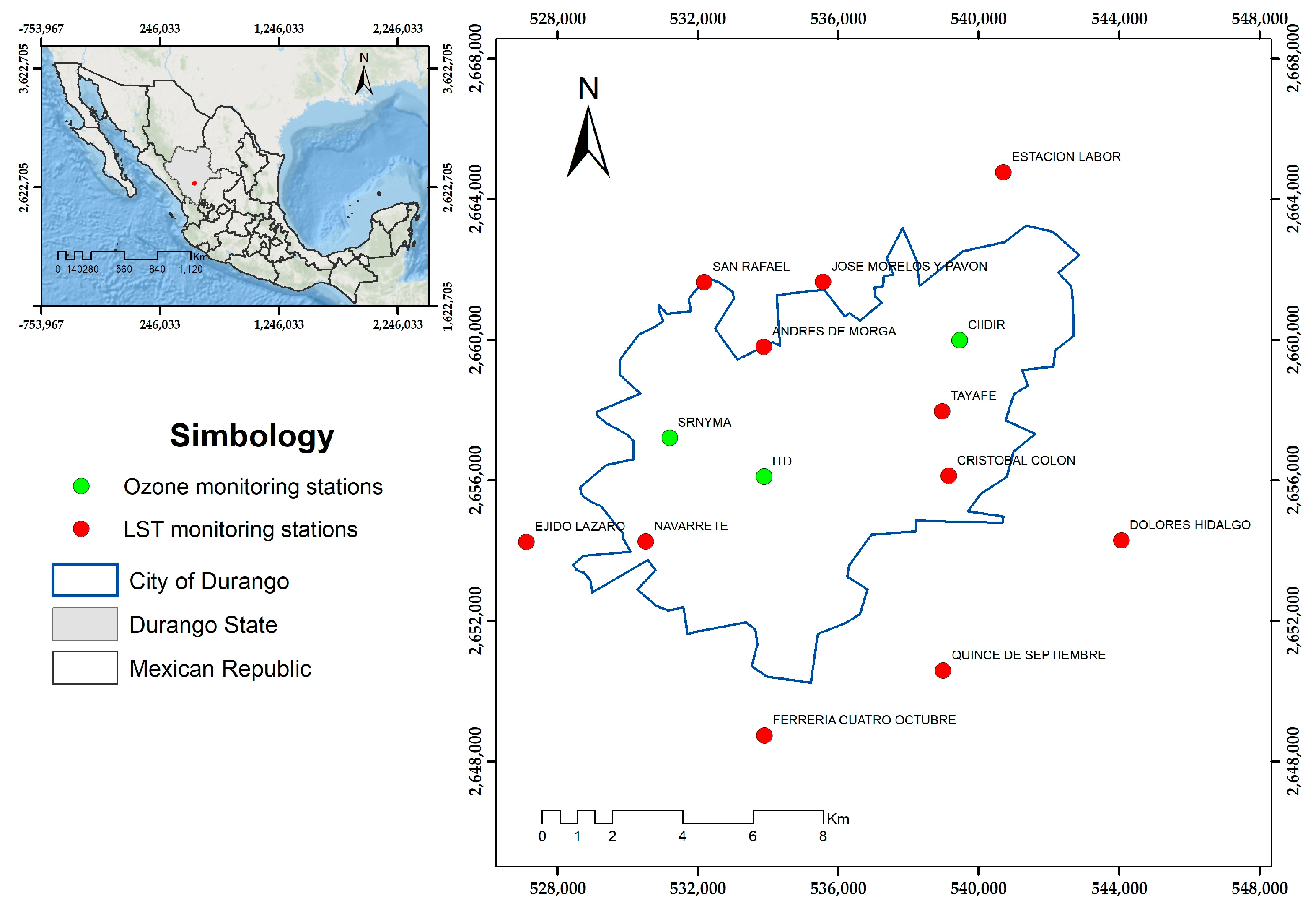
2.1. Study Area

The city of Durango is the capital of the State of Durango and is located between the coordinates 24°4′43.34″, −104°34′57.03″, 23°58′53.83″, −104°36′30.22″, with an altitude of 1890 m. The Figure 1 shows the study area, formed by the urban area of the city, and the 14 sampling points of which 11 were obtained by collecting from temperature-monitoring station data and the rest from three fixed monitoring stations established in the city, specifically located in Ministry of Natural Resources and Environment (SRNyMA), Durango Institute of Technology (ITD) and Interdisciplinary Research Center for Regional Integral Development Durango Unit (CIIDIR).

2.2. Data on Tropospheric Ozone Concentrations (O₃)

From the three fixed stations in the city of Durango (SRNyMA, ITD and CIIDIR), O₃ concentration data were obtained for each corresponding month of the year 2023. Monthly averages were calculated for both variables (12 data points corresponding to the 12 months of 2023). The information concerning 14 temperature sampling data was extracted from the worldwide meteorological and air quality data visualization and has a HRRR (High-Resolution Rapid Refresh) model. Variables such as temperature and ozone were also extracted in this application. It is a real-time model with a resolution of 3 km (km), and is updated every hour, with atmospheric correction from NOAA (National Oceanic & Atmospheric Administration).

2.3. Land Surface Temperature (LST) from Landsat 8 Satellite

The LST data from year 2023 were obtained from a free code generated by Sofia Ermida in 2020 [38], this code is open to use Google Earth Engine and operates with Landsat 8 imagery. Landsat 8 solar radiation data are generated using the Land Surface Reflectance Code (LaSRC) algorithm, where the atmospheric correction is performed using a radiative transfer model, auxiliary atmospheric data from MODIS, and makes use of the coastal aerosol band for aerosol inversion tests. To obtain complete spatial information in the surface temperature study area, the LST image for each month of the year 2023 was downloaded. Once the LST image was obtained for each month, the LST value for each of the stations was extracted to correlate the O₃ concentrations with the LST. This process of extracting values was performed using the “ex-tract” function, which allows for the extraction of values from a raster with a spatial object in RStudio software (version 2023.03.0) [40].

2.4. Statistical Analysis

In order to evaluate the linear association between O₃ and LST, a Pearson correlation analysis (r) was used for each time period and then a linear regression analysis was applied to predict ozone concentrations in the city, where the dependent variable corresponds to ozone concentrations and the independent variable is temperature. The simple linear regression model corresponds to the following equation

Y = β₀ + β₁ X + ε.

where “Y” is the O₃ concentration, “B₀” is the cut-off height of the Y-coordinate axis, “B₁” is the increment in Y according to X, and “X” is the LST and “ε “ is the error.

Goodness-of-fit coefficients such as the Coefficient of Determination (R²) and the Root Mean Square Error (RMSE) were calculated to evaluate the model’s ability to fit. Once the model was evaluated, the spatial O₃ concentration map was generated. These analyses were performed with RStudio software [40].

$${\mathrm{R}}^2=1-\left[{\displaystyle \frac{{\sum }_{i=1}^n(y_i-{\widehat{y}}_i{)}^2}{{\sum }_{i=1}^n(y_i-{\overline{y}}_i{)}^2}}\right]$$

$$\mathrm{RMSE}=\sqrt{{\displaystyle \frac{{\displaystyle \sum _{i=1}^n{(y_i-{\widehat{y}}_i)}^2}}{n-p}}}$$

where $y_i$ = observed parameter, ${\widehat{y}}_i$ = estimated parameter, ${\overline{y}}_i$ = mean of parameter, $n$ = number of total observations, and $p$ = number of model parameters.

3. Results

Figure 2 shows the behavior of O₃ concentrations and SST behavior in each month of 2023. High O₃ concentrations were identified in February and June, and the lowest in October. Similarly, the highest temperature was recorded in June and the lowest in November. It can be observed that in summer (May, June, and July), there were high O₃ concentrations along with an increase in temperature, and in winter (December, January, and February), as temperatures decreased, there was an increase in ozone.

Table 1. Simple linear regression parameters.

Month	Model	r	Standard Residual Error	p-Value	R2	RMSE (ppm)
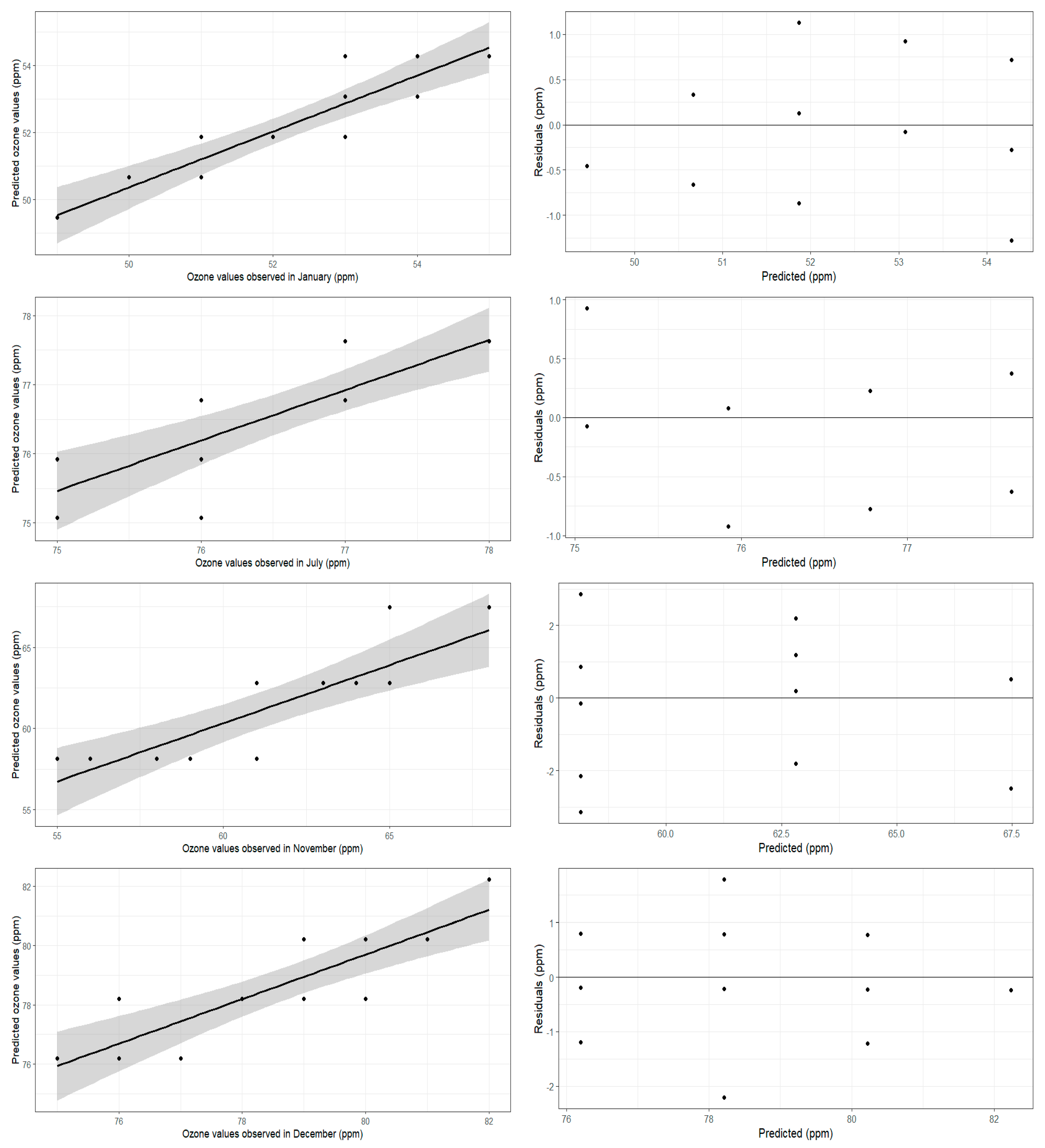
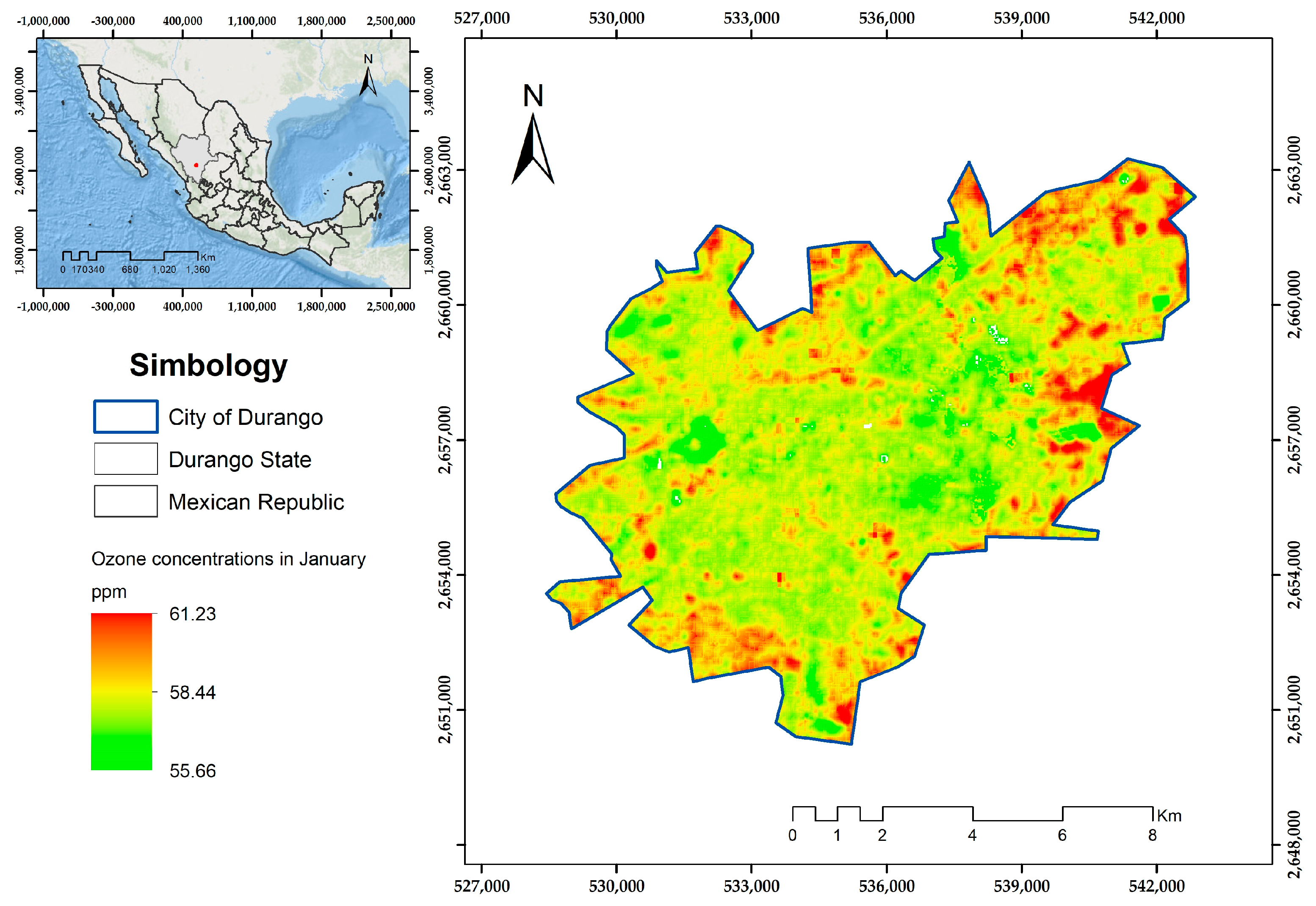
January	y = 24.14 + 1.20 (LST)	0.91	0.7099	0.0005	0.83	0.65
February	y = 113.41 − 0.27 (LST)	−0.28	0.6111	0.3253	0.08	0.56
March	y = 215.67 − 4.90 (LST)	−0.51	7.5021	0.0611	0.26	6.94
April	y = 89.84 + 0.13 (LST)	0.28	0.4681	0.3286	0.08	0.43
May	y = 141.74 − 1.58 (LST)	−0.33	3.9141	0.2435	0.11	3.62
June	y = 160.15 − 1.51 (LST)	−0.59	1.796	0.0246	0.35	1.66
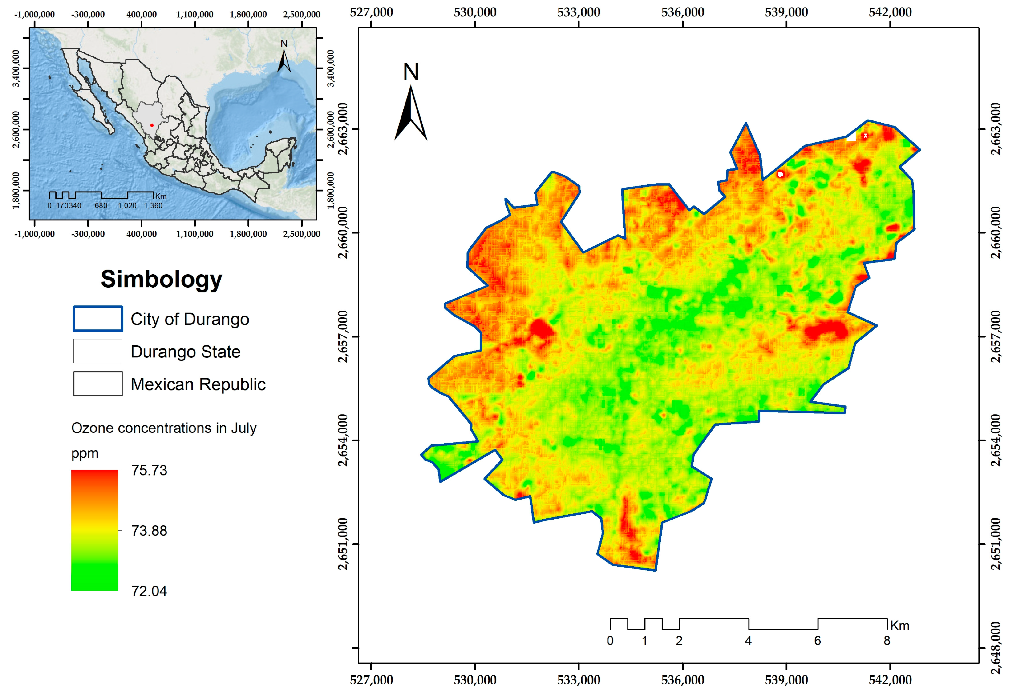
July	y = 101.47 − 0.85 (LST)	−0.85	0.5794	0.0001	0.73	0.53
August	y = 67.10 − 0.13 (LST)	−0.31	0.4691	0.2754	0.09	0.43
September	y = 81.05 − 0.18 (LST)	−0.27	1.092	0.3505	0.07	1.02
October	y = 61.47 − 0.26 (LST)	−0.36	0.5928	0.2021	0.14	0.54
November	y = 160.95 − 4.67 (LST)	−0.85	2.276	0.0001	0.72	2.18
December	y = 122.50 − 2.01 (LST)	−0.87	1.094	0.0005	0.75	1.02

Where y = dependent variable (ozone concentration = O₃); x = independent variable (LST).

shows the results of the correlation analysis between O₃ concentration and SST recorded by the sensor, showing a positive linear association in January (r = 0.91). It can be observed that SST had a negative and significant correlation in the months of July, November, and December (r = −0.85, −0.85 and −0.87, respectively). On the other hand, the regression analysis showed an R² range of 0.07 to 0.83 for the different months of the year. The model that best predicted O₃ concentrations through the independent variable LST was for January, with an R² = 0.83 (RMSE = 0.65 parts per million (ppm), indicating that the regression model explained 83% of the total variance (Table 1). In addition, in Figure 3, the observed versus predicted values from the best prediction models are presented, as well as the residual plot for each model by month.

Once the model was determined, the raster calculator was applied to generate the spatial distribution of O₃ concentrations in parts per million (ppm) in the city during January, July, November, and December (Figure 4, Figure 5, Figure 6 and Figure 7). Wang et al. 2003 found that the O₃ values simulated using neural networks during summer and winter months were better than those in spring and autumn in the urban area of Honk Kong, with three monitoring stations at Tsuen Wan, Kwai Chung, and Kwun Tong [41].

Periods with higher O₃ concentrations have mainly been associated with anticyclonic weather systems, in which the sun, low wind speed, and temperature changes allow for the formation of a tropospheric layer that inhibits convective mixing; therefore, ozone tends to be more persistent in the winter months [42].

4. Discussion

The correlation analysis showed a positive linear correlation between O₃ concentrations and LST derived from remote sensors in January (r = 0.91). It can be observed that LST presented a negative and significant correlation in the months of July, November, and December (r = −0.85, −0.85, and −0.87, respectively). The relationship of O₃ with temperature is linear in the multi-year analysis. In studies such as [29], studied over a range of 21 years, the relationship was always linear, corresponding to what we observed in this study (Figure 2). This relationship is determined by the photochemical origin of O₃: The higher the solar radiation, the higher the O₃ concentration. This process has been demonstrated in some studies, which explain that the highest O₃ generation usually appears at the time of day with the higher temperature record [18,27,28]. In this study, the correlation coefficients were based on a monthly analysis, but an hourly analysis throughout the day would yield a similar result to the study conducted in the metropolitan area of Mexico City by [33], where the behavior of the correlation between O₃ and temperature decreased gradually in the morning and at night and the maximum values were presented between the hours of 15:00 and 17:00 h. This result was similar to that reported by [34], who reported a positive correlation (r = 0.89) between O₃ and temperature for two zones of China during the month of May, considered the hottest month in the country [11,17]. On the other hand, ref. [34] reported a lower correlation (r = 0.57), in the June to September season in India.

Given these relationships that were presented between O₃ and LST, the prediction of O₃ showed that the best prediction model was from January (R² = 0.83). This result was similar to that found by Pavón-Domínguez [43], who concluded that they used a multiple linear regression analysis (R² = 0.89) with meteorological variables to estimate O₃ concentration in different urban areas of Seville, Spain. On the other hand, in the study by Navarro [37], whose objective was to analyze the most important meteorological variables in the variation of surface ozone concentration in Biella, Italy, lower values were observed in the fit coefficients in the linear models used (R² = 0.40). In the study of Otero [17], in a study conducted in Germany, they used generalized additive models in two 10-year periods (from 1999 to 2008 and from 2009 to 2018), obtaining minimum values of coefficients of determination (R²) of 0.10 and maximum values of 0.46 in the first period and values between 0.07 and 0.43 in the second period, indicating that the lowest values correspond to those recorded in the rural area and the high values to the urban area.

The R² values found in the present study compared to the values found in other studies may be attributed to monthly media concentrations of pollutant precursors present in the study area, as well as to other factors such as humidity or wind speed. On the northwest side of the city, a wave of high O₃ concentrations is perceived. According to previous research [39], the wind in this season usually comes from the southwest direction, which contributes to ozone concentrations traveling in this direction. According to the above, the variation in O₃ concentration varies with the different seasons of the year, since atmospheric conditions favor the accumulation of this pollutant at ground level; however, other factors such as the absence of wind and rain can contribute to O₃ concentrations [15,44]. In addition, O₃ concentrations also vary with the presence of vegetation in urban areas. In the study area of the present research, there is a public park, and in this area, there were lower O₃ concentrations in the same hot season. This is due to the fact that vegetation contributes to the photochemical generation of O₃, which is induced by natural emissions of volatile organic compounds (VOCs) from the oxidation of nitrogen in the existing vegetation, thus becoming areas of influence on O₃ concentration [45].

These are typical conditions in the city of Durango for this season, which historically is part of the hottest and driest in the state. Other factors [46,47,48,49], such as increased air turbulence, photochemical activity and increased concentration of precursors such as NOx and Sox [50,51], should be analyzed with respect to photochemical smog formation, which should be further investigated in future work [52,53,54]. This is because the photochemical cycle of O₃ presented a behavior characteristic of urban areas, with minimum values in the early morning hours and an increase after 8:00 am, with maximum values at noon. It should also be considered that photochemical activity is higher in the summer period [55], so this study is limited to one month of this period. This study was initiated by calculating the O₃ tendency and LST. Due to the randomness of the atmospheric levels of pollutants, an attempt was made to explain their behavior by means of regression models to determine the possible correlation between LST and ozone. The results of the present study showed that the maximum O₃ monthly concentrations did not exceed the national air quality standard on the days evaluated as in the case of other studies [24,27]. This highlights the need for an environmental monitoring program to control emissions in the areas most vulnerable to the effects of this type of pollutants in urban areas, where tropospheric O₃ concentrations are increasing due to the gradual increase in temperature due to climate change [56,57]. Mexico, due to its geographical location (northern hemisphere), receives high rates of solar irradiance, an average greater than 4.6 kWh m⁻² day⁻¹, comparable to desert regions such as the Sahara Desert in Africa [58], which is the reason for the importance of this study, to predict O₃ concentrations that are generated in the city of Durango, México, corresponding to an area of high solar radiation analyzed by LST.

5. Conclusions

The goal of this study was to predict tropospheric O₃ concentrations from temperature data in the urban area of the city of Durango. Land surface temperature (LST) allowed for predicting O₃ concentrations in the urban area of the city of Durango. The highest correlation between O₃ and temperature was found in January. The model that best predicted ozone concentrations as a function of temperatures at different times of the day explained 91% of the total ozone variance. The present study shows the usefulness of satellite products such as LTS; however, the main limitation is the number of weather- and pollutant-monitoring stations in the urban area, so an increase in the number of stations in the areas with the highest incidence of temperature in the city should be prioritized. As shown in the present study, in order to establish mobile monitoring stations to improve the suitability of the model to predict the spatial distribution of ozone, even considering other variables such as wind speed, solar radiation, UV rays, and biogenic organic compounds that may be derived from the existing vegetation, an increase in the number of stations should be prioritized.

References

- World Health Organization. Ambient Air Quality Database WHO 2023. Available online: https://www.who.int/publications/m/item/who-ambient-air-quality-database-(update-2023) (accessed on 19 May 2023).
- Brunekreef, B.; Holgate, S.T. Air pollution and health. Lancet 2002, 360, 1233–1242. [Google Scholar] [CrossRef] [PubMed]
- Atkinson, R. Atmospheric chemistry of VOCs and NOx. Atmos. Environ. 2000, 34, 2063–2101. [Google Scholar] [CrossRef]
- Butler, T.; Lupascu, A.; Nalam, A. Attribution of ground-level ozone to anthropogenic and natural sources of nitrogen oxides and reactive carbon in a global chemical transport model. Atmos. Chem. Phys. 2020, 20, 10707–10731. [Google Scholar] [CrossRef]
- Galloway, J.N.; Townsend, A.R.; Erisman, J.W.; Bekunda, M.; Cai, Z.; Freney, J.R.; Martinelli, L.A.; Seitzinger, S.P.; Sutton, M.A. Transformation of the nitrogen cycle: Recent trends, questions, and potential solutions. Science 2008, 320, 889–892. [Google Scholar] [CrossRef] [PubMed]
- Monks, P.S.; Archibald, A.; Colette, A.; Cooper, O.; Coyle, M.; Derwent, R.; Fowler, D.; Granier, C.; Law, K.S.; Mills, G. Tropospheric ozone and its precursors from the urban to the global scale from air quality to short-lived climate forcer. Atmos. Chem. Phys. 2015, 15, 8889–8973. [Google Scholar] [CrossRef]
- Di, Q.; Rowland, S.; Koutrakis, P.; Schwartz, J. A hybrid model for spatially and temporally resolved ozone exposures in the continental United States. J. Air Waste Manag. Assoc. 2017, 67, 39–52. [Google Scholar] [CrossRef]
- U.S. Environmental Protection Agency. Greenhouse Gas Inventory Data Explorer. 2023. Available online: https://cfpub.epa.gov/ghgdata/inventoryexplorer/#allsectors/allsectors/allgas/gas/current (accessed on 19 May 2023).
- Lu, X.; Ye, X.; Zhou, M.; Zhao, Y.; Weng, H.; Kong, H.; Li, K.; Gao, M.; Zheng, B.; Lin, J. The underappreciated role of agricultural soil nitrogen oxide emissions in ozone pollution regulation in North China. Nat. Commun. 2021, 12, 5021. [Google Scholar] [CrossRef]
- Zhan, Y.; Luo, Y.; Deng, X.; Grieneisen, M.L.; Zhang, M.; Di, B. Spatiotemporal prediction of daily ambient ozone levels across China using random forest for human exposure assessment. Environ. Pollut. 2018, 233, 464–473. [Google Scholar] [CrossRef]
- Han, H.; Liu, J.; Shu, L.; Wang, T.; Yuan, H. Local and synoptic meteorological influences on daily variability in summertime surface ozone in eastern China. Atmos. Chem. Phys. 2020, 20, 203–222. [Google Scholar] [CrossRef]
- Roelofs, G.J.; Lelieveld, J.; van Dorland, R. A three-dimensional chemistry/general circulation model simulation of anthropogenically derived ozone in the troposphere and its radiative climate forcing. Geophys. Res. Atmos. 1997, 102, 23389–23401. [Google Scholar] [CrossRef]
- Echávez, K.; Pastran, Y.; Polo, Á. Estimación del CO2 emitido y capturado en la sede sabanas y el campus deportivo de la universidad popular del cesar. Rev. Ambient. Agua Aire Y Suelo 2015, 6. [Google Scholar] [CrossRef]
- Zhang, Y.; Cooper, O.R.; Gaudel, A.; Thompson, A.M.; Nédélec, P.; Ogino, S.-Y.; West, J.J. Tropospheric ozone change from 1980 to 2010 dominated by equatorward redistribution of emissions. Nat. Geosci. 2016, 9, 875–879. [Google Scholar] [CrossRef] [PubMed]
- Gong, C.; Liao, H. A typical weather pattern for ozone pollution events in North China. Atmos. Chem. Phys. 2019, 19, 13725–13740. [Google Scholar] [CrossRef]
- Jumin, E.; Zaini, N.; Ahmed, A.N.; Abdullah, S.; Ismail, M.; Sherif, M.; Sefelnasr, A.; El-Shafie, A. Machine learning versus linear regression modelling approach for accurate ozone concentrations prediction. Eng. Appl. Comput. Fluid Mech. 2020, 14, 713–725. [Google Scholar] [CrossRef]
- Otero, N.; Sillmann, J.; Mar, K.A.; Rust, H.W.; Solberg, S.; Andersson, C.; Engardt, M.; Bergström, R.; Bessagnet, B.; Colette, A. A multi-model comparison of meteorological drivers of surface ozone over Europe. Atmos. Chem. Phys. 2018, 18, 12269–12288. [Google Scholar] [CrossRef]
- Beristain-Montiel, E.; Gavilán-García, A.; Maldonado-Cabrera, S.C. Were biogenic volatile organic compounds mainly responsible for ozone pollution during the COVID-19 lockdown In Mexico City? J. Mex. Chem. Soc. 2023, 67, 12–23. [Google Scholar] [CrossRef]
- Emery, X. Geoestadística; Universidad de Chile: Santiago, Chile, 2013. [Google Scholar]
- Joseph, J.; Sharif, H.O.; Sunil, T.; Alamgir, H. Application of validation data for assessing spatial interpolation methods for 8-h ozone or other sparsely monitored constituents. Environ. Pollut. 2013, 178, 411–418. [Google Scholar] [CrossRef]
- Xu, J.; Zhang, Z.; Rao, L.; Wang, Y.; Letu, H.; Shi, C.; Tana, G.; Wang, W.; Zhu, S.; Liu, S.; et al. Remote sensing of tropospheric ozone from space: Progress and challenges. J. Remote Sens. 2024, 4, 0178. [Google Scholar] [CrossRef]
- Mettig, M.; Landgraf, J.; Hasekamp, O.P.; Brown, S.S.; Zuraski, K.; Chace, W.; Womack, C.C.; Peischl, J.; Hair, J.; Shingler, T.; et al. The Small Mobile Ozone Lidar (SMOL): Instrument description and first field measurements. Atmos. Meas. Tech. 2021, 18, 405–417. [Google Scholar] [CrossRef]
- Wang, S.; Huo, Y.; Mu, X.; Jiang, P.; Xun, S.; He, B.; Wu, W.; Liu, L.; Wang, Y. A High-Performance Convolutional Neural Network for Ground-Level Ozone Estimation in Eastern China. Remote Sens. 2022, 14, 16. [Google Scholar] [CrossRef]
- Zhao, L.; Zhai, Y.; Wang, X. Evaluation of satellite-based measurements of tropospheric ozone for air quality management: A review. Environ. Sci. Technol. 2021, 55, 6693–6705. [Google Scholar]
- Buele, M.; Alexander, E. Utilización de Información Satelital Para Estimar la Calidad del Aire a Nivel de Superficie Evaluación de Datos Satelitales de Ozono Troposférico en Contraste con la Información de Superficie de la Red Metropolitana de Monitoreo de Quito; Escuela Politecnica Nacional: Quito, Ecuador, 2024. [Google Scholar]
- Zhao, S.; Yang, X.; Li, Z.; Wang, Z.; Zhang, Y.; Wang, Y.; Zhou, C.; Ma, P. Advances of ozone satellite remote sensing in 60 years. Natl. Remote Sens. Bull. 2022, 26, 817–833. [Google Scholar] [CrossRef]
- Moreno, L.V.; Perilla, J.K. Análisis de la Calidad del Aire en Villa de Leyva-Boyacá a Partir de Mediciones de Dióxido de Azufre Generadas por el Satélite Sentinel 5P; Universidad Distrital Francisco José de Caldas: Bogotá, Colombia, 2023. [Google Scholar]
- Chu, Y.Y.; Yao, J.; Qiao, D.W.; Zhang, Z.Y.; Zhong, C.Y.; Tang, L.J. Three-hourly PM2.5 and O3 concentrations prediction based on time series decomposition and LSTM model with attention mechanism. Atmos. Pollut. Res. 2023, 14, 101879. [Google Scholar] [CrossRef]
- Rezaei, R.; Naderalvojoud, B.; Güllü, G. A Comparative Study of Deep Learning Models on Tropospheric Ozone Forecasting Using Feature Engineering Approach. Atmosphere 2023, 14, 239. [Google Scholar] [CrossRef]
- Cheng, M.; Fang, F.; Navon, I.M.; Zheng, J.; Zhu, J.; Pain, C. Assessing uncertainty and heterogeneity in machine learning-based spatiotemporal ozone prediction in Beijing-Tianjin-Hebei region in China. Sci. Total Environ. 2023, 881, 163146. [Google Scholar] [CrossRef]
- Ghosh, A.; Manna, S. Monthly and annual oscillation of methane and ozone in eastern India using Sentinel-5P TROPOMI: Assessment and validation. Environ. Sci. Pollut. Res. 2025, 32, 208–225. [Google Scholar] [CrossRef]
- Chipa, S. Análisis de Contaminantes del aire Atmosférico a Través de Imágenes Sentinel 5P de la Región de Apurímac, Perú Periodo 2018–2021 Escuela de Posgrado Newman. 2023. Available online: https://repositorio.epnewman.edu.pe/handle/20.500.12892/716 (accessed on 16 February 2024).
- García Santos, D. Estimación de Calidad del aire en Superficie a Partir de Medidas Satelitales (Projecte Final de Màster Oficial); UPC, Escola Politècnica Superior d’Enginyeria de Manresa, Departament d'Enginyeria Minera, Industrial i TIC: Barcelona, Spain, 2021; Available online: http://hdl.handle.net/2117/354974 (accessed on 16 February 2024).
- Song, H.; Zhao, W.; Yang, X.; Hou, W.; Chen, L.; Ma, P. Ozone Sensitivity Analysis and Ozone Formation Regimes Division in the Beijing–Tianjin–Hebei Region Based on Satellite Remote Sensing Data. Atmosphere 2023, 14, 1637. [Google Scholar] [CrossRef]
- Mejía, D.; Faican, G.; Zalakeviciute, R.; Matovelle, C.; Bonilla, S.; Sobrino, J.A. Spatio-temporal evaluation of air pollution using ground-based and satellite data during COVID-19 in Ecuador. Heliyon 2024, 10, e28152. [Google Scholar]
- David, M.; Ibrahim, M.H.; Idrus, S.M.; Azmi, A.I.; Ngajikin, N.H.; En Marcus, T.C.; Yaacob, M.; Salim, M.R.; Aziz, A.A. Progress in ozone sensors performance: A review. J. Teknol. 2015, 73, 23–29. [Google Scholar] [CrossRef]
- Kerr, Y.H.; Lagouarde, J.P.; Nerry, F.; Ottlé, C. Land Surface Temperature Retrieval Techniques and Applications. Therm. Remote Sensing in Land Surface Processes; CRC Press: Boca Raton, FL, USA, 2004; pp. 33–109. [Google Scholar]
- Ermida, S.L.; Soares, P.; Mantas, V.; Göttsche, F.-M.; Trigo, I.F. Google Earth Engine Open-Source Code for Land Surface Temperature Estimation from the Landsat Series. Remote Sens. 2020, 12, 1471. [Google Scholar] [CrossRef]
- Loera-Sánchez, J.M.; Ramírez-Aldaba, H.; Meléndez Soto, A.; García-Montiel, E.; González-Laredo, R. Aplicaciones geoestadísticas para la evaluación de la contaminación por ozono en la ciudad de Durango, México. Nova Sci. 2021, 13. [Google Scholar] [CrossRef]
- R Core Team. R: A Language and Environment for Statistical Computing; R Foundation for Statistical Computing: Vienna, Austria, 2020; Available online: https://www.R-project.org/ (accessed on 9 April 2021).
- Wang, W.; Lu, W.; Wang, X.; Leung, A.Y. Prediction of maximum daily ozone level using combined neural network and statistical characteristics. Environ. Int. 2003, 29, 555–562. [Google Scholar] [CrossRef] [PubMed]
- Steinberger, E.H.; Ganor, E. High ozone concentrations at night in Jerusalem and Tel-Aviv. Atmos. Environ. 1980, 14, 221–225. [Google Scholar] [CrossRef]
- Pavón-Domínguez, P.; Jiménez-Hornero, F.; De Rave, E.G. Proposal for estimating ground level ozone concentrations at urban areas based on multivariate statistical methods. Atmos. Environ. 2014, 90, 59–70. [Google Scholar] [CrossRef]
- Navarro, C.M.; García, C.O. Impacto de la Meteorología en la Concentración de Ozono Troposférico; Universidad Complutense de Madrid: Madrid, Spain. Available online: https://cmougan.github.io/CV/files/tfg.pdf (accessed on 16 February 2024).
- Cano Baudino, Y.N.; Morales Mariño, J.A.; Sánchez Castillo, L.J.; Colina Rincón, M.N.; Torres Puente, J.C. Evaluación de los niveles de ozono en la Ciudad de Maracaibo, Estado Zulia, Venezuela. Rev. Int. Contam. Ambiental. 2016, 32, 25–34. [Google Scholar]
- Malley, C.S.; Henze, D.K.; Kuylenstierna, J.C.; Vallack, H.W.; Davila, Y.; Anenberg, S.C.; Turner, M.C.; Ashmore, M.R. Updated global estimates of respiratory mortality in adults ≥30 years of age attributable to long-term ozone exposure. Environ. Health Perspect. 2017, 125, 087021. [Google Scholar] [CrossRef]
- Bloomer, B.J.; Stehr, J.W.; Piety, C.A.; Salawitch, R.J.; Dickerson, R.R. Observed relationships of ozone air pollution with temperature and emissions. Geophys. Res. Lett. 2009, 36. [Google Scholar] [CrossRef]
- Bravo, J.L.; Nava, M.M.; Muhlia, A. Relaciones entre la magnitud del valor máximo de ozono, la radiación solar y la temperatura ambiente en la Zona Metropolitana de la Ciudad de México. Rev. Int. Contam. Ambiental. 2000, 16, 45–54. [Google Scholar]
- Gorai, A.; Biswal, S.; Mitra, G. Effects of meteorology on ground level ozone (GLO) concentrations and identifying the hot spots having significantly higher GLO concentration in a semi-urban area. Environ. Dev. Sustain. 2018, 20, 1461–1481. [Google Scholar] [CrossRef]
- Gunthe, S.; Beig, G.; Sahu, L. Study of relationship between daily maxima in ozone and temperature in an urban site in India. Curr. Sci. 2016, 110, 1994–1999. [Google Scholar] [CrossRef]
- Avino, P.; Manigrasso, M. Ten-year measurements of gaseous pollutants in urban air by an open-path analyzer. Atmos. Environ. 2008, 42, 4138–4148. [Google Scholar] [CrossRef]
- Jasaitis, D.; Vasiliauskienė, V.; Chadyšienė, R.; Pečiulienė, M. Surface ozone concentration and its relationship with UV radiation, meteorological parameters and radon on the eastern coast of the Baltic Sea. Atmosphere 2016, 7, 27. [Google Scholar] [CrossRef]
- Zoran, M.; Dida, M.R.; Savastru, R.; Savastru, D.; Dida, A.; Ionescu, O. Ground level ozone (O3) associated with radon (222Rn) and particulate matter (PM) concentrations in Bucharest metropolitan area and adverse health effects. J. Radio Anal. Nucl. Chem. 2014, 300, 729–746. [Google Scholar] [CrossRef]
- Pusede, S.; Gentner, D.; Wooldridge, P.; Browne, E.; Rollins, A.; Min, K.-E.; Russell, A.; Thomas, J.; Zhang, L.; Brune, W. On the temperature dependence of organic reactivity, nitrogen oxides, ozone production, and the impact of emission controls in San Joaquin Valley, California. Atmos. Chem. Phys. 2014, 14, 3373–3395. [Google Scholar] [CrossRef]
- Jing, P.; Lu, Z.; Xing, J.; Streets, D.G.; Tan, Q.; O’Brien, T.; Kamberos, J. Response of the summertime ground-level ozone trend in the Chicago area to emission controls and temperature changes, 2005–2013. Atmos. Environ. 2014, 99, 630–640. [Google Scholar] [CrossRef]
- Porter, W.C.; Heald, C.L. The mechanisms and meteorological drivers of the summertime ozone–temperature relationship. Atmos. Chem. Phys. 2019, 19, 13367–13381. [Google Scholar] [CrossRef]
- Schlink, U.; Dorling, S.; Pelikan, E.; Nunnari, G.; Cawley, G.; Junninen, H.; Greig, A.; Foxall, R.; Eben, K.; Chatterton, T. A rigorous inter-comparison of ground-level ozone predictions. Atmos. Environ. 2003, 37, S1352–S2310. [Google Scholar] [CrossRef]
- Orozco, S.; Rivero, M. Análisis de la Radiación Solar en Tres Ciudades de Coahuila y Durango. Rev. Cienc. Ing. Y Desarro. Tec Lerdo 2017, 3, 123–126. [Google Scholar]