Article

Mercury Intake Estimation in Adult Individuals from Trieste, Italy: Hair Mercury Assessment and Validation of a Newly Developed Food Frequency Questionnaire

1
Department of Cultural Heritage, University of Bologna, Via degli Ariani 1, 48121 Ravenna, Italy
2
Fano Marine Center, The Inter-Institute Center for Research on Marine Biodiversity, Resources and Biotechnologies (FMC), Viale Adriatico 1/N, 61032 Fano, Italy
3
Laboratory of Molecular Anthropology, Centre for Genome Biology, Department of Biological, Geological and Environmental Sciences, University of Bologna, Via Selmi 3, 40126 Bologna, Italy
4
Department of Prehistory, Archaeology and Ancient History, University of Valencia, Avenida de Blasco Ibañez 28, 46010 Valencia, Spain
5
Institute for Biological Resources and Marine Biotechnologies, National Research Council (IRBIM, CNR), Largo Fiera della Pesca 2, 60125 Ancona, Italy
6
Department of Analytical Chemistry, University of Valencia, Dr. Moliner 50, 46100 Burjassot, Spain
*
Author to whom correspondence should be addressed.
Pollutants 2023, 3(3), 320-336; https://doi.org/10.3390/pollutants3030022
Submission received: 28 April 2023 / Revised: 24 June 2023 / Accepted: 29 June 2023 / Published: 5 July 2023

Abstract

:
Seafood constitutes the primary source of exposure to the organic form of mercury in the general population, and the Trieste Gulf is considered a hotspot of mercury contamination. We used a newly developed quantitative food frequency questionnaire to obtain an estimation of the intake of mercury through seafood consumption in a sample of 32 individuals from Trieste. Then, we validated the results obtained from the questionnaire against those of the analysis of total mercury measured in the hair of the same individuals through Spearman rank correlation coefficients, Cohen’s weighted Kappa statistic, and a Bland–Altman plot. The Spearman rank correlation coefficient and Cohen’s weighted Kappa statistic were 0.76 and 0.69, respectively. In the Bland–Altman plot, 93.75% of the data points lay within the acceptability range. The plot revealed an ever-increasing overestimation of mercury intake by the questionnaires as the hair mercury increased. By applying a standardized filtering procedure to the results of the questionnaires, we obtained a Spearman rank correlation coefficient and Cohen’s weighted Kappa statistic of 0.69 and 0.57, respectively. In this Bland–Altman plot, 93.75% of the data points lay within the acceptability range. In this latter plot, the proportionality between the mean difference and the magnitude of the measurement was more subtle compared to that observed in the plot built upon the non-filtered questionnaires. This preliminary study shows the high accuracy of the reported questionnaire in the estimation of habitual mercury intake, similar to the one measured through the analysis of hair.

1. Introduction

Among the general population, seafood is the main source of exposure to the organic form of mercury, i.e., methylmercury (MeHg) [1,2], with large, long-lived, predatory fishes (e.g., Atlantic bluefin tuna, swordfish, and sharks) showing higher concentrations of this contaminant as an effect of biomagnification along the food chain [3] and MeHg uptake being a lifelong process of bioaccumulation [4].
MeHg is a well-established neurotoxicant, and exposure to MeHg is associated with nervous system damage in adults and impaired neurological development in infants and children [5], as well as with an increased risk of cardiovascular disease in adults [6].
Based on epidemiological evidence accumulated over the years, national and international agencies have set limits and given recommendations in order to protect citizens’ health. In 2001, the U.S. Environmental Protection Agency (US EPA) derived an oral reference dose (RfD) for MeHg—that is, the maximum oral dose that is likely to be without appreciable risk of deleterious effects during a lifetime—of 0.1 μg kg−1 day−1 [7,8]. Then, in 2012, the European Food Safety Authority (EFSA) Panel on Contaminants in the Food Chain (CONTAM) established a tolerable intake of 1.3 μg kg−1 body weight (b.w.) per week [9,10], corresponding to an apparent no-observed-effect level (NOEL) of ~11.5 mg kg−1 and ~46 μg L−1 in the hair and blood, respectively. This threshold value has been adopted for all classes of consumers, even though adults may be less sensitive to the adverse effects of MeHg [11].
Hair mercury level is frequently used as a biomarker of endogenous exposure to MeHg. Indeed, MeHg is permanently incorporated into the growing hair through diffusion from the blood, and the ratio between the total mercury (THg) in the hair and that in the blood is around 250:1 [12,13]. While blood can be used to document MeHg short-term exposure, hair provides an estimation of the long-term average exposure [12].
As several investigations have shown, hair THg level often depends on habitual seafood consumption [14,15,16,17,18,19,20,21,22,23,24,25,26]. In the study by Elhamri and colleagues on a Moroccan coastal community [15], the authors found a linear relationship between the log-transformed data on hair THg levels and the fish consumption frequency (FCF) in times per week. Moreover, they found that subjects with an FCF of three to five times per week showed greater hair THg levels (geometric mean = 5.30 μg g−1) compared to those of subjects with an FCF of one to two times per week (geometric mean = 1.04 μg g−1). Accordingly, when analyzing 237 adults from Naples (Italy), Díez and colleagues [16] found a strong positive correlation (rs = 0.536; p < 0.05) between the THg in hair and the fish consumption rate.
The Mediterranean Sea is generally considered a geological hot spot for Hg [11], as it is characterized by large deposits of mercury sulfur (HgS) that account for about 65% of the global mercury reserves [27], and the highest concentrations of Hg in Europe tend to be found in fish caught in the Mediterranean Sea [28]. Moreover, data have shown a more marked Hg bioavailability in the Tyrrhenian and the Adriatic coastal waters compared to the rest of the Mediterranean [29], and Hg levels higher than the legal limit have been discovered in seafood caught in both areas [4,30,31,32,33,34,35].
Considering all the above, and also the great amount of local seafood consumed by Mediterranean communities [11,20,36], it is not surprising that several studies revealed high hair THg levels in people from Mediterranean regions [23,37,38].
Among the methods aimed at estimating habitual seafood consumption [39,40] or the intake of specific nutrients [41,42] and/or contaminants [43], the food frequency questionnaire (FFQ) is one of the most used. The FFQ is a retrospective direct method for dietary assessment in that it collects information on the foods and beverages already consumed, assessing the frequency with which foods and/or food groups are eaten over a certain time period [44]. Whenever a new FFQ is developed, whether de novo or from pre-existing questionnaires, it should be validated in the investigated population on which the study is going to be conducted, which means that the results should be compared with those obtained applying at least another method [45], such as a dietary record [39,46], a 24 h recall [47,48], or the use of biomarkers [49,50].
Here, we used a newly developed quantitative FFQ—i.e., an FFQ that asks respondents’ usual portion size based on a specified measure—coupled with a database on Hg in Mediterranean seafood [51], to obtain an estimation of the intake of Hg through seafood consumption in a sample of 32 individuals from a coastal city in northern Italy, i.e., Trieste, which is considered a Hg contamination hotspot [52]. Then, we compared the results obtained from the questionnaire with those of the analysis of THg measured in the hair of the same individuals with the aim of (1) validating the questionnaire and (2) collecting preliminary data on Hg exposure among the population of Trieste.

2. Materials and Methods

2.1. Sampling Location

The Italian city of Trieste is located in the region of Friuli-Venezia Giulia, facing the northwestern part of the Adriatic Sea (Figure 1a). Trieste Gulf is considered a hotspot of Hg contamination, mostly due to the Hg input from the polluted Isonzo River (Figure 1b), which crosses the cinnabar-rich deposits of the Idrija mine [52].

2.2. FFQ Development and Administration

Following recommendations made in [44,45], we developed a quantitative FFQ consisting of close-ended questions on the habitual consumption of 52 aquatic species. These species were selected through the following procedure: we examined the Hg concentration data retrieved from the literature [4,30,31,33,34,35,52,53,54,55,56,57,58,59,60,61,62,63,64,65,66,67,68,69,70,71,72,73,74,75], coupled with a large database on Hg in Mediterranean biota [51], and calculated the average concentrations of Hg in the edible tissues of more than 350 Mediterranean aquatic species. Among these, we selected those species that are included in the ministerial decree of 22 September 2017 (n. 19105), listing species that are commercially relevant in Italy that show an average Hg concentration exceeding the maximum allowable level of Hg in seafood of 0.5 mg kg−1 set by EU [76] in their edible tissue, thus obtaining a list of 41 commercially relevant aquatic species contaminated by Hg in the Mediterranean Sea. Finally, we further expanded the above list by adding several species that are most consumed by the Italian population (ISMEA, 2011).
For each of the 52 species, the questionnaire assessed respondents’ habitual consumption frequency and portion size over a period spanning the previous six months before the interview. To ease species recognition, photos were shown to the participants, and species names in local dialects were provided. Apart from the questions on seafood consumption, the questionnaire included questions on other routes of exposition to Hg—i.e., breakage of Hg thermometers, occupation, dental amalgam fillings—smoking, and general state of health. The questionnaire was interviewer-administered through a voluntary response sampling carried out among the general population. The only two exclusion criteria pertain to the state of health of the participant—i.e., participants were required not to suffer from any specific illnesses and were asked to report their general state of health—and to the age of the participant—i.e., participants had to be 18 years of age and over. The sampling was approved by the bioethics committee of the University of Bologna.

2.3. Hg Intake Estimation from the FFQ

Once collected, the questionnaires were used to calculate the weekly Hg intake of the participants via the following formula:
Σ ( F   ( t i m e s   w e e k 1 ) × C   ( m g   k g 1 ) ) B W   ( k g ) ,
where F is the consumption frequency of each species in times week−1, C is the Hg concentration in the edible tissues of each species in mg kg−1, and BW is the body weight of the participant in kg.
After discovering, through comparison with hair THg levels, that the questionnaire tended to overestimate Hg intake in individuals consuming higher amounts of seafood, we applied a standardized filtering process to all 32 questionnaires; namely, for each participant, the estimation of Hg weekly intake was achieved using only those species that had been consumed at the two highest frequencies. For example, if a participant had consumed a given species twice a week, another species twice a month, and another one once a month, we excluded the last species from the calculation of the Hg weekly intake of that participant.

2.4. Hair Sampling and THg Measurement

Hairs of the participants were collected following the procedure recommended by the World Health Organization [12]. After a cleaning step involving rinsing the hair with 70% isopropyl alcohol, a bundle of hair approximately 0.75–1.0 cm in diameter was cut from the occipital region of each participant, using blunt-tipped, clean stainless steel. To make sure that an adequate amount (50 mg) of hair had been collected, samples were also weighed with a precision scale. Once cut, the hair bundle was wrapped close to the scalp end with a small Post-it note and held together with a plastic clip. Finally, the hair sample was placed in a marked paper envelope, which was in turn stored in a sealed plastic bag.
The measurement of THg concentration in hair samples was carried out using a Mercury Analyzer DMA-80 Milestone, which is a spectrophotometer based on the atomic absorption determination after the thermal decomposition of the samples.
The analysis process consists of introducing the sample into a small oven that can reach 650 °C. After the drying and incineration of the sample, the volatile compounds are carried by a flow of O2 to a catalyst, where the released mercury is reduced to Hg0, which is later retained in a small gold amalgam. The amalgam is heated to 900 °C, and the volatilized mercury passes through two measurement cells where it is quantified by detection using atomic absorption spectroscopy (AAS), with a detection limit of 0.5 μg kg−1 of Hg.
Once the amount of mercury expressed in ng is deduced, it is divided by the mass in grams of the sample, thus obtaining the result in concentration (μg kg−1).
1633c Trace Elements in Coal Fly Ash from NIST were used as certified reference material.
A solvent-free, easy, fast, and waste-free method was employed [77] using the EPA 7473 (SW-846) method. Each hair bundle was cut into pieces of ~1.5 cm in order to assess the monthly Hg intake, as each 1–1.5 cm segment of hair incorporates the Hg assimilated during the preceding month [78]. For each segment obtained, a quantity of ~10 mg of sample was weighted into a quartz cuvette. After that, 50 μL of ultrapure water was added to the sample in the cuvette, which was then introduced into the DMA-80. Samples were analyzed using the same temperature and time parameters as in [77], and for each 1.5 cm of a sample, we made two replicates, using their mean for statistical analyses.

2.5. Hg Intake Estimation from Hair THg

For each participant, to estimate their Hg intake from their hair THg level, we used the average of the THg concentrations measured in each ~1.5 cm segment of the hair sample. First, we derived the blood THg level using the above-mentioned ratio of 250:1 between the THg levels in the two matrices; hence, we obtained the estimate of the Hg dietary intake with the formula reported in [9]:
C   μ g   L 1 × b × V   ( L ) A × f × B W   ( k g )
where C is Hg concentration in blood in μg L−1, b is the elimination constant, which is equal to the ratio between ln (2) and Hg half-life in blood, which was assumed to be equal to 50 days as in [9], V is the blood volume, which was assumed to be equal to 5 L as has been assumed by WHO and US EPA [9], A is the gastrointestinal absorption factor (0.95), f is the fraction of absorbed dose distributed to blood, which was assumed to be equal to 0.05 as in [9], and BW is the body weight of the participant in kg.

2.6. Statistical Analysis

Statistical analyses were carried out using RStudio version 3.6.1.
After assessing the normality of data via Shapiro–Wilk normality test (R function: shapiro.test) and QQ-plots (R function: qqPlot), we used the Kruskal–Wallis rank sum test (R function: kruskal.test) to assess the statistical significance of the differences between the Hg intakes or hair THg concentrations in the two sexes, and we calculated Spearman rank correlation coefficients (R function: cor.test; method = “spearman”) to evaluate the association between the Hg intakes or hair THg concentrations and the age of participants.
To assess the validity of the FFQ, we compared the Hg intakes obtained with the two methods—i.e., the FFQ and the hair THg measurement—by calculating the Spearman rank correlation coefficients between the two and using Cohen’s weighted Kappa statistic (R function: cohen.kappa) which measures the extent to which the two methods assign the same participant to the same quintile. Finally, for the FFQ validation, we also used the Bland–Altman plot (R function: blandr.draw) [79,80], which is a graphical method that is recommended in conjunction with correlation coefficients when agreement between two quantitative methods has to be evaluated [45]. However, the correlation between results obtained with two different methods measuring the same quantity does not necessarily imply an agreement between the two methods [81]. Briefly, the Bland–Altman plot consists of a scatter plot, in which, the Y-axis shows the difference between each paired measurement (A and B)—i.e., the difference between the Hg intake estimated from the FFQ and that derived from the hair THg measurement—while the X-axis indicates the average of these measurements ((A + B)/2) [81]. When the difference between the two paired measurements is plotted against their mean, the two methods can be deemed in agreement if at least 95% of the data points lie within ±1.96s of the mean difference or within the non-parametric lower and upper limits of agreement (LOA) [82].

3. Results

3.1. Sample Characteristics

Information on participants is reported in Table 1 and Tables S1 and S2 of Supplementary File S1. The 32 participants were all adults and residents of Trieste and include 13 males and 19 females. The mean age was 35 among males (median = 32, SD = 10.90, and range: 21–55) and 48 among females (median = 51, SD = 11.63, and range: 20–65). Nine individuals, seven males and two females, were current smokers, and six participants, one male and five females, had dental amalgam fillings, while two female individuals were not able to provide this latter information.

3.2. Seafood Consumption

The average consumption of seafood products in our sample was 1.28 times a week, with minimal difference between males (1.32 times a week) and females (1.25 times a week) (Table 1). The species consumed in the largest quantity was the Gilthead seabream (Sparus aurata), with an average consumption rate of 161.82 g week−1, followed by common sole (Solea solea), with an average consumption rate of 79.62 g week−1, and squid (Loligo vulgaris), with an average consumption rate of 67.19 g week−1. The most frequently consumed species was Gilthead seabream (0.42 times week−1), followed by tuna (Thunnus spp.) (0.39 times week−1), and common sole (0.27 times week−1).

3.3. Exposure Assessment

3.3.1. FFQ

Including all the species consumed by participants, without any filtering procedure, we obtained a median Hg weekly intake of 2.62 μg kg−1 b.w. (mean = 4.08 μg kg−1 b.w., SD = 4.47, and range: 0.00–17.21 μg kg−1 b.w.), which is more than twice the EFSA maximum recommended intake. Among males, the median weekly intake was equal to 3.46 μg kg−1 b.w. (mean = 4.03 μg kg−1 b.w., SD = 3.13, and range: 0.52–9.55 μg kg−1 b.w.), while among females it was equal to 1.99 μg kg−1 b.w. (mean = 4.11 μg kg−1 b.w., SD = 5.28, and range: 0.00–17.64 μg kg−1 b.w.). Hg weekly intakes calculated from non-filtered FFQs were not normally distributed (Table S3 of Supplementary File S1). The difference between the Hg weekly intake of females and males was not statistically significant (Table S4 of Supplementary File S1), moreover, we found no statistically significant correlation between the inferred weekly intake and age, nor in the overall sample, nor in the two sexes separately (Table S5).
The first three species which contribute most to the habitual Hg intake in our sample were the European seabass (Dicentrarchus labrax), with an average intake of 31.92 μg week−1, Gilthead seabream, with an average intake of 30.85 μg week−1, and the Norway lobster (Nephrops norvegicus), with an average intake of 21.64 μg week−1.
After applying the above-described filtering procedure, i.e., including only those species that had been consumed at the two highest frequencies in the estimation of Hg intake of each participant, and assuming a negligible intake for the others, we obtained a median Hg weekly intake of 1.70 μg kg−1 b.w. (mean = 2.33 μg kg−1 b.w., SD = 2.13, and range: 0.00–8.00 μg kg−1 b.w.), which is still slightly higher than the EFSA maximum recommended intake. Among males, the median weekly intake after filtering of the questionnaires was equal to 2.12 μg kg−1 b.w. (mean = 1.98 μg kg−1 b.w., SD = 1.08, and range: 0.36–3.53 μg kg−1 b.w.), while among females it was equal to 1.23 μg kg−1 b.w. (mean = 2.57 μg kg−1 b.w., SD = 2.63, and range: 0.00–8.01 μg kg−1 b.w.). The Hg weekly intakes calculated from the filtered FFQs were not normally distributed (Table S3 of Supplementary File S1). Additionally, in this case, we found no statistically significant difference between the Hg weekly intake of males and females (Table S4 of Supplementary File S1). Moreover, we found no statistically significant correlation between the inferred weekly intake and age, nor in the overall sample, nor among female participants, while the inferred weekly intake and age showed a statistically significant negative correlation (τ = −0.5, p < 0.05) among male subjects (Table S5). After the filtering procedure, we found that Gilthead seabream was the species that contributed the most to the habitual intake of Hg in our sample, with an average intake of 26.03 μg week−1, followed by the European seabass, with an average intake of 23.13 μg week−1, and tuna, with an average intake of 18.73 μg week−1.

3.3.2. Hair Analysis
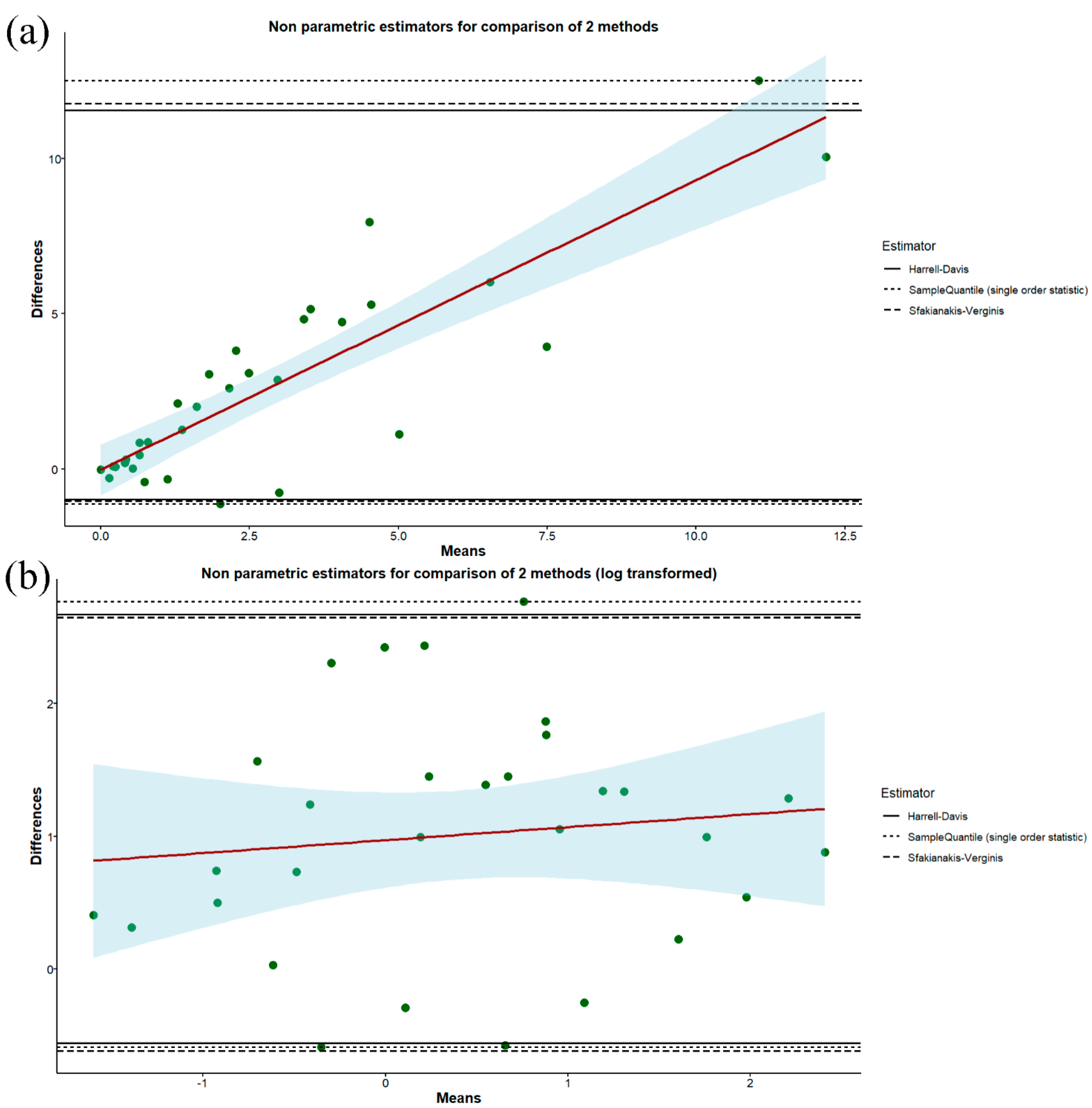
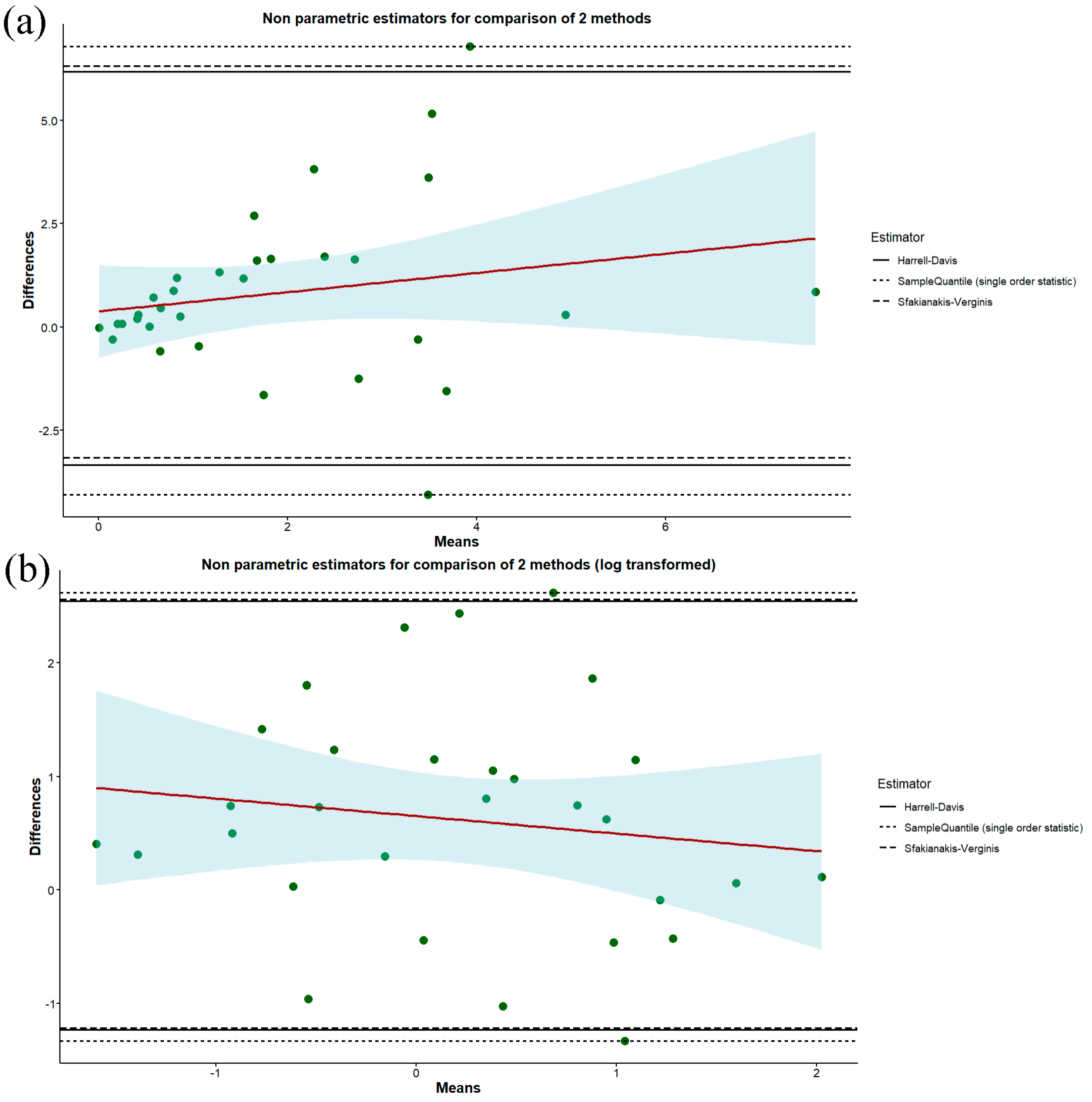
As can be seen from Figures S1 and S2 and Table S2 of Supplementary File S1, not all participants had long enough hairs to assess the Hg intake during the preceding six months, and for six male participants, only the first 1.5 cm of hair was available.
After averaging the THg concentrations measured in every ~1.5 cm segment of each participant’s hair, we found a median hair THg level in the analyzed sample of 1.08 mg kg−1 (mean = 2.02 mg kg−1, SD = 2.42, and range: 0.01–9.63 mg kg−1), which was well below the NOEL of ~11.5 mg kg−1 set by the EFSA. Concerning the difference between the two sexes, the results of the analysis of the hair are consistent with those of the FFQ, with male individuals being more exposed to Hg compared to female participants, and this difference was statistically significant (p < 0.05) (Table S4 of Supplementary File S1). Indeed, among males, the median hair THg level was equal to 2.07 mg kg−1 (mean = 2.91 mg kg−1, SD = 2.16, and range: 0.72–7.43 mg kg−1), while among females it was equal to 0.48 mg kg−1 (mean = 1.42 mg kg−1, SD = 0.48, and range: 0.02–9.63 mg kg−1). Consistently, with the results obtained from the FFQ analysis, we found no statistically significant correlation between the hair THg level and age, nor in the overall sample, nor the two sexes separately (Table S5). Moreover, we found no statistically significant correlation between the hair THg concentration and the number of amalgam fillings, even after controlling for the number of cigarettes smoked a day and for seafood consumption frequency. Conversely, we found a weak but statistically significant positive correlation between the hair THg concentration and the number of cigarettes smoked a day, but only after controlling for the effect of the number of amalgam fillings and for seafood consumption frequency (Table S6 of Supplementary File S1). However, as shown by the Kruska–Wallis rank sum test, there was no statistically significant difference between smokers’ and non-smokers’ hair THg concentration, nor between participants with and without amalgam fillings (Table S4 of Supplementary File S1). Moreover, most of the participants—i.e., 23 out of 32—were non-smokers, and only 6 participants had dental amalgam fillings, therefore, these results must be interpreted with caution.
The hair THg level was used to derive the Hg dietary intake of each participant using (2). The median Hg weekly intake derived from hair THg level was equal to 0.80 μg kg−1 b.w. (mean = 1.50 μg kg−1 b.w., SD = 1.80, and range: 0.01–7.15 μg kg−1 b.w.), which is lower than the EFSA maximum recommended intake and the values obtained from the FFQ, both before and after filtering. Among males, the median weekly intake was equal to 1.54 μg kg−1 b.w. (mean = 2.16 μg kg−1 b.w., SD= 1.61, and range: 0.53–5.52 μg kg−1 b.w.), while among females it was equal to 0.36 μg kg−1 b.w. (mean = 1.05 μg kg−1 b.w., SD = 1.82, and range: 0.01–7.15 μg kg−1 b.w.).

3.4. FFQ Validation

The Spearman rank correlation coefficient showed that the Hg weekly intakes derived from the non-filtered FFQs were positively correlated with those derived from hair THg concentrations (Table 2; Figure S3 of Supplementary File S1) and that this positive correlation is strong and statistically significant (R = 0.76, p < 0.05).
The weighted Kappa statistic was equal to 0.69, pointing to a moderate agreement between the two methods [83]. Then, we built the Bland–Altman plot upon the two series of data. In the case of a few participants, the FFQ and hair THg measurement returned intake values that were markedly more discordant than the other paired values. Accordingly, the Shapiro–Wilk normality test showed that the differences between each paired measurement were not normally distributed. As stated by Bland and Altman, when there are one or more extreme discrepancies between the method—i.e., the difference between one or more pair of measurements differs considerably from the others—a nonparametric approach may be preferable. Therefore, as suggested by Frey and colleagues [84], we used quantile estimation based on one and two-order statistics—i.e., Harrell–Davis quantiles, sample quantiles, and the Sfakianakis–Verginis quantiles estimator—to derive the non-parametric limits of agreement. The mean difference between the two methods was equal to 2.57. The resulting plot (Figure 2a) showed that 93.75% of the data points—i.e., 30 out of 32—lay within the acceptability range determined by the sample quantiles (lower LOA = −1.13, upper LOA = 12.51), by Harrell–Davis quantiles (lower LOA = −0.99, upper LOA = 11.55), and by Sfakianakis–Verginis quantiles estimator (lower LOA = −1.02, upper LOA = 11.76).
The Bland–Altman plot in Figure 2a also reveals an ever-increasing overestimation of Hg intakes by the FFQ as the hair THg level increases. In other words, the mean difference between the two methods was approximately proportional to the magnitude of the measurement, and this is made apparent by the substantial slope of the red line shown in the plot. Therefore, we tried to build the plot using the logarithms of the two data series, as suggested by Bland and Altman [79], after excluding two female participants for whom their weekly Hg intake from the FFQ was equal to zero. In this new plot (Figure 2b), 93.75% of the data points—i.e., 30 out of 32—lay within the acceptability range determined by the sample quantiles (lower LOA = −0.59, upper LOA = 2.77), while 90% of the data points—i.e., 27 out of 30—lay within the acceptability range determined by the Harrell–Davis quantiles (lower LOA = −0.56, upper LOA = 2.67), and 96.67% of the data points—i.e., 29 out of 30—lay within the acceptability range determined by the Sfakianakis–Verginis quantiles estimator (lower LOA = −0.62, upper LOA = 2.65). Additionally, in this case, the proportionality between the mean difference and the magnitude of the measurement persisted, even if at a lower level.
Given the bias that the non-filtered FFQ showed in the assessment of the Hg weekly intake, we filtered participants’ answers through several procedures, each time assessing the resulting improvement through the Bland–Altman plot. In this way, we found that the best results were obtained when only those species that had been consumed at the two highest frequencies were included in the calculation of the Hg weekly intake of each participant. Furthermore, in this case, the Spearman rank correlation coefficient showed that the Hg weekly intakes derived from the filtered FFQ were positively correlated with those derived from the hair THg concentrations (Table 2; Figure S4 of Supplementary File S1) and that this positive correlation is strong and statistically significant (R = 0.61, p < 0.05). The weighted Kappa statistic was equal to 0.57, pointing to a weak agreement between the two methods [83]. The Bland–Altman plot built upon the same filtered data (Figure 3a) showed that 93.75% of the data points—i.e., 30 out of 32—lay within the acceptability range determined by the sample quantiles (lower LOA = −4.06, upper LOA = 6.79), by the Harrell–Davis quantiles (lower LOA = −3.35, upper LOA = 6.18), and by the Sfakianakis–Verginis quantiles estimator (lower LOA = −3.16, upper LOA = 6.31).
The proportionality between the mean difference and the magnitude of the measurement was more subtle compared to that observed in the plot built upon the non-filtered FFQs. Then, we built the Bland–Altman plot using the log-transformed hair THg concentrations and Hg intakes from filtered FFQs. In this case (Figure 3b), 93.75% of the data points—i.e., 30 out of 32—lay within the acceptability range determined by the sample quantiles (lower LOA = −1.33, upper LOA = 2.62), by the Harrell–Davis quantiles (lower LOA = −1.23, upper LOA = 2.55), and by the Sfakianakis–Verginis quantiles estimator (lower LOA = −1.22, upper LOA = 2.56). In this latter plot, the mean difference between the two methods slightly decreased as the magnitude of the measurement increased.

4. Discussion

4.1. FFQ Reliability

It has been suggested that the correlation coefficients in validation studies should not be below 0.3–0.4 [39,45], and results derived from both the non-filtered and the filtered questionnaires developed in the present study meet this requirement.
Regarding the weighted Kappa statistic, in his original paper, Cohen suggested that values of Kappa ≤ 0 indicate no agreement, and interpreted values between 0.01 and 0.20 as none to slight, values between 0.21 and 0.40 as fair, values between 0.41 and 0.60 as moderate, values between 0.61 and 0.80 as substantial, and values between 0.81 and 1.00 as almost perfect agreement [85]. However, other authors have suggested that any Kappa below 0.60 should be interpreted as an indication of the inadequate agreement between the two methods, especially in a clinical context [83]. On the basis of such premises, we conclude that the FFQ developed in the present study, both before and after filtering, shows a moderate to a substantial agreement with the hair THg measurement.
A strong correlation does not imply an agreement between the two methods [80], and that is why correlation should be used alongside the Bland–Altman plot [45]. Results of the Bland–Altman plots with non-parametric LOAs showed that the filtered FFQ is more reliable in assessing the Hg weekly intake compared to the non-filtered version, as the latter tends to overestimate the Hg intake in individuals consuming higher amounts of seafood. However, it is important to note that the requirement for the validation—i.e., at least 95% of the data points lying within ±1.96s of the mean difference or the non-parametric lower and upper LOA—was met only in the case of the log-transformed data series from the non-filtered FFQs and hair THg concentration, using the Sfakianakis–Verginis quantiles as LOA. In most other cases, only 93.75% of the data points lay within the non-parametric range of acceptability, with the above percentage dropping to 90% in the case of the log-transformed data series from the non-filtered FFQs and hair THg concentration, and using the Harrell–Davis quantiles as LOA.
Overall, the results of the present study are promising and point to the fair efficacy of the newly developed FFQ in assessing habitual Hg intake.
As stated by Cade and colleagues in their review [45], for the Bland–Altman method, a sample size of at least 50 is desirable, while, for validation studies using correlation coefficients, this number rises to 100. Therefore, administering the FFQ to a larger sample may strengthen the validity assessment.
Another limitation of the present study is that we did not check the accuracy of the answers because each participant answered the questionnaire only once. Indeed, it is advisable to administer the questionnaire twice, in order to compare the answers given the first time with those given the second.
Finally, a potential source of error in the present investigation stems from the fact that we do not know the exact geographic origin of the seafood consumed by the participants. This may be a source for errors in the estimation of Hg intake via the FFQ, as seafood contamination also depends on local oceanographic factors and the vicinity of emission sources.

4.2. Hg Exposure

The FFQ, both before and after filtering, returned a median Hg weekly intake that was higher than the value derived from the hair THg measurement. In particular, the non-filtered FFQ returned a value (2.62 μg kg−1 b.w.) that is more than twice the EFSA maximum recommended intake of 1.3 μg kg−1 b.w. per week [9,10], and the filtered FFQ returned a value (1.70 μg kg−1 b.w.) that is only slightly higher than the same limit. On the other hand, the median Hg weekly intake derived from the hair THg measurement was equal to 0.80 μg kg−1 b.w., which is lower than EFSA’s maximum recommended intake.
The median hair THg concentration in the analyzed sample from Trieste is equal to 1.08 mg kg−1, which is well below the NOEL of ~11.5 mg kg−1 set by the EFSA. However, it is important to note that there is no consensus on the actual hair THg level above which health risk may occur, as several investigations have led to the establishment of threshold values ranging from 1, set by the US EPA [86], to 14 mg kg set by the Joint FAO/WHO Expert Committee on Food Additives (JECFA) [87]. In total, 16 out of the 32 participants in this study exhibited hair THg concentrations higher than 1 mg kg−1, and 6 participants exhibited concentrations higher than 3.75 mg kg−1, which is the concentration at which adverse health effects are possible according to the German Human Biomonitoring Commission [88], and only 1 female participant exhibited a THg concentration slightly greater than the EFSA NOEL of 11.5 mg kg−1 in one single ~1.5 cm segment of her hair, roughly corresponding to the period from February to March 2021.
The median hair THg concentration obtained in the present study is greater than that found by Basu and colleagues [23] for the populations of Africa (0.69 mg kg−1) and Europe (0.30 mg kg−1), for the populations living on the coast of the Atlantic (0.62 mg kg−1) and Arctic (0.74 mg kg−1) oceans, and those on the coast of the Mediterranean Sea (0.88 mg kg−1), while it is lower than that found in the same study for populations in the Americas (2.02 mg kg−1), eastern Mediterranean (1.68 mg kg−1), southeast Asia (3.10 mg kg−1) and western Pacific (1.40 mg kg−1), and for the coastal populations of the Pacific Ocean (1.75 mg kg−1) and fish consumers—i.e., non-Indigenous or non-Arctic groups who consume relatively high amounts of seafood—(3.04 mg kg−1).
The coastal town of Grado, in Friuli-Venezia Giulia, is less than 30 km from Trieste (Figure 1b) and is strongly impacted by Hg pollution due to maritime traffic, a local chlor-alkali plant, and the former Idrija mercury mine in Slovenia. An investigation carried out on 19 inhabitants of this town found a hair THg concentration ranging from 1.13 to 20.16 mg kg−1, the highest values being measured among fishermen, with a median value (3.90 mg kg−1) well above that found in the present study. On the other hand, in another study on the same geographic area [89], the authors found a mean hair THg concentration of 0.83 mg kg−1 among mothers of children with advanced fine motor skills, and of 1.24 mg kg−1 among mothers of children who showed normal or delayed skills. Both of these values are lower than the mean hair THg concentration exhibited by the sample analyzed in our investigation (2.02 mg kg−1), and, accordingly, the two groups of mothers in that study showed a fresh fish intake during pregnancy of 0.47 and 0.66 servings per week, respectively, while the 32 participants from Trieste showed a mean seafood intake of 1.28 servings per week.
Compared to our results, lower hair THg concentrations are also shown by the general population of several towns on the coast of Sicily (mean concentration = 0.23 mg kg−1, SD = 0.4) [21], by people living in Priolo, near the chlor-alkali plant of Augusta (Sicily), one of the largest in Europe (mean concentration = 1.37 mg kg−1, median concentration = 1.00 mg kg−1), and by the general population of Naples (mean concentration = 0.638 mg kg−1). On the contrary, higher THg concentrations were found in fishermen of several coastal towns of Sicily (mean concentration = 6.45 mg kg−1, SD = 7.03), in people from Augusta (mean concentration = 2.61 mg kg−1, median concentration = 1.90 mg kg−1), and in tuna consumers from Carloforte (Sardinia) (median concentration = 9.6 mg kg−1, range: 1.4–34.5 mg kg−1).
It is important to note that, due to its small size, the sample analyzed in the present study may not be representative of the entire population of Trieste.
Finally, it comes as no surprise the fact that, as revealed by the questionnaires, Gilthead seabream, European seabass, squid, and tuna are the species that contribute the most to the habitual Hg intake of the participants, since the first three species are among those that are the most consumed in Italy, and tuna is one of the most contaminated species.

5. Conclusions

To gain insights into the Hg exposure level among a Mediterranean community living in an area that is considered a contamination hotspot—i.e., the Trieste Gulf—we developed and validated a new FFQ and compared its results against those of the analysis of the total mercury measured in the hair of the same individuals. The reported newly developed questionnaire shows high accuracy in the estimation of habitual mercury intake, similar to the one measured through the analysis of the hair. Moreover, the questionnaire allowed us to obtain a first glimpse of the exposure to Hg from seafood among the population of Trieste.

Supplementary Materials

The following supporting information can be downloaded at: https://www.mdpi.com/article/10.3390/pollutants3030022/s1, Supplementary-File S1: Supplementary materials. Figure S1: Hair THg concentrations (Y-axis) in the first four ~1.5-cm segments of hair (X-axis) in female participants, starting from the nearest (1) to the farthest (4) from the scalp. Each line color corresponds to a participant, with bigger colored dots representing measurements. On top of the graph are shown the periods around which the detected Hg was ingested. The red transparent bar represents the evolution of the mean hair THg level. Figure S2: Hair THg concentrations (Y-axis) in the first four ~1.5-cm segments of hair (X-axis) in male participants, starting from the nearest (1) to the farthest (4) from the scalp. Each line color corresponds to a participant, with bigger colored dots representing measurements. On top of the graph are shown the periods around which the detected Hg was ingested. The red transparent bar represents the evolution of the mean hair THg level. Figure S3: Scatterplot for the weekly Hg intake from the hair THg concentration and non-filtered FFQ, with a regression line based on the Spearman rank correlation coefficient. Figure S4: Scatterplot for the weekly Hg intake from the hair THg concentration and filtered FFQ, with a regression line based on the Spearman rank correlation coefficient. Table S1: Information and results on each study participant. Reported hair THg was calculated by averaging the THg concentrations measured in every ~1.5 cm segment of hair and is expressed in mg kg−1, while intakes are in μg kg−1 body weight. Table S2: Hair THg concentrations (mg kg−1) in the first four ~1.5-cm segments of hair of each study participant. Table S3: Results of the Shapiro–Wilk normality test on several data series (first column). In bold are the p-values indicating a normal distribution (p-value > 0.05). Table S4: Results of the Kruskal–Wallis rank sum test aiming to assess the statistical significance of differences between the Hg intakes or hair THg concentrations of the two sexes. Table S5: Spearman rank correlation coefficients between several data series and the age of participants. Supplementary-File S2: original FFQ in Italian. Supplementary-File S3: FFQ translated in English.

Author Contributions

Conceptualization, A.D.G., G.G., C.G., M.L.C. and D.L.; methodology, A.D.G., V.I., G.G., C.G. and M.L.C.; software, A.D.G. and V.I.; validation, G.G., M.M., C.G., M.L.C. and D.L.; formal analysis, A.D.G., V.I., G.G. and M.L.C.; investigation, A.D.G., V.I., G.G. and M.L.C.; resources, G.G., C.G., M.L.C. and D.L.; data curation, A.D.G., V.I., G.G. and M.L.C.; writing—original draft preparation, A.D.G.; writing—review and editing, G.G., M.M., C.G., M.L.C. and D.L.; visualization, A.D.G. and V.I.; supervision, G.G., M.M., C.G., M.L.C. and D.L.; project administration, G.G., M.L.C. and D.L.; funding acquisition, G.G., M.L.C. and D.L. All authors have read and agreed to the published version of the manuscript.

Funding

This study was supported by the Beatriz Galindo Fellowship (2018) funded by the Spanish Ministry of Science and Innovation and Ministry of Universities [Project BEA-GAL18/00110 “Development of analytical methods applied to archaeology”] to G.G., by the project “Smartphone and Green Analytical Chemistry” funded by the Valencian Regional Government—Conselleria d’Innovacio, Universitats, Ciència i Societat Digital [PROMETEO 2019-056] to M.L.C. and by the Project funded under the National Recovery and Resilience Plan (NRRP), Mission 4 Component 2 Investment 1.4—Call for tender No. 3138 of 16 December 2021, rectified by Decree n.3175 of 18 December 2021 of Italian Ministry of University and Research funded by the European Union—NextGenerationEU; Project code CN_00000033, Concession Decree No. 1034 of 17 June 2022 adopted by the Italian Ministry of University and Research, Project title “National Biodiversity Future Center—NBFC” to D.L.

Data Availability Statement

All new data are available in the paper in the Supplementary Materials.

Acknowledgments

The research leading to these results was conceived under the collaboration between the University of Bologna and the National Research Council for the implementation of the International Ph.D. Program “Innovative Technologies and Sustainable Use of Mediterranean Sea Fishery and Biological Resources” (https://site.unibo.it/laboratorio-biologia-marina-pesca-fano/en/ accessed on 29 April 2022). G.G. acknowledges the financial support of the Beatriz Galindo Fellowship (2018) funded by the Spanish Ministry of Science and Innovation and the Ministry of Universities (Project BEA-GAL18/00110 “Development of analytical methods applied to archaeology”). M.L.C. acknowledges the Valencian Regional Government—Conselleria d’Innovacio, Universitats, Ciència i Societat Digital for funding the project “Smartphone and Green Analytical Chemistry” (PROMETEO 2019-056). D.L. acknowledges the Italian Ministry of Education, Universities and Research for funding the project “1000 Ancient Italian Genomes: Evidence from ancient biomolecules for unravelling past human population Dynamics (AGED)” (PRIN 2017, prot. 20177PJ9XF). The authors would also like to thank the participants for their generous participation and sharing to make this project possible.

Conflicts of Interest

The authors declare no conflict of interest. The funders had no role in the design of the study; in the collection, analyses, or interpretation of data; in the writing of the manuscript; or in the decision to publish the results.

References

  1. Szefer, P. Safety assessment of seafood with respect to chemical pollutants in European Seas. Oceanol. Hydrobiol. Stud. 2013, 42, 110–118. [Google Scholar] [CrossRef]
  2. Cossa, D.; Knoery, J.; Bănaru, D.; Harmelin-Vivien, M.; Sonke, J.E.; Hedgecock, I.M.; Bravo, A.G.; Rosati, G.; Canu, D.; Horvat, M.; et al. Mediterranean Mercury Assessment 2022: An Updated Budget, Health Consequences, and Research Perspectives. Environ. Sci. Technol. 2022, 56, 3840–3862. [Google Scholar] [CrossRef] [PubMed]
  3. Storelli, A.; Barone, G.; Garofalo, R.; Busco, A.; Storelli, M.M. Determination of Mercury, Methylmercury and Selenium Concentrations in Elasmobranch Meat: Fish Consumption Safety. Int. J. Environ. Res. Public Health 2022, 19, 788. [Google Scholar] [CrossRef] [PubMed]
  4. Annibaldi, A.; Truzzi, C.; Carnevali, O.; Pignalosa, P.; Api, M.; Scarponi, G.; Illuminati, S. Determination of Hg in Farmed and Wild Atlantic Bluefin Tuna (Thunnus thynnus L.) Muscle. Molecules 2019, 24, 1273. [Google Scholar] [CrossRef] [Green Version]
  5. Rice, K.M.; Walker, E.M., Jr.; Wu, M.; Gillette, C.; Blough, E.R. Environmental Mercury and Its Toxic Effects. J. Prev. Med. Public Health 2014, 47, 74–83. [Google Scholar] [CrossRef]
  6. Landrigan, P.J.; Stegeman, J.J.; Fleming, L.E.; Allemand, D.; Anderson, D.M.; Backer, L.C.; Brucker-Davis, F.; Chevalier, N.; Corra, L.; Czerucka, D.; et al. Human Health and Ocean Pollution. Ann. Glob. Health 2020, 86, 151. [Google Scholar] [CrossRef]
  7. Rice, D.C.; Schoeny, R.; Mahaffey, K. Methods and Rationale for Derivation of a Reference Dose for Methylmercury by the U.S. EPA. Risk Anal. 2003, 23, 107–115. [Google Scholar] [CrossRef] [Green Version]
  8. Rice, D.C. The US EPA reference dose for methylmercury: Sources of uncertainty. Environ. Res. 2004, 95, 406–413. [Google Scholar] [CrossRef]
  9. EFSA Panel on Contaminants in the Food Chain (CONTAM). Scientific Opinion on the risk for public health related to the presence of mercury and methylmercury in food. EFSA J. 2012, 10, 2985. [Google Scholar] [CrossRef]
  10. EFSA Scientific Committee. Statement on the Benefits of Fish/Seafood Consumption Compared to the Risks of Methylmercury in Fish/Seafood. EFSA J. 2015, 13, 3982. [Google Scholar] [CrossRef] [Green Version]
  11. Brambilla, G.; Abete, M.C.; Binato, G.; Chiaravalle, E.; Cossu, M.; Dellatte, E.; Miniero, R.; Orletti, R.; Piras, P.; Roncarati, A.; et al. Mercury occurrence in Italian seafood from the Mediterranean Sea and possible intake scenarios of the Italian coastal population. Regul. Toxicol. Pharmacol. 2013, 65, 269–277. [Google Scholar] [CrossRef]
  12. WHO Guidance for Identifying Populations at Risk from Mercury Exposure 2008. Available online: https://Wedocs.Unep.Org/Bitstream/Handle/20.500.11822/11786/IdentifyingPopnatRiskExposuretoMercury_2008Web.Pdf?Sequence=1&isAllowed=y (accessed on 18 March 2022).
  13. Berglund, M.; Lind, B.; Björnberg, K.A.; Palm, B.; Einarsson, Ö.; Vahter, M. Inter-individual variations of human mercury exposure biomarkers: A cross-sectional assessment. Environ. Health 2005, 4, 20. [Google Scholar] [CrossRef] [Green Version]
  14. Weihe, P.; Grandjean, P.; Debes, F.; White, R. Health implications for Faroe Islanders of heavy metals and PCBs from pilot whales. Sci. Total Environ. 1996, 186, 141–148. [Google Scholar] [CrossRef]
  15. Elhamri, H.; Idrissi, L.; Coquery, M.; Azemard, S.; El Abidi, A.; Benlemlih, M.; Saghi, M.; Cubadda, F. Hair mercury levels in relation to fish consumption in a community of the Moroccan Mediterranean coast. Food Addit. Contam. 2007, 24, 1236–1246. [Google Scholar] [CrossRef] [Green Version]
  16. Díez, S.; Montuori, P.; Pagano, A.; Sarnacchiaro, P.; Bayona, J.M.; Triassi, M. Hair mercury levels in an urban population from southern Italy: Fish consumption as a determinant of exposure. Environ. Int. 2008, 34, 162–167. [Google Scholar] [CrossRef]
  17. Endo, T.; Haraguchi, K. High mercury levels in hair samples from residents of Taiji, a Japanese whaling town. Mar. Pollut. Bull. 2010, 60, 743–747. [Google Scholar] [CrossRef]
  18. Tian, W.; Egeland, G.M.; Sobol, I.; Chan, H.M. Mercury hair concentrations and dietary exposure among Inuit preschool children in Nunavut, Canada. Environ. Int. 2011, 37, 42–48. [Google Scholar] [CrossRef]
  19. Fang, T.; Aronson, K.J.; Campbell, L.M. Freshwater Fish—Consumption Relations with Total Hair Mercury and Selenium Among Women in Eastern China. Arch. Environ. Contam. Toxicol. 2012, 62, 323–332. [Google Scholar] [CrossRef]
  20. Višnjevec, A.M.; Kocman, D.; Horvat, M. Human mercury exposure and effects in Europe. Environ. Toxicol. Chem. 2014, 33, 1259–1270. [Google Scholar] [CrossRef]
  21. Giangrosso, G.; Cammilleri, G.; Macaluso, A.; Vella, A.; D’orazio, N.; Graci, S.; Dico, G.M.L.; Galvano, F.; Giangrosso, M.; Ferrantelli, V. Hair Mercury Levels Detection in Fishermen from Sicily (Italy) by ICP-MS Method after Microwave-Assisted Digestion. Bioinorg. Chem. Appl. 2016, 2016, 5408014. [Google Scholar] [CrossRef] [Green Version]
  22. Okati, N.; Esmaili-Sari, A. Determination of Mercury Daily Intake and Hair-to-Blood Mercury Concentration Ratio in People Resident of the Coast of the Persian Gulf, Iran. Arch. Environ. Contam. Toxicol. 2017, 74, 140–153. [Google Scholar] [CrossRef] [PubMed]
  23. Basu, N.; Horvat, M.; Evers, D.C.; Zastenskaya, I.; Weihe, P.; Tempowski, J. A State-of-the-Science Review of Mercury Biomarkers in Human Populations Worldwide between 2000 and 2018. Environ. Health Perspect. 2018, 126, 106001. [Google Scholar] [CrossRef] [PubMed] [Green Version]
  24. Barbone, F.; Rosolen, V.; Mariuz, M.; Parpinel, M.; Casetta, A.; Sammartano, F.; Ronfani, L.; Brumatti, L.V.; Bin, M.; Castriotta, L.; et al. Prenatal mercury exposure and child neurodevelopment outcomes at 18 months: Results from the Mediterranean PHIME cohort. Int. J. Hyg. Environ. Health 2019, 222, 9–21. [Google Scholar] [CrossRef] [PubMed]
  25. Seo, J.-W.; Kim, B.-G.; Hong, Y.-S. The Relationship between Mercury Exposure Indices and Dietary Intake of Fish and Shellfish in Women of Childbearing Age. Int. J. Environ. Res. Public Health 2020, 17, 4907. [Google Scholar] [CrossRef] [PubMed]
  26. Sekovanić, A.; Piasek, M.; Orct, T.; Grgec, A.S.; Sarić, M.M.; Stasenko, S.; Jurasović, J. Mercury Exposure Assessment in Mother—Infant Pairs from Continental and Coastal Croatia. Biomolecules 2020, 10, 821. [Google Scholar] [CrossRef]
  27. Droghini, E.; Annibaldi, A.; Prezioso, E.; Tramontana, M.; Frapiccini, E.; De Marco, R.; Illuminati, S.; Truzzi, C.; Spagnoli, F. Mercury Content in Central and Southern Adriatic Sea Sediments in Relation to Seafloor Geochemistry and Sedimentology. Molecules 2019, 24, 4467. [Google Scholar] [CrossRef] [Green Version]
  28. EEA. Mercury in Europe’s Environment, a Priority for European and Global Action; European Environment Agency: Copenhagen, Denmark, 2018. [Google Scholar]
  29. Copat, C.; Conti, G.O.; Fallico, R.; Sciacca, S.; Ferrante, M. Heavy Metals in Fish from the Mediterranean Sea: Potential Impact on Diet. In The Mediterranean Diet An Evidence-Based Approach; Elsevier: Amsterdam, The Netherlands, 2015; pp. 547–562. ISBN 978-0-12-407849-9. [Google Scholar]
  30. Gallo, P.; De Carlo, E.; Marigliano, L.; Maglio, P.; Amato, A.; Improta, A.; Caruso, C.; De Roma, A. Food safety assessment of heavy metals in uncommon and abyssal fish and cephalopod from the Tyrrhenian Sea. J. Consum. Prot. Food Saf. 2018, 13, 399–402. [Google Scholar] [CrossRef]
  31. Perugini, M.; Visciano, P.; Manera, M.; Abete, M.C.; Gavinelli, S.; Amorena, M. Contamination of different portions of raw and boiled specimens of Norway lobster by mercury and selenium. Environ. Sci. Pollut. Res. 2013, 20, 8255–8262. [Google Scholar] [CrossRef]
  32. Perugini, M.; Visciano, P.; Manera, M.; Zaccaroni, A.; Olivieri, V.; Amorena, M. Heavy metal (As, Cd, Hg, Pb, Cu, Zn, Se) concentrations in muscle and bone of four commercial fish caught in the central Adriatic Sea, Italy. Environ. Monit. Assess. 2013, 186, 2205–2213. [Google Scholar] [CrossRef]
  33. Perugini, M.; Zezza, D.; Tulini, S.M.R.; Abete, M.C.; Monaco, G.; Conte, A.; Olivieri, V.; Amorena, M. Effect of cooking on total mercury content in Norway lobster and European hake and public health impact. Mar. Pollut. Bull. 2016, 109, 521–525. [Google Scholar] [CrossRef]
  34. Storelli, M.M.; Barone, G. Toxic Metals (Hg, Pb, and Cd) in Commercially Important Demersal Fish from Mediterranean Sea: Contamination Levels and Dietary Exposure Assessment: Toxic Metals in Fish. J. Food Sci. 2013, 78, T362–T366. [Google Scholar] [CrossRef]
  35. Di Lena, G.; Casini, I.; Caproni, R.; Orban, E. Total mercury levels in crustacean species from Italian fishery. Food Addit. Contam. Part B 2018, 11, 175–182. [Google Scholar] [CrossRef]
  36. De Giovanni, A.; Giuliani, C.; Marini, M.; Luiselli, D. Methylmercury and Polycyclic Aromatic Hydrocarbons in Mediterranean Seafood: A Molecular Anthropological Perspective. Appl. Sci. 2021, 11, 11179. [Google Scholar] [CrossRef]
  37. Hond, E.D.; Govarts, E.; Willems, H.; Smolders, R.; Casteleyn, L.; Kolossa-Gehring, M.; Schwedler, G.; Seiwert, M.; Fiddicke, U.; Castaño, A.; et al. First Steps toward Harmonized Human Biomonitoring in Europe: Demonstration Project to Perform Human Biomonitoring on a European Scale. Environ. Health Perspect. 2015, 123, 255–263. [Google Scholar] [CrossRef] [Green Version]
  38. Junqué, E.; Garí, M.; Llull, R.M.; Grimalt, J.O. Drivers of the accumulation of mercury and organochlorine pollutants in Mediterranean lean fish and dietary significance. Sci. Total. Environ. 2018, 634, 170–180. [Google Scholar] [CrossRef]
  39. Birgisdottir, B.; Kiely, M.; Martinez, J.; Thorsdottir, I. Validity of a food frequency questionnaire to assess intake of seafood in adults in three European countries. Food Control 2008, 19, 648–653. [Google Scholar] [CrossRef]
  40. Miklavčič, A.; Casetta, A.; Tratnik, J.S.; Mazej, D.; Krsnik, M.; Mariuz, M.; Sofianou, K.; Špirić, Z.; Barbone, F.; Horvat, M. Mercury, arsenic and selenium exposure levels in relation to fish consumption in the Mediterranean area. Environ. Res. 2013, 120, 7–17. [Google Scholar] [CrossRef]
  41. Woods, R.K.; Stoney, R.M.; Ireland, P.D.; Bailey, M.J.; Raven, J.M.; Thien, F.C.; Walters, E.H.; Abramson, M.J. A valid food frequency questionnaire for measuring dietary fish intake. Asia Pac. J. Clin. Nutr. 2002, 11, 56–61. [Google Scholar] [CrossRef] [Green Version]
  42. Sullivan, B.L.; Brown, J.; Williams, P.G.; Meyer, B.J. Dietary validation of a new Australian food-frequency questionnaire that estimates long-chain-n-3 polyunsaturated fatty acids. Br. J. Nutr. 2008, 99, 660–666. [Google Scholar] [CrossRef] [Green Version]
  43. Filippini, T.; Malavolti, M.; Cilloni, S.; Wise, L.A.; Violi, F.; Malagoli, C.; Vescovi, L.; Vinceti, M. Intake of arsenic and mercury from fish and seafood in a Northern Italy community. Food Chem. Toxicol. 2018, 116, 20–26. [Google Scholar] [CrossRef]
  44. FAO. Dietary Assessment: A Resource Guide to Method Selection and Application in Low Resource Settings; FAO: Roma, Italy, 2018; ISBN 978-92-5-130635-2. [Google Scholar]
  45. Cade, J.; Thompson, R.; Burley, V.; Warm, D. Development, validation and utilisation of food-frequency questionnaires—A review. Public Health Nutr. 2002, 5, 567–587. [Google Scholar] [CrossRef] [PubMed] [Green Version]
  46. Buscemi, S.; Rosafio, G.; Vasto, S.; Massenti, F.M.; Grosso, G.; Galvano, F.; Rini, N.; Barile, A.M.; Maniaci, V.; Cosentino, L.; et al. Validation of a food frequency questionnaire for use in Italian adults living in Sicily. Int. J. Food Sci. Nutr. 2015, 66, 426–438. [Google Scholar] [CrossRef] [PubMed]
  47. Athanasiadou, E.; Kyrkou, C.; Fotiou, M.; Tsakoumaki, F.; Dimitropoulou, A.; Polychroniadou, E.; Menexes, G.; Athanasiadis, A.P.; Biliaderis, C.G.; Michaelidou, A.-M. Development and Validation of a Mediterranean Oriented Culture-Specific Semi-Quantitative Food Frequency Questionnaire. Nutrients 2016, 8, 522. [Google Scholar] [CrossRef] [PubMed] [Green Version]
  48. Aoun, C.; Daher, R.B.; El Osta, N.; Papazian, T.; Khabbaz, L.R. Reproducibility and relative validity of a food frequency questionnaire to assess dietary intake of adults living in a Mediterranean country. PLoS ONE 2019, 14, e0218541. [Google Scholar] [CrossRef] [PubMed] [Green Version]
  49. Garneau, V.; Rudkowska, I.; Paradis, A.-M.; Godin, G.; Julien, P.; Pérusse, L.; Vohl, M.-C. Omega-3 fatty acids status in human subjects estimated using a food frequency questionnaire and plasma phospholipids levels. Nutr. J. 2012, 11, 46. [Google Scholar] [CrossRef] [Green Version]
  50. Shen, W.; Weaver, A.M.; Salazar, C.; Samet, J.M.; Diaz-Sanchez, D.; Tong, H. Validation of a Dietary Questionnaire to Screen Omega-3 Fatty Acids Levels in Healthy Adults. Nutrients 2019, 11, 1470. [Google Scholar] [CrossRef] [Green Version]
  51. Cinnirella, S.; Bruno, D.E.; Pirrone, N.; Horvat, M.; Živković, I.; Evers, D.C.; Johnson, S.; Sunderland, E.M. Mercury concentrations in biota in the Mediterranean Sea, a compilation of 40 years of surveys. Sci. Data 2019, 6, 205. [Google Scholar] [CrossRef] [Green Version]
  52. Bajt, O.; Ramšak, A.; Milun, V.; Andral, B.; Romanelli, G.; Scarpato, A.; Mitrić, M.; Kupusović, T.; Kljajić, Z.; Angelidis, M.; et al. Assessing chemical contamination in the coastal waters of the Adriatic Sea using active mussel biomonitoring with Mytilus galloprovincialis. Mar. Pollut. Bull. 2019, 141, 283–298. [Google Scholar] [CrossRef]
  53. Storelli, M.M.; Giacominelli-Stuffler, R.; Storelli, A.; D’Addabbo, R.; Palermo, C.; Marcotrigiano, G.O. Survey of total mercury and methylmercury levels in edible fish from the Adriatic Sea. Food Addit. Contam. 2003, 20, 1114–1119. [Google Scholar] [CrossRef]
  54. Jureša, D.; Blanuša, M. Mercury, arsenic, lead and cadmium in fish and shellfish from the Adriatic Sea. Food Addit. Contam. 2003, 20, 241–246. [Google Scholar] [CrossRef]
  55. Licata, P.; Trombetta, D.; Cristani, M.; Naccari, C.; Martino, D.; Caló, M.; Naccari, F. Heavy Metals in Liver and Muscle of Bluefin Tuna (Thunnus thynnus) Caught in the Straits of Messina (Sicily, Italy). Environ. Monit. Assess. 2005, 107, 239–248. [Google Scholar] [CrossRef]
  56. Storelli, M.M.; Giacominelli-Stuffler, R.; Marcotrigiano, G.O. Relationship between Total Mercury Concentration and Fish Size in Two Pelagic Fish Species: Implications for Consumer Health. J. Food Prot. 2006, 69, 1402–1405. [Google Scholar] [CrossRef]
  57. Storelli, M.M. Potential human health risks from metals (Hg, Cd, and Pb) and polychlorinated biphenyls (PCBs) via seafood consumption: Estimation of target hazard quotients (THQs) and toxic equivalents (TEQs). Food Chem. Toxicol. 2008, 46, 2782–2788. [Google Scholar] [CrossRef]
  58. Perugini, M.; Visciano, P.; Manera, M.; Zaccaroni, A.; Olivieri, V.; Amorena, M. Levels of Total Mercury in Marine Organisms from Adriatic Sea, Italy. Bull. Environ. Contam. Toxicol. 2009, 83, 244–248. [Google Scholar] [CrossRef]
  59. Conti, G.O.; Copat, C.; Ledda, C.; Fiore, M.; Fallico, R.; Sciacca, S.; Ferrante, M. Evaluation of Heavy Metals and Polycyclic Aromatic Hydrocarbons (PAHs) in Mullus barbatus from Sicily Channel and Risk-Based Consumption Limits. Bull. Environ. Contam. Toxicol. 2012, 88, 946–950. [Google Scholar] [CrossRef]
  60. Praticò, V.; Normanno, G.; Dambrosio, A.; Anaclerio, D.; Serpe, L.; Gallo, P.; Federico, G.; Borruto, S. Heavy Metals Contamination in Fish Caught in the Strait of Messina. Ind. Aliment. 2013, 52, 12–16. [Google Scholar]
  61. Miniero, R.; Beccaloni, E.; Carere, M.; Ubaldi, A.; Mancini, L.; Marchegiani, S.; Cicero, M.; Scenati, R.; Lucchetti, D.; Ziemacki, G.; et al. Mercury (Hg) and methyl mercury (MeHg) concentrations in fish from the coastal lagoon of Orbetello, central Italy. Mar. Pollut. Bull. 2013, 76, 365–369. [Google Scholar] [CrossRef]
  62. Storelli, M.M.; Barone, G.; Perrone, V.G.; Storelli, A. Risk characterization for polycyclic aromatic hydrocarbons and toxic metals associated with fish consumption. J. Food Compos. Anal. 2013, 31, 115–119. [Google Scholar] [CrossRef]
  63. Copat, C.; Vinceti, M.; D’Agati, M.G.; Arena, G.; Mauceri, V.; Grasso, A.; Fallico, R.; Sciacca, S.; Ferrante, M. Mercury and selenium intake by seafood from the Ionian Sea: A risk evaluation. Ecotoxicol. Environ. Saf. 2014, 100, 87–92. [Google Scholar] [CrossRef]
  64. Conte, F.; Copat, C.; Longo, S.; Conti, G.O.; Grasso, A.; Arena, G.; Brundo, M.V.; Ferrante, M. First data on trace elements in Haliotis tuberculata (Linnaeus, 1758) from southern Italy: Safety issues. Food Chem. Toxicol. 2015, 81, 143–150. [Google Scholar] [CrossRef]
  65. Barone, G.; Storelli, A.; Garofalo, R.; Busco, V.P.; Quaglia, N.C.; Centrone, G.; Storelli, M.M. Assessment of mercury and cadmium via seafood consumption in Italy: Estimated dietary intake (EWI) and target hazard quotient (THQ). Food Addit. Contam. Part A 2015, 32, 1277–1286. [Google Scholar] [CrossRef]
  66. Di Lena, G.; Casini, I.; Caproni, R.; Fusari, A.; Orban, E. Total mercury levels in commercial fish species from Italian fishery and aquaculture. Food Addit. Contam. Part B 2017, 10, 118–127. [Google Scholar] [CrossRef]
  67. Signa, G.; Mazzola, A.; Tramati, C.D.; Vizzini, S. Diet and habitat use influence Hg and Cd transfer to fish and consequent biomagnification in a highly contaminated area: Augusta Bay (Mediterranean Sea). Environ. Pollut. 2017, 230, 394–404. [Google Scholar] [CrossRef] [PubMed]
  68. Capolupo, M.; Franzellitti, S.; Kiwan, A.; Valbonesi, P.; Dinelli, E.; Pignotti, E.; Birke, M.; Fabbri, E. A comprehensive evaluation of the environmental quality of a coastal lagoon (Ravenna, Italy): Integrating chemical and physiological analyses in mussels as a biomonitoring strategy. Sci. Total. Environ. 2017, 598, 146–159. [Google Scholar] [CrossRef] [PubMed]
  69. Bajc, Z.; Kirbiš, A. Trace Element Concentrations in Mussels (Mytilus galloprovincialis) from the Gulf of Trieste, Slovenia. J. Food Prot. 2019, 82, 429–434. [Google Scholar] [CrossRef] [PubMed]
  70. Ariano, A.; Marrone, R.; Andreini, R.; Smaldone, G.; Velotto, S.; Montagnaro, S.; Anastasio, A.; Severino, L. Metal Concentration in Muscle and Digestive Gland of Common Octopus (Octopus vulgaris) from Two Coastal Site in Southern Tyrrhenian Sea (Italy). Molecules 2019, 24, 2401. [Google Scholar] [CrossRef] [Green Version]
  71. Arienzo, M.; Toscanesi, M.; Trifuoggi, M.; Ferrara, L.; Stanislao, C.; Donadio, C.; Grazia, V.; Gionata, D.V.; Carella, F. Contaminants bioaccumulation and pathological assessment in Mytilus galloprovincialis in coastal waters facing the brownfield site of Bagnoli, Italy. Mar. Pollut. Bull. 2019, 140, 341–352. [Google Scholar] [CrossRef]
  72. Ancora, S.; Mariotti, G.; Ponchia, R.; Fossi, M.C.; Leonzio, C.; Bianchi, N. Trace elements levels in muscle and liver of a rarely investigated large pelagic fish: The Mediterranean spearfish Tetrapturus belone (Rafinesque, 1810). Mar. Pollut. Bull. 2020, 151, 110878. [Google Scholar] [CrossRef]
  73. La Torre, G.L.; Cicero, N.; Bartolomeo, G.; Rando, R.; Vadalà, R.; Santini, A.; Durazzo, A.; Lucarini, M.; Dugo, G.; Salvo, A. Assessment and Monitoring of Fish Quality from a Coastal Ecosystem under High Anthropic Pressure: A Case Study in Southern Italy. Int. J. Environ. Res. Public Health 2020, 17, 3285. [Google Scholar] [CrossRef]
  74. Grgec, A.S.; Kljaković-Gašpić, Z.; Orct, T.; Tičina, V.; Sekovanić, A.; Jurasović, J.; Piasek, M. Mercury and selenium in fish from the eastern part of the Adriatic Sea: A risk-benefit assessment in vulnerable population groups. Chemosphere 2020, 261, 127742. [Google Scholar] [CrossRef]
  75. Ramon, D.; Morick, D.; Croot, P.; Berzak, R.; Scheinin, A.; Tchernov, D.; Davidovich, N.; Britzi, M. A survey of arsenic, mercury, cadmium, and lead residues in seafood (fish, crustaceans, and cephalopods) from the south-eastern Mediterranean Sea. J. Food Sci. 2021, 86, 1153–1161. [Google Scholar] [CrossRef]
  76. EEA Commission Regulation (EC) No 1881/2006 of 19 December 2006. Setting Maximum Levels for Certain Contaminants in Foodstuffs. 2006. Available online: https://eur-lex.europa.eu/legal-content/EN/ALL/?uri=celex%3A32006R1881 (accessed on 30 June 2023).
  77. Vicent, A.; Cervera, M.; Morales-Rubio, A. Fast and accurate methodology for direct mercury determination in hair and nails. Sample Prep. 2016, 2, 91–98. [Google Scholar] [CrossRef]
  78. Legrand, M.; Passos, C.J.S.; Mergler, D.; Chan, H.M. Biomonitoring of Mercury Exposure with Single Human Hair Strand. Environ. Sci. Technol. 2005, 39, 4594–4598. [Google Scholar] [CrossRef]
  79. Bland, J.M.; Altman, D.G. Measuring agreement in method comparison studies. Stat. Methods Med. Res. 1999, 8, 135–160. [Google Scholar] [CrossRef]
  80. Bland, J.M.; Altman, D.G. Statistical methods for assessing agreement between two methods of clinical measurement. Lancet 1986, 327, 307–310. [Google Scholar] [CrossRef]
  81. Giavarina, D. Understanding Bland Altman analysis. Biochem. Med. 2015, 25, 141–151. [Google Scholar] [CrossRef] [Green Version]
  82. Kalra, A. Decoding the Bland–Altman plot: Basic review. J. Pract. Cardiovasc. Sci. 2017, 3, 36. [Google Scholar] [CrossRef]
  83. McHugh, M.L. Interrater reliability: The kappa statistic. Biochem. Med. 2012, 22, 276–282. [Google Scholar] [CrossRef]
  84. Frey, M.E.; Petersen, H.C.; Gerke, O. Nonparametric Limits of Agreement for Small to Moderate Sample Sizes: A Simulation Study. Stats 2020, 3, 343–355. [Google Scholar] [CrossRef]
  85. Cohen, J. A Coefficient of Agreement for Nominal Scales. Educ. Psychol. Meas. 1960, 20, 37–46. [Google Scholar] [CrossRef]
  86. US EPA. Water Quality Criterion for the Protection of Human Health: Methylmercury Chapter 4: Risk Assessment for Methylmercury. Office of Science and Technology, Office of Water. 2001. Available online: https://clu-in.org/Download/Contaminantfocus/Mercury/Water-Quality-Criterion-Methyl-Mercury.Pdf (accessed on 6 April 2022).
  87. Joint FAO/WHO Expert Committee on Food Additives. Meeting (67th: 2006: Geneva, S.; International Programme on Chemical Safety. Evaluation of Certain Food Additives and Contaminants. Prepared by the Sixty-Seventh Meeting of the Joint FAO/WHO Expert Committee on Food Additives (JEFCA). 2007. Available online: https://apps.who.int/iris/handle/10665/43592 (accessed on 30 June 2023).
  88. Schulz, C.; Angerer, J.; Ewers, U.; Kolossa-Gehring, M. The German Human Biomonitoring Commission. Int. J. Hyg. Environ. Health 2007, 210, 373–382. [Google Scholar] [CrossRef] [PubMed]
  89. Barbone, F.; Valent, F.; Pisa, F.; Daris, F.; Fajon, V.; Gibicar, D.; Logar, M.; Horvat, M. Prenatal low-level methyl mercury exposure and child development in an Italian coastal area. Neurotoxicology 2020, 81, 376–381. [Google Scholar] [CrossRef] [PubMed]
Figure 1. (a) Italian peninsula. The white waypoint indicates the location of Trieste. (b) The Trieste Gulf with the Isonzo River highlighted in blue.
Pollutants 03 00022 g001
Figure 2. (a) Bland–Altman plot built on the weekly Hg intakes from the non-filtered FFQ and hair THg concentration. The Y−axis indicates the difference between each paired measurement—i.e., the difference between the Hg intake estimated from the non-filtered FFQ and that derived from the hair THg measurement—while the X−axis indicates the average of these measurements. (b) The Bland–Altman plot built on the log-transformed weekly Hg intakes from the non−filtered FFQ and hair THg concentration.
Pollutants 03 00022 g002
Figure 3. (a) Bland–Altman plot built on the weekly Hg intakes from the filtered FFQ and hair THg concentration. The Y-axis indicates the difference between each paired measurement—i.e., the difference between the Hg intake estimated from the filtered FFQ and that derived from the hair THg measurement—while the X-axis indicates the average of these measurements. (b) The Bland–Altman plot built on log-transformed weekly Hg intakes from the filtered FFQ and hair THg concentration.
Pollutants 03 00022 g003
Table 1. Information on participants from Trieste.
VariablesMale Participants (n = 13)Female Participants (n = 19)Overall (n = 32)
Mean age ± SD (median, range)35 ± 10.90 (32, 21–55)48 ± 11.63 (51, 20–65)42.81 ± 12.82 (45.50, 20–65)
Current smokers729
Dental amalgam fillings156
Mean number of seafood servings (times a week)1.321.251.28
Mean Hg w.i. 1 from n.f. 2 FFQ (μg kg−1 b.w.) ± SD (median, range)4.03 ± 3.13 (3.46, 0.52–9.55)4.11 ± 5.28 (1.99, 0.00–17.64)4.08 ± 4.47 (2.62, 0.00–17.21)
Mean Hg w.i. 1 from f. 3 FFQ (μg kg−1 b.w.) ± SD (median, range)1.98 ± 1.08 (2.12, 0.36–3.53)2.57 ± 2.63 (1.23, 0.00–8.01)2.33 ± 2.13 (1.70, 0.00–8.00)
Mean hair THg (mg kg−1) ± SD (median, range)2.91 ± 2.16 (2.07, 0.72–7.43)1.42 ± 0.48 (0.48, 0.02–9.63)2.02 ± 2.42 (1.08, 0.01–9.63)
Mean Hg w.i. 1 from hair THg (μg kg−1 b.w.) ± SD (median, range)2.16 ± 1.61 (1.54, 0.53–5.52)1.05 ± 1.82 (0.36, 0.01–7.15)1.50 ± 1.80 (0.80, 0.01–7.15)
1 w.i., weekly intake, 2 n.f., non-filtered, and 3 f., filtered.
Table 2. Spearman rank correlation coefficient (ρ) and Cohen’s weighted Kappa values.
ρ (p-Value)Cohen’s Weighted Kappa
Hg w.i. 1 from n.f. 2 FFQ—Hg w.i. 1 from hair THg0.76 (5.54 × 10⁻⁷)0.69
Hg w.i. 1 from f. 3 FFQ—Hg w.i. 1 from hair THg0.61 (1.90 × 10⁻⁴)0.57
1 w.i., weekly intake, 2 n.f., non-filtered, and 3 f., filtered.
Disclaimer/Publisher’s Note: The statements, opinions and data contained in all publications are solely those of the individual author(s) and contributor(s) and not of MDPI and/or the editor(s). MDPI and/or the editor(s) disclaim responsibility for any injury to people or property resulting from any ideas, methods, instructions or products referred to in the content.

