
Investigation of Indoor and Outdoor Fine Particulate Matter Concentrations in Schools in Salt Lake City, Utah

 ,
,  ,
, 
 and
and
Abstract
:1. Introduction
2. Materials and Methods
3. Results and Discussion
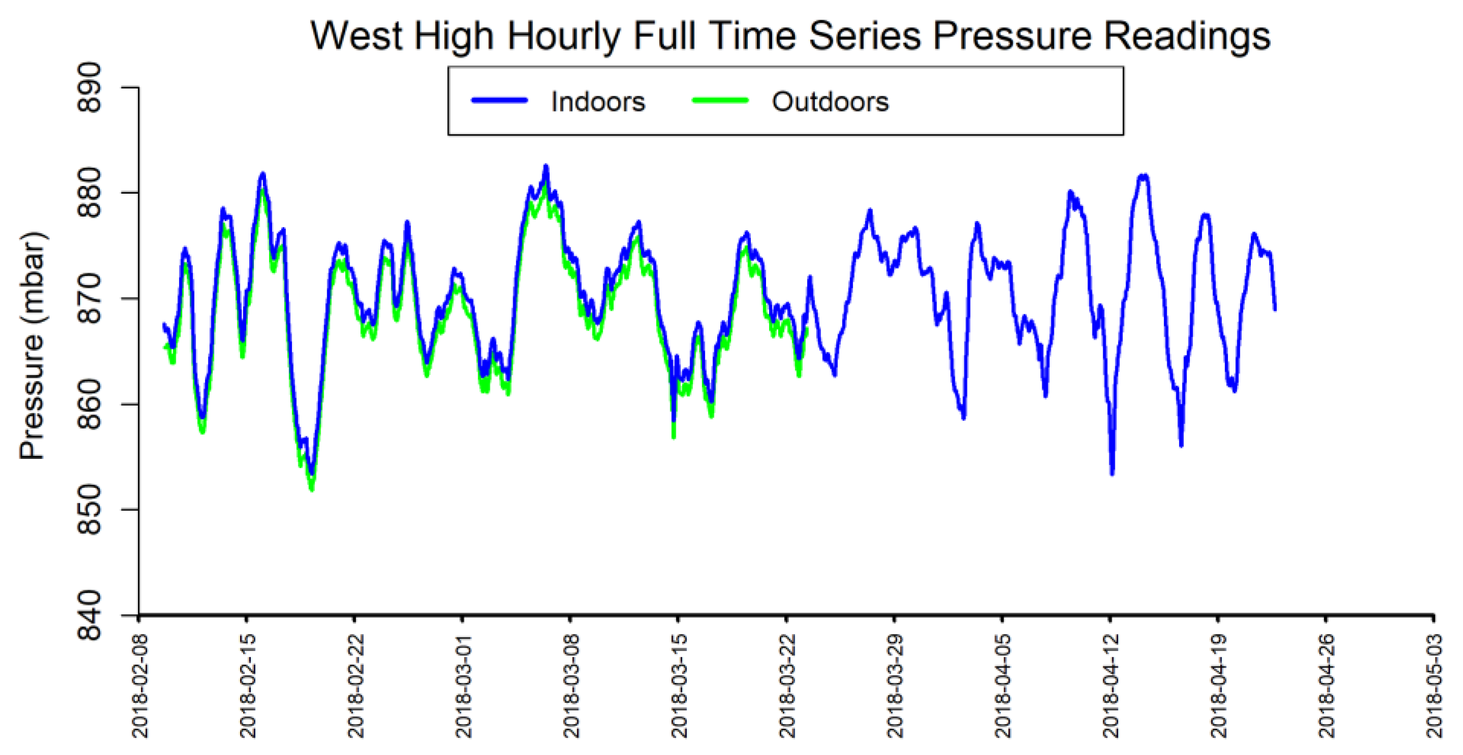
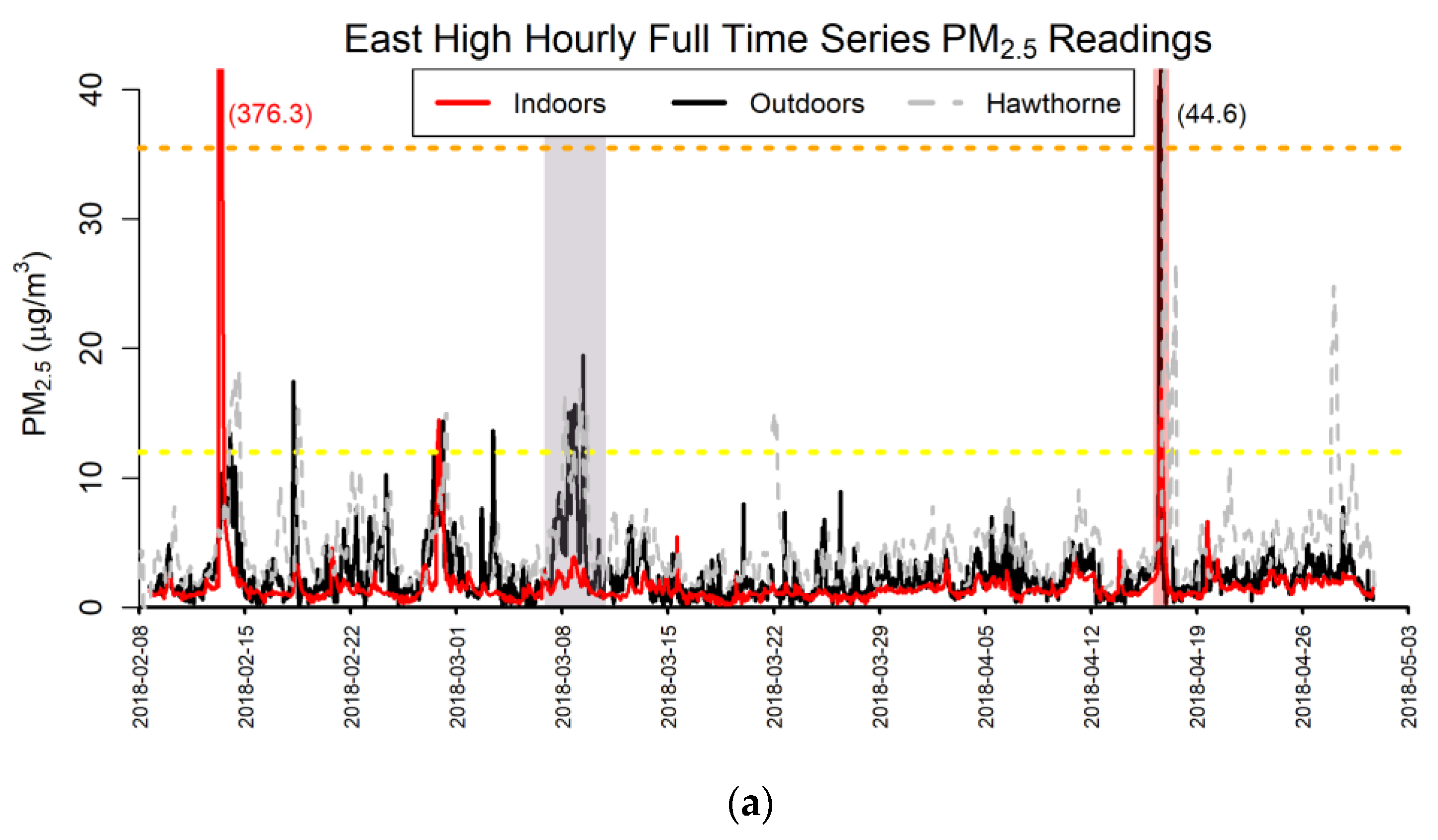
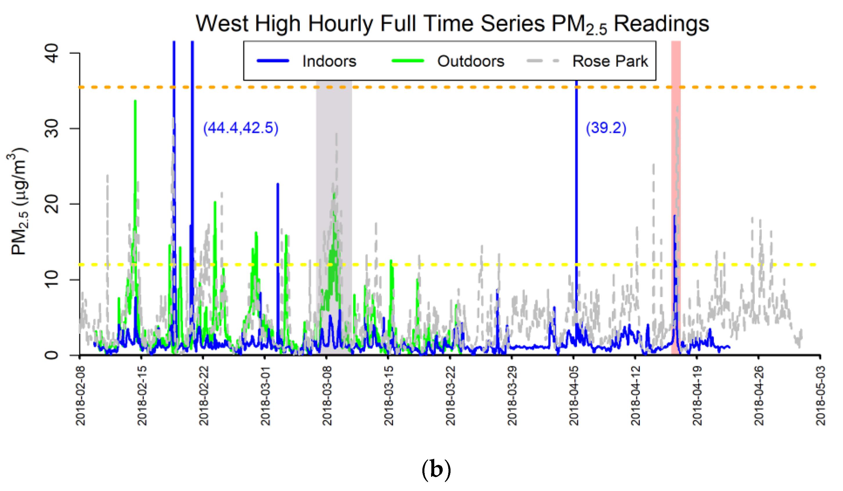
3.1. Full Time Series
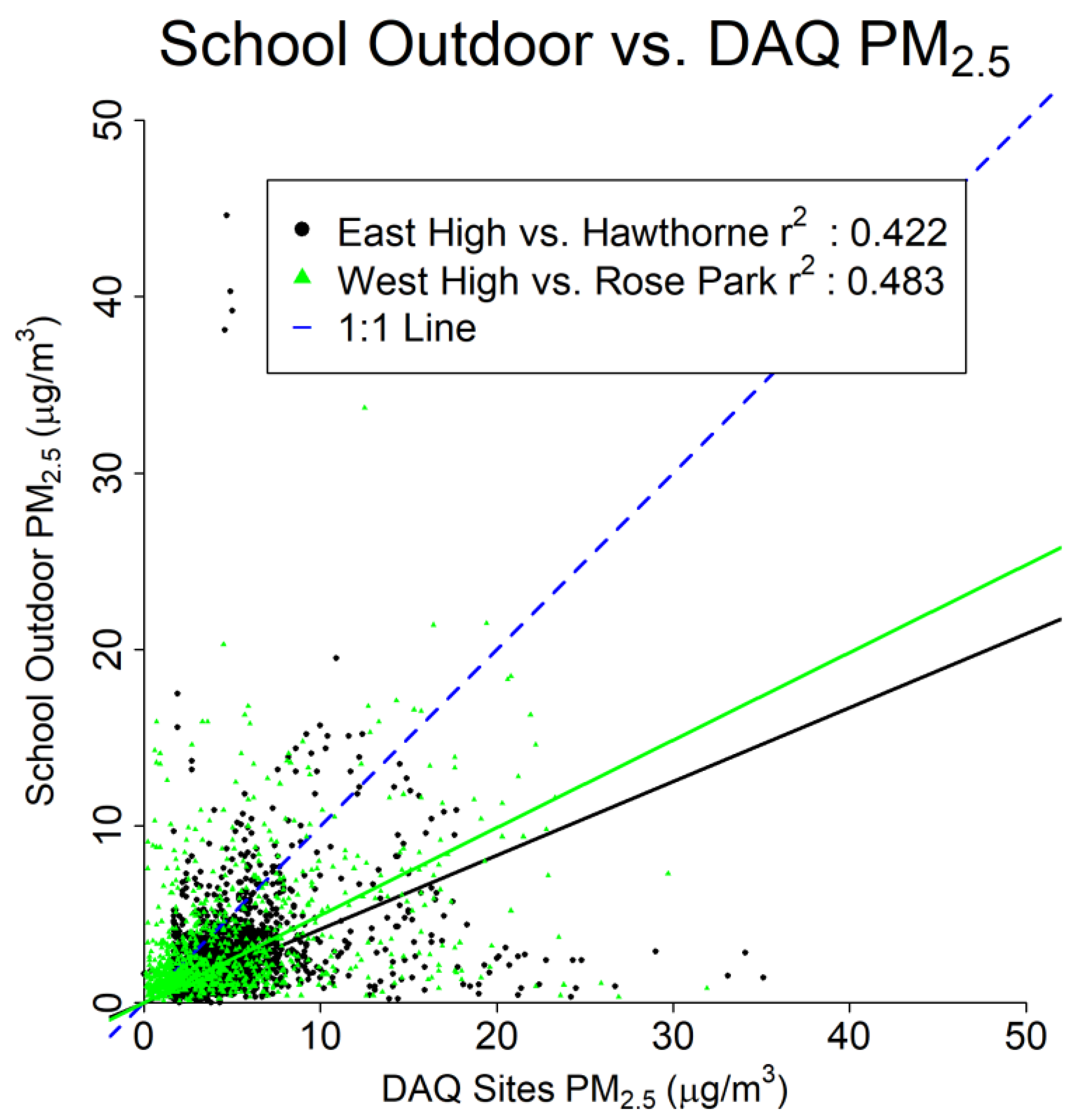
3.2. School Outdoor vs. Regulatory Sensor PM2.5
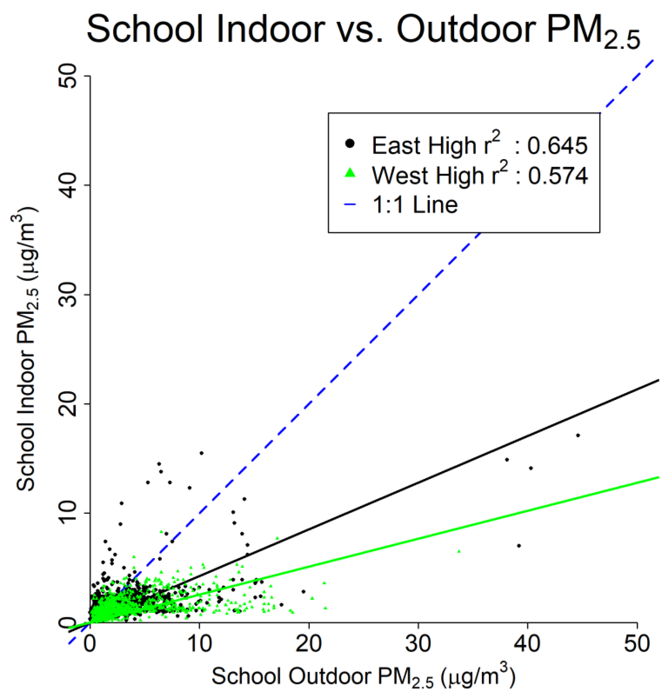
3.3. School Indoor vs. Outdoor PM2.5 Overview
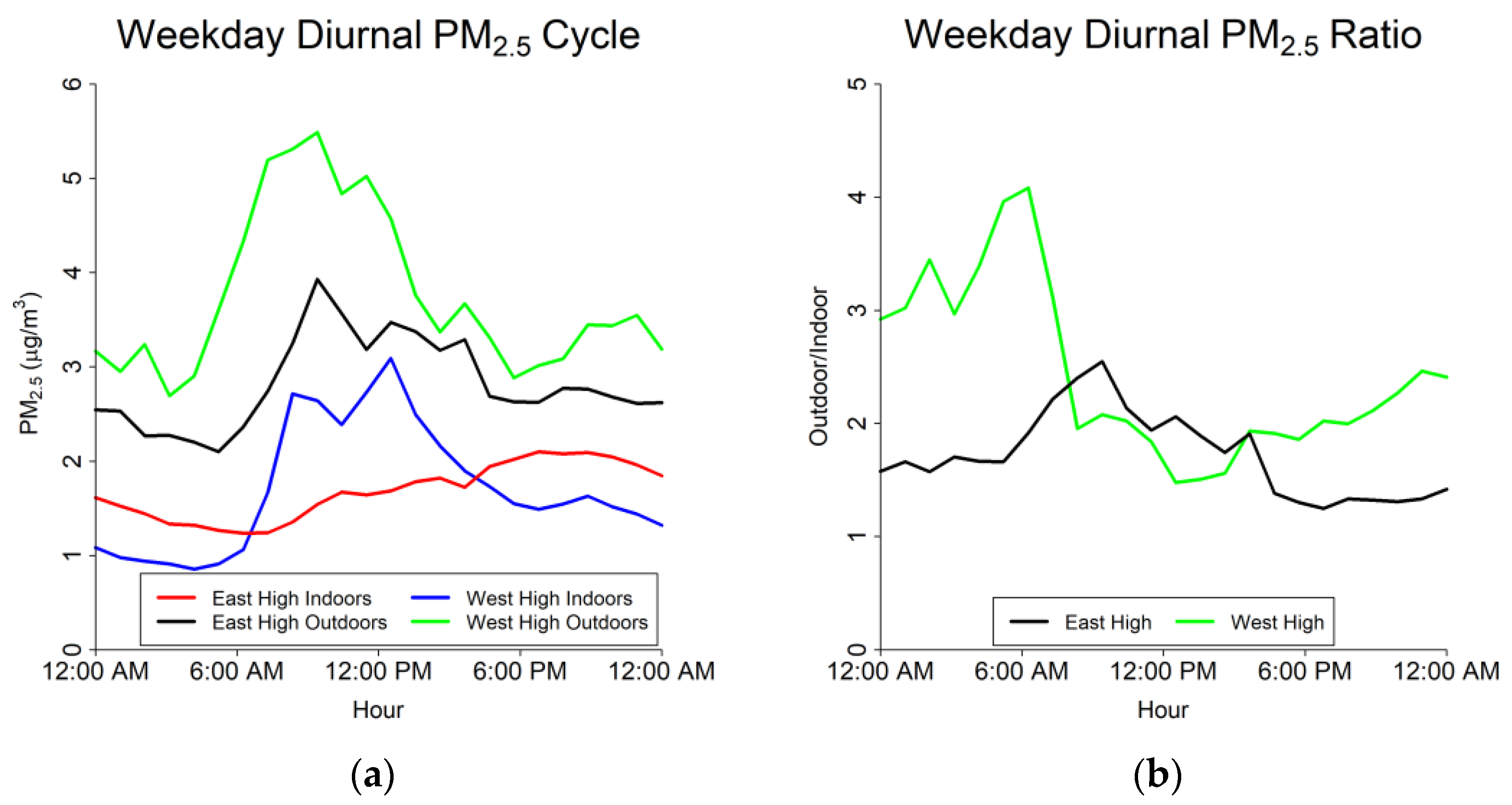
3.4. School Indoor vs. Outdoor PM2.5 and Weekday Diurnal Cycle
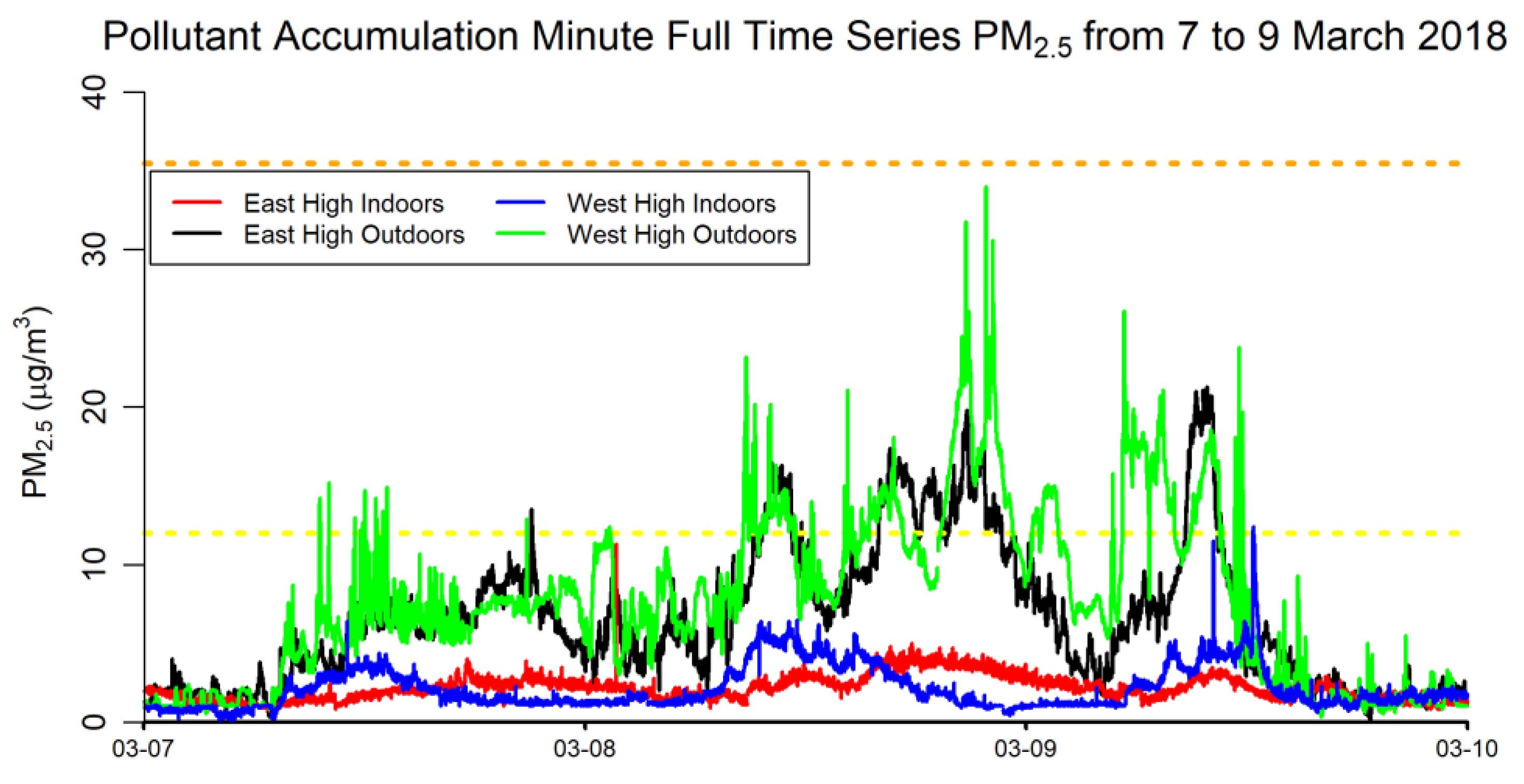
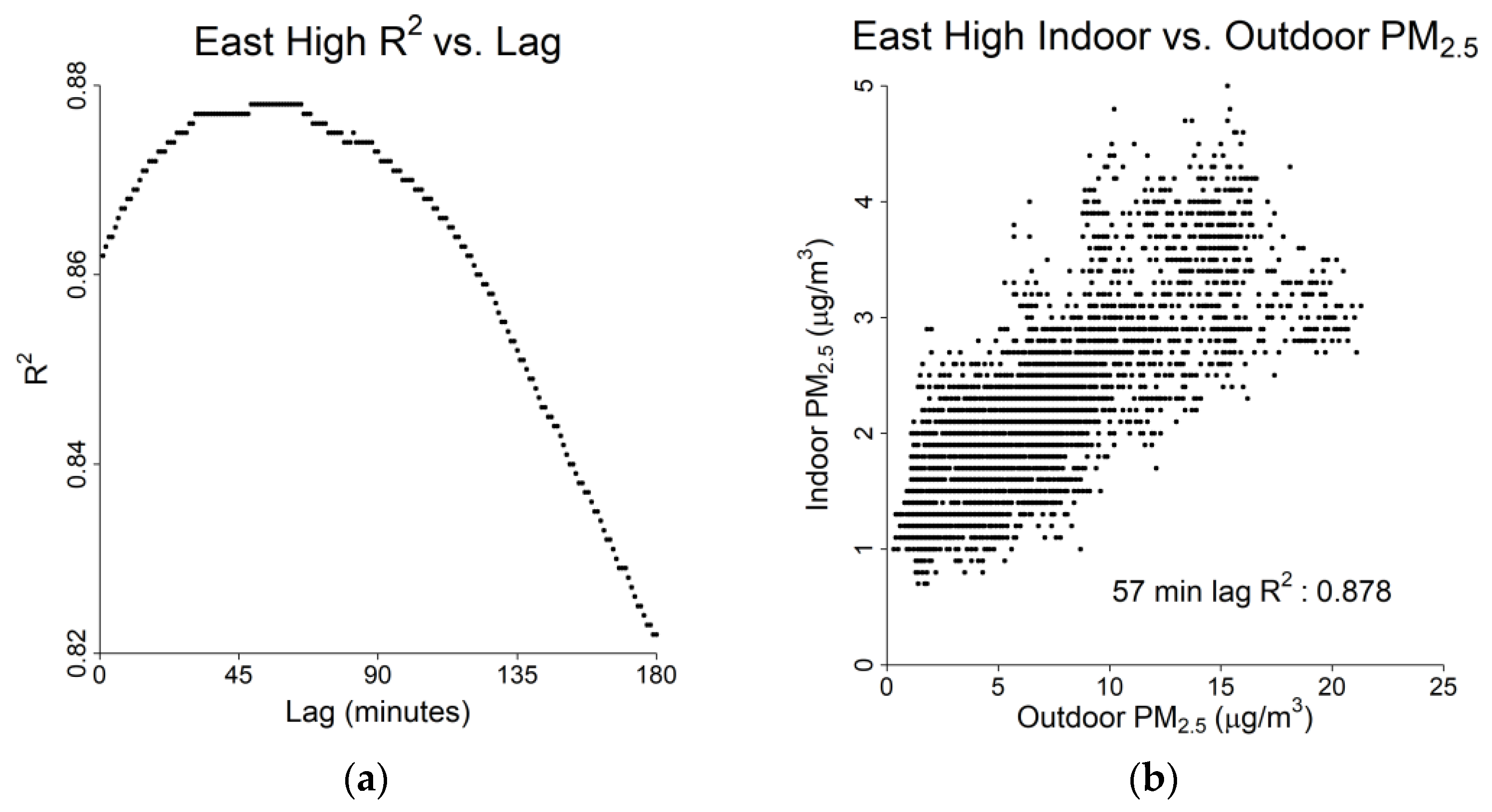
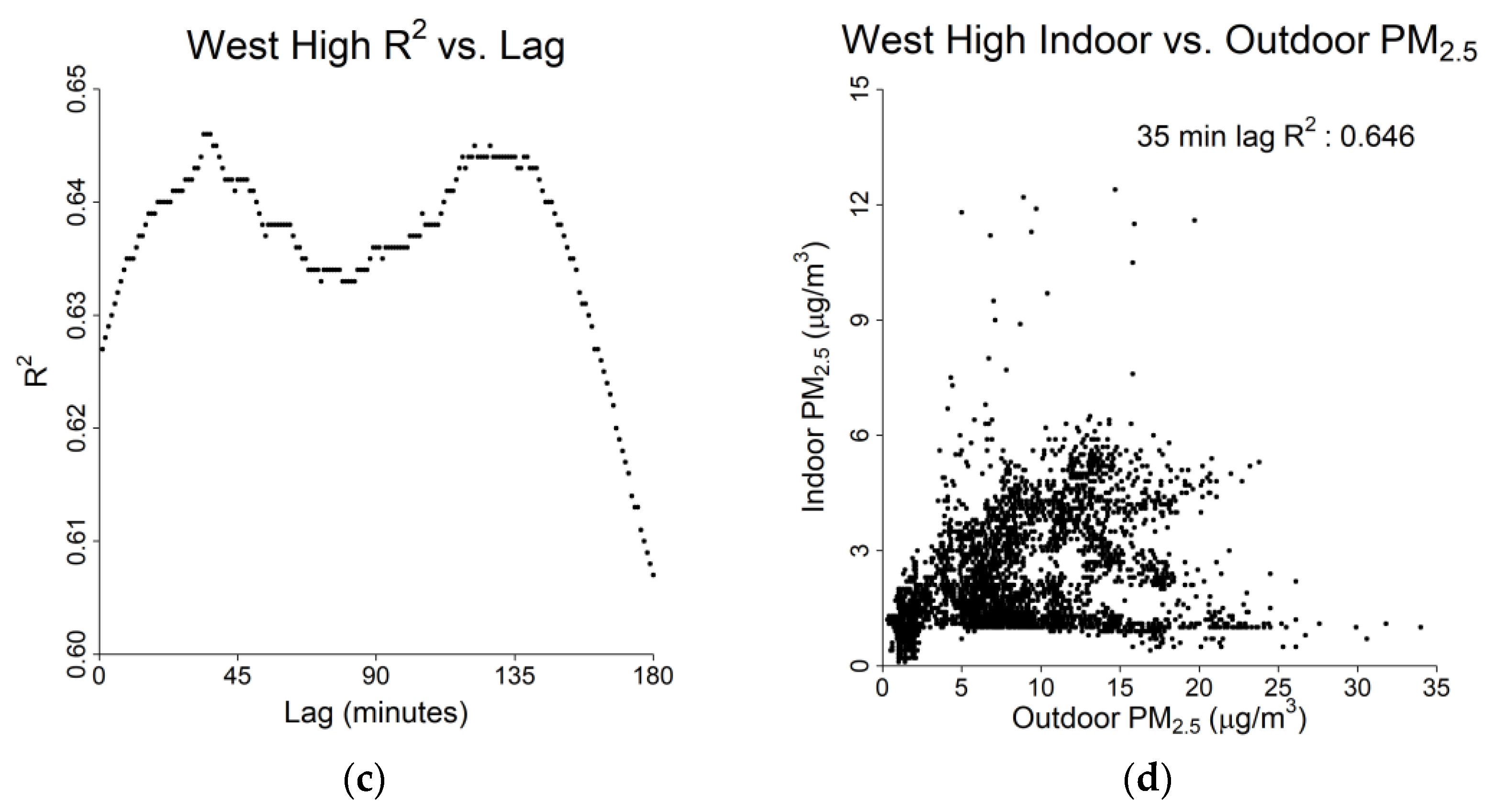
3.5. Pollutant Accumulation from 7 to 9 March—Atmospheric Inversion Event
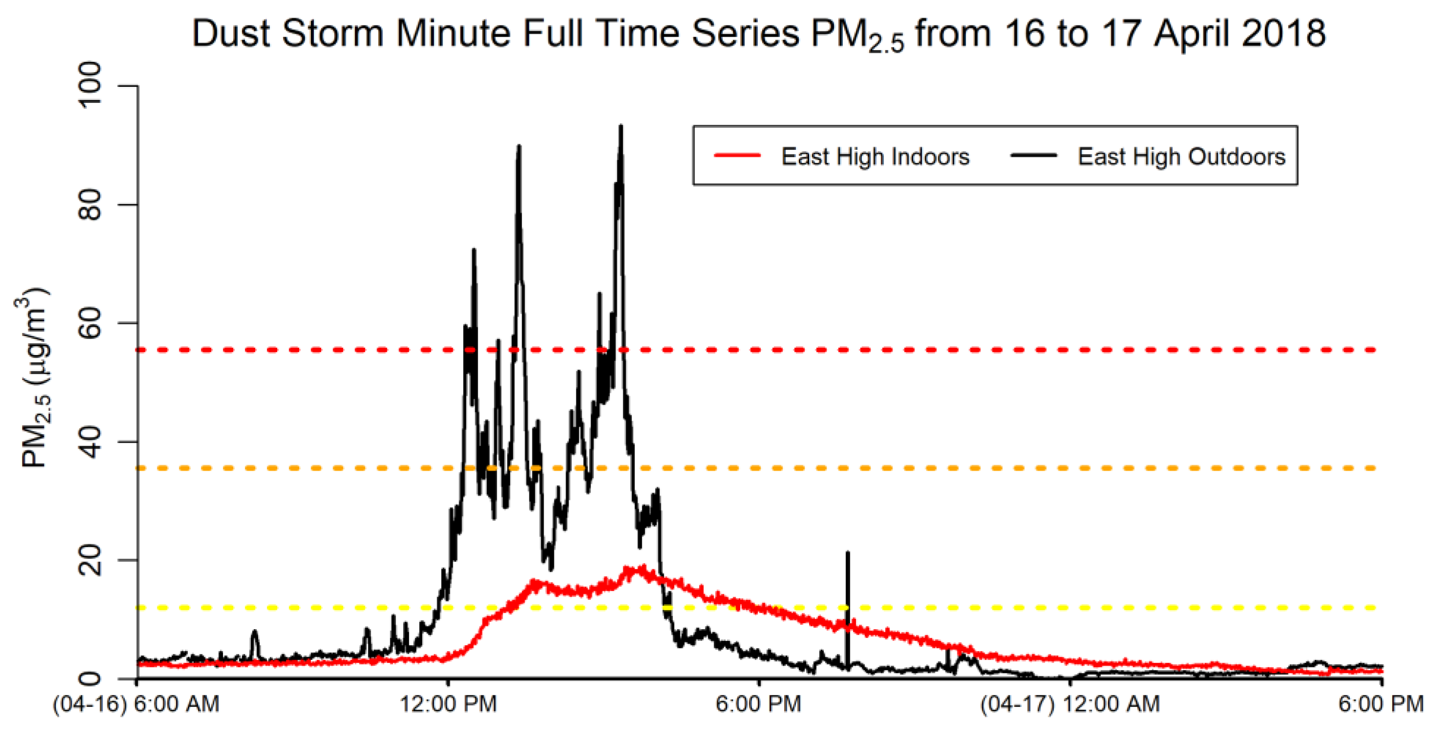
3.6. Dust Event on 16 April
4. Conclusions
4.1. Implications
4.2. Future Work
Author Contributions
Funding
Institutional Review Board Statement
Informed Consent Statement
Data Availability Statement
Acknowledgments
Conflicts of Interest
Appendix A

References
- WHO. Air Pollution And Child Health: Prescribing Clean Air; World Health Organization: Geneva, Switzerland, 2018. [Google Scholar]
- Gassebner, M.; Lamla, M.J.; Sturm, J.-E. Determinants of pollution: What do we really know? Oxf. Econ. Pap. 2011, 63, 568–595. [Google Scholar] [CrossRef] [PubMed]
- Hajat, A.; Hsia, C.; O’Neill, M.S. Socioeconomic Disparities and Air Pollution Exposure: A Global Review. Curr. Environ. Health Rep. 2015, 2, 440–450. [Google Scholar] [CrossRef] [PubMed] [Green Version]
- Clark, L.P.; Millet, D.B.; Marshall, J.D. National patterns in environmental injustice and inequality: Outdoor NO2 air pollution in the United States. PLoS ONE 2014, 9, e94431. [Google Scholar] [CrossRef]
- Miller, S.; Vela, M. The Effects of Air Pollution on Educational Outcomes: Evidence from Chile; Inter-American Development Bank (IDB): Washington, DC, USA, 2013. [Google Scholar]
- Mullen, C.; Grineski, S.E.; Collins, T.W.; Mendoza, D.L. Effects of PM2.5 on Third Grade Students’ Proficiency in Math and English Language Arts. Int. J. Environ. Res. Public Health 2020, 17, 6931. [Google Scholar] [CrossRef]
- Mendoza, D.L.; Pirozzi, C.S.; Crosman, E.T.; Liou, T.G.; Zhang, Y.; Cleeves, J.J.; Bannister, S.C.; Anderegg, W.R.L.; Robert, P.I. Impact of low-level fine particulate matter and ozone exposure on absences in K-12 students and economic consequences. Environ. Res. Lett. 2020, 15, 114052. [Google Scholar] [CrossRef]
- Errigo, I.M.; Abbott, B.W.; Mendoza, D.L.; Mitchell, L.; Sayedi, S.S.; Glenn, J.; Kelly, K.E.; Beard, J.D.; Bratsman, S.; Carter, T.; et al. Human Health and Economic Costs of Air Pollution in Utah: An Expert Assessment. Atmosphere 2020, 11, 1238. [Google Scholar] [CrossRef]
- Landrigan, P.J.; Rauh, V.A.; Galvez, M.P. Environmental justice and the health of children. Mt. Sinai J. Med. J. Transl. Pers. Med. 2010, 77, 178–187. [Google Scholar] [CrossRef]
- Currie, J. Inequality at birth: Some causes and consequences. Am. Econ. Rev. 2011, 101, 1–22. [Google Scholar] [CrossRef] [Green Version]
- Sanders, N.J. What doesn’t kill you makes you weaker: Prenatal pollution exposure and educational outcomes. J. Hum. Resour. 2012, 47, 826–850. [Google Scholar] [CrossRef]
- Currie, J.; Zivin, J.G.; Mullins, J.; Neidell, M. What do we know about short-and long-term effects of early-life exposure to pollution? Annu. Rev. Resour. Econ. 2014, 6, 217–247. [Google Scholar] [CrossRef] [Green Version]
- Graff Zivin, J.; Neidell, M. Environment, health, and human capital. J. Econ. Lit. 2013, 51, 689–730. [Google Scholar] [CrossRef]
- Isen, A.; Rossin-Slater, M.; Walker, W.R. Every breath you take—Every dollar you’ll make: The long-term consequences of the clean air act of 1970. J. Political Econ. 2017, 125, 848–902. [Google Scholar] [CrossRef] [Green Version]
- Brauer, M. How much, how long, what, and where: Air pollution exposure assessment for epidemiologic studies of respiratory disease. Proc. Am. Thorac. Soc. 2010, 7, 111–115. [Google Scholar] [CrossRef] [PubMed]
- DeVries, R.; Kriebel, D.; Sama, S. Outdoor air pollution and COPD-related emergency department visits, hospital admissions, and mortality: A meta-analysis. COPD J. Chronic Obstr. Pulm. Dis. 2017, 14, 113–121. [Google Scholar] [CrossRef]
- McCreanor, J.; Cullinan, P.; Nieuwenhuijsen, M.J.; Stewart-Evans, J.; Malliarou, E.; Jarup, L.; Harrington, R.; Svartengren, M.; Han, I.-K.; Ohman-Strickland, P.; et al. Respiratory effects of exposure to diesel traffic in persons with asthma. N. Engl. J. Med. 2007, 357, 2348–2358. [Google Scholar] [CrossRef] [Green Version]
- Zanobetti, A.; Schwartz, J. The effect of fine and coarse particulate air pollution on mortality: A national analysis. Environ. Health Perspect. 2009, 117, 898–903. [Google Scholar] [CrossRef] [Green Version]
- Liu, L.; Poon, R.; Chen, L.; Frescura, A.-M.; Montuschi, P.; Ciabattoni, G.; Wheeler, A.; Dales, R. Acute effects of air pollution on pulmonary function, airway inflammation, and oxidative stress in asthmatic children. Environ. Health Perspect. 2009, 117, 668–674. [Google Scholar] [CrossRef]
- Santana, J.C.C.; Miranda, A.C.; Souza, L.; Yamamura, C.L.K.; Coelho, D.d.F.; Tambourgi, E.B.; Berssaneti, F.T.; Ho, L.L. Clean production of biofuel from waste cooking oil to reduce emissions, fuel cost, and respiratory disease hospitalizations. Sustainability 2021, 13, 9185. [Google Scholar] [CrossRef]
- García, E.; Weiss, E. Student Absenteeism: Who Misses School and How Missing School Matters for Performance; Economic Policy Institute: Washington, DC, USA, 2018. [Google Scholar]
- Mendoza, D.L.; Benney, T.M.; Boll, S. Long-term analysis of the relationships between indoor and outdoor fine particulate pollution: A case study using research grade sensors. Sci. Total Environ. 2021, 776, 145778. [Google Scholar] [CrossRef]
- Vardoulakis, S.; Giagloglou, E.; Steinle, S.; Davis, A.; Sleeuwenhoek, A.; Galea, K.S.; Dixon, K.; Crawford, J.O. Indoor exposure to selected air pollutants in the home environment: A systematic review. Int. J. Environ. Res. Public Health 2020, 17, 8972. [Google Scholar] [CrossRef]
- American Lung Association. State of the Air 2021; American Lung Association: Chicago, IL, USA, 2021. [Google Scholar]
- Pishue, B. INRIX 2020 Global Traffic Score Card; INRIX Research: Kirkland, WA, USA, 2020. [Google Scholar]
- Horel, J.; Crosman, E.T.; Jacques, A.; Blaylock, B.; Arens, S.; Long, A.; Sohl, J.; Martin, R. Summer ozone concentrations in the vicinity of the Great Salt Lake. Atmos. Sci. Lett. 2016, 17, 480–486. [Google Scholar] [CrossRef]
- Whiteman, C.D.; Hoch, S.W.; Horel, J.D.; Charland, A. Relationship between particulate air pollution and meteorological variables in Utah’s Salt Lake Valley. Atmos. Environ. 2014, 94, 742–753. [Google Scholar] [CrossRef]
- Mendoza, D.L.; Crosman, E.T.; Mitchell, L.E.; Jacques, A.; Fasoli, B.; Park, A.M.; Lin, J.C.; Horel, J. The TRAX Light-Rail Train Air Quality Observation Project. Urban Sci. 2019, 3, 108. [Google Scholar] [CrossRef] [Green Version]
- Bulot, F.M.J.; Russell, H.S.; Rezaei, M.; Johnson, M.S.; Ossont, S.J.J.; Morris, A.K.R.; Basford, P.J.; Easton, N.H.C.; Foster, G.L.; Loxham, M.; et al. Laboratory comparison of low-cost particulate matter sensors to measure transient events of pollution. Sensors 2020, 20, 2219. [Google Scholar] [CrossRef] [Green Version]
- ES-642; Dust Monitor Operation Manual. Met One Instruments, Inc.: Grants Pass, OR, USA, 2013.
- Google Maps. Available online: https://www.google.com/maps (accessed on 26 December 2021).
- USGS TNM Elevation Tool. Available online: https://apps.nationalmap.gov/elevation/ (accessed on 26 December 2021).
- Lareau, N.P.; Crosman, E.; Whiteman, C.D.; Horel, J.D.; Hoch, S.W.; Brown, W.O.; Horst, T.W. The persistent cold-air pool study. Bull. Am. Meteorol. Soc. 2013, 94, 51–63. [Google Scholar] [CrossRef] [Green Version]
- Steenburgh, W.J.; Massey, J.D.; Painter, T.H. Episodic dust events of Utah’s Wasatch Front and adjoining region. J. Appl. Meteorol. Climatol. 2012, 51, 1654–1669. [Google Scholar] [CrossRef] [Green Version]
- United States Environmental Protection Agency. Air Quality Index (AQI) Basics. Available online: https://www.airnow.gov/aqi/aqi-basics/ (accessed on 2 January 2022).
- Siegel, J.A.; Nazaroff, W.W. Predicting particle deposition on HVAC heat exchangers. Atmos. Environ. 2003, 37, 5587–5596. [Google Scholar] [CrossRef] [Green Version]
- Deng, S.; Lau, J. Seasonal variations of indoor air quality and thermal conditions and their correlations in 220 classrooms in the Midwestern United States. Build. Environ. 2019, 157, 79–88. [Google Scholar] [CrossRef]
- Zhang, J.J.; Wei, Y.; Fang, Z. Ozone pollution: A major health hazard worldwide. Front. Immunol. 2019, 2518. [Google Scholar] [CrossRef] [Green Version]


| Study Site | Metric | Mean | Standard Deviation |
|---|---|---|---|
| East High Indoors | PM2.5 (μg/m3) | 1.84 | 0.83 |
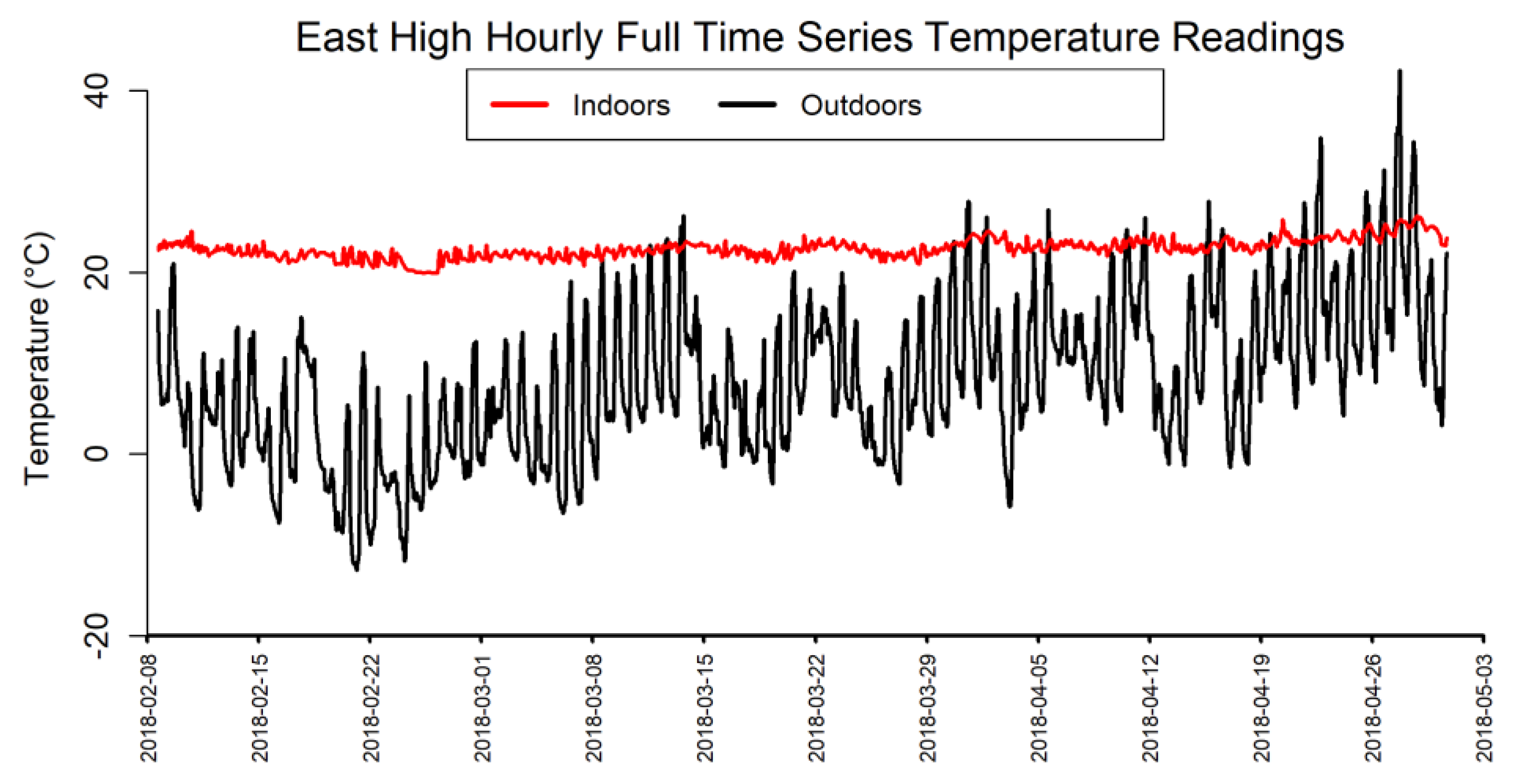
| Temperature (°C) | 22.01 | 0.49 | |
| Relative Humidity (%) | 15.60 | 1.53 | |
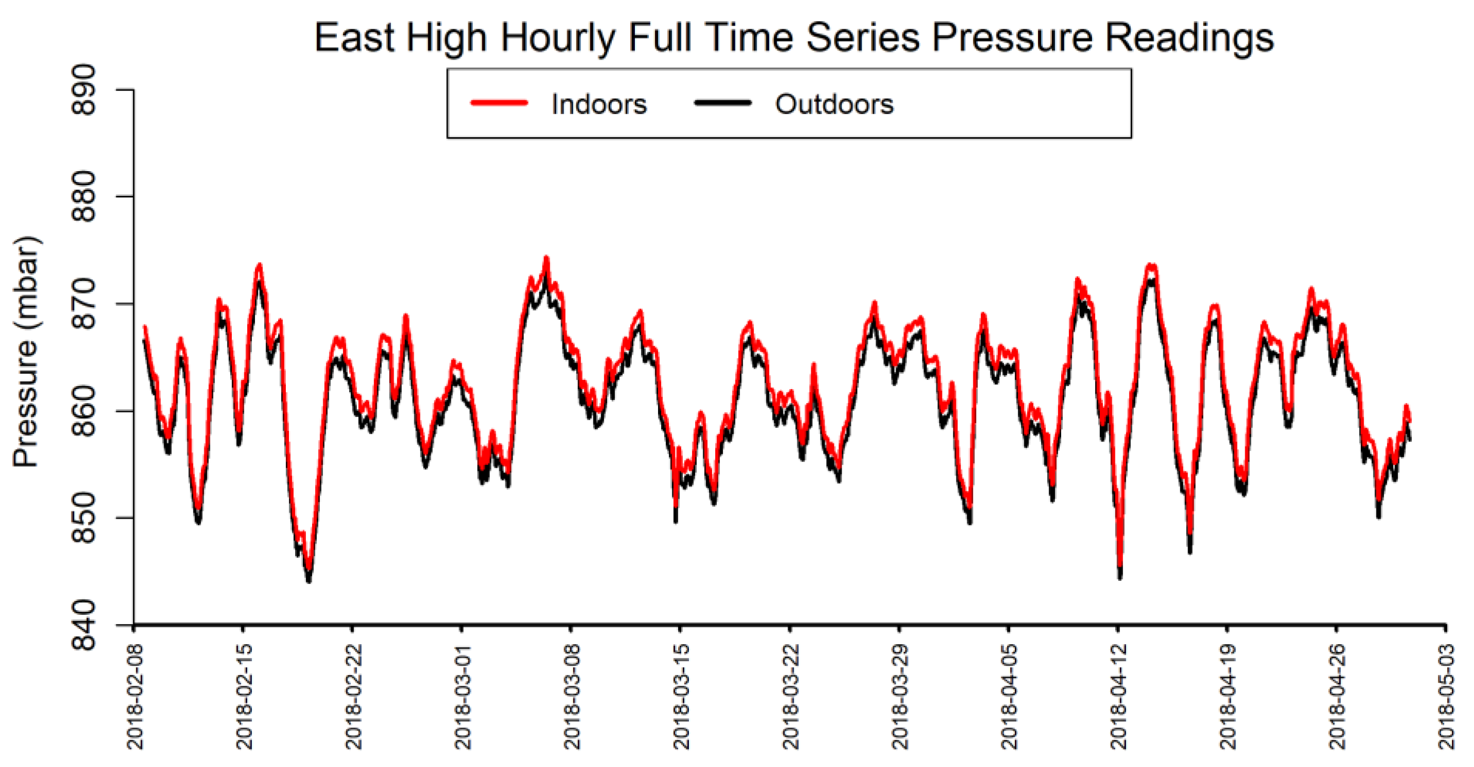
| Pressure (mbar) | 866.12 | 4.56 | |
| East High Outdoors | PM2.5 (μg/m3) | 4.89 | 4.30 |
| Temperature (°C) | 6.58 | 8.27 | |
| Relative Humidity (%) | 29.92 | 10.49 | |
| Pressure (mbar) | 864.65 | 4.45 | |
| West High Indoors | PM2.5 (μg/m3) | 1.79 | 1.26 |
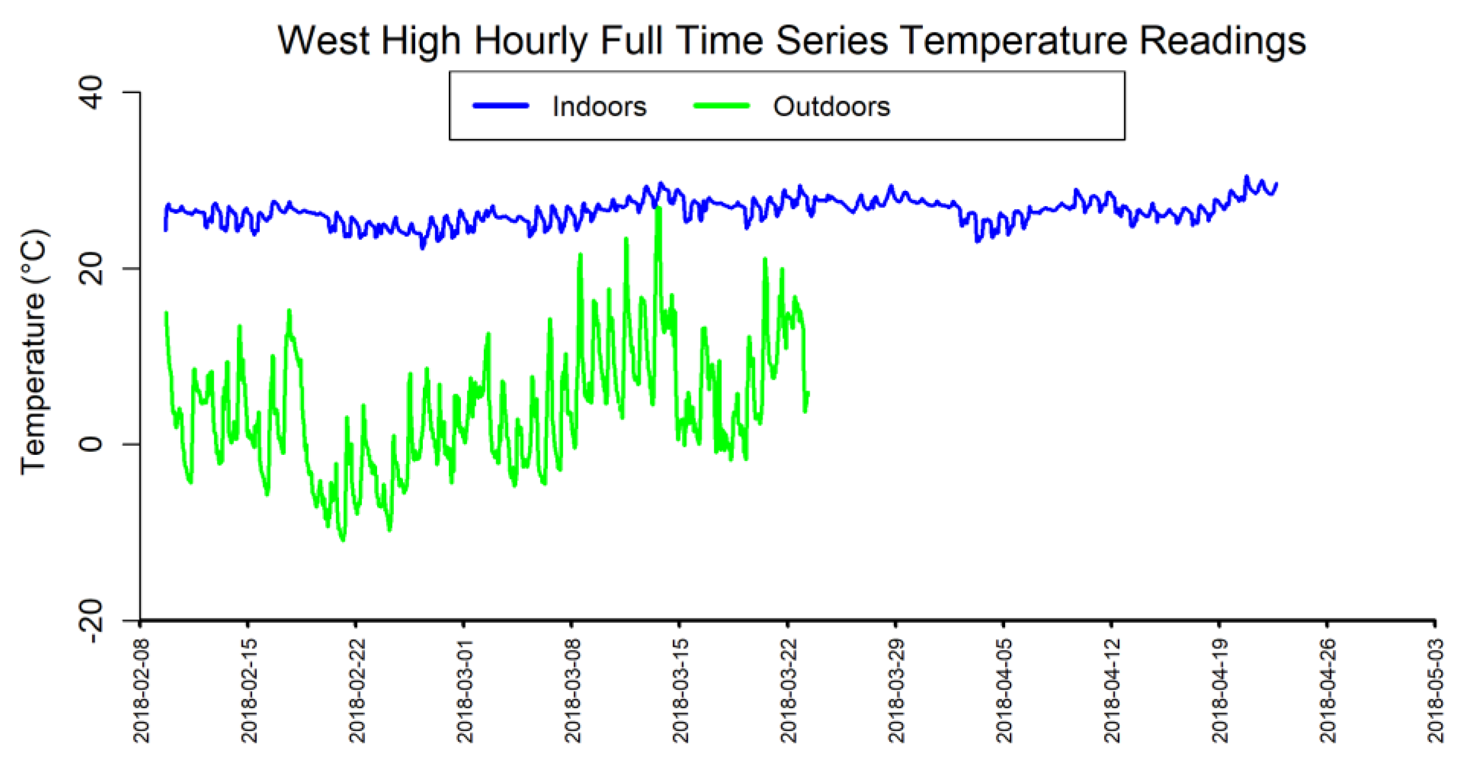
| Temperature (°C) | 26.02 | 0.93 | |
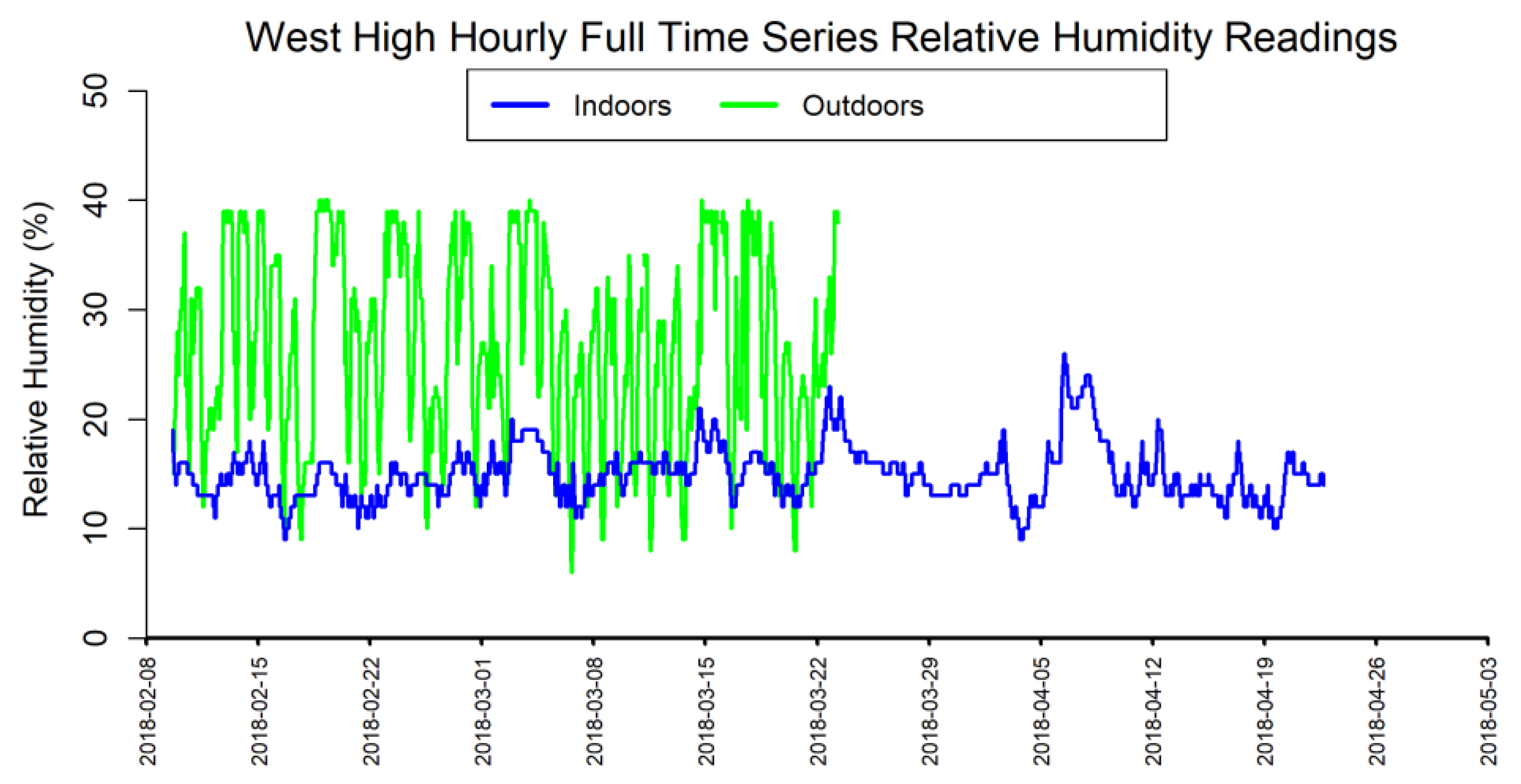
| Relative Humidity (%) | 14.15 | 1.49 | |
| Pressure (mbar) | 874.12 | 4.69 | |
| West High Outdoors | PM2.5 (μg/m3) | 5.61 | 5.19 |
| Temperature (°C) | 6.61 | 6.35 | |
| Relative Humidity (%) | 21.90 | 7.33 | |
| Pressure (mbar) | 872.66 | 4.70 |
Publisher’s Note: MDPI stays neutral with regard to jurisdictional claims in published maps and institutional affiliations. |
© 2022 by the authors. Licensee MDPI, Basel, Switzerland. This article is an open access article distributed under the terms and conditions of the Creative Commons Attribution (CC BY) license (https://creativecommons.org/licenses/by/4.0/).
Share and Cite
Mendoza, D.L.; Benney, T.M.; Bares, R.; Fasoli, B.; Anderson, C.; Gonzales, S.A.; Crosman, E.T.; Hoch, S. Investigation of Indoor and Outdoor Fine Particulate Matter Concentrations in Schools in Salt Lake City, Utah. Pollutants 2022, 2, 82-97. https://doi.org/10.3390/pollutants2010009
Mendoza DL, Benney TM, Bares R, Fasoli B, Anderson C, Gonzales SA, Crosman ET, Hoch S. Investigation of Indoor and Outdoor Fine Particulate Matter Concentrations in Schools in Salt Lake City, Utah. Pollutants. 2022; 2(1):82-97. https://doi.org/10.3390/pollutants2010009
Chicago/Turabian StyleMendoza, Daniel L., Tabitha M. Benney, Ryan Bares, Benjamin Fasoli, Corbin Anderson, Shawn A. Gonzales, Erik T. Crosman, and Sebastian Hoch. 2022. "Investigation of Indoor and Outdoor Fine Particulate Matter Concentrations in Schools in Salt Lake City, Utah" Pollutants 2, no. 1: 82-97. https://doi.org/10.3390/pollutants2010009
APA StyleMendoza, D. L., Benney, T. M., Bares, R., Fasoli, B., Anderson, C., Gonzales, S. A., Crosman, E. T., & Hoch, S. (2022). Investigation of Indoor and Outdoor Fine Particulate Matter Concentrations in Schools in Salt Lake City, Utah. Pollutants, 2(1), 82-97. https://doi.org/10.3390/pollutants2010009