Abstract
In this study, the application of adaptive fuzzy inference systems (ANFISs) and artificial neural networks (NNs) for grade and reserve estimation of a copper deposit was studied. More specifically, a feedforward NN with backpropagation and two Sugeno- type ANFIS were developed for grade and reserve estimation. Borehole assay data were used for training, validation, and testing of the NN and ANFIS. Grade estimates and tonnage–grade curves were produced and compared to those obtained using a geostatistical approach (Kriging).
Published: 22 March 2022
1. Introduction
Accurate mineral resource estimation is an essential step in evaluating the feasibility of any mining operation. The estimation of the quantity and quality of a mineral resource is traditionally performed using a model of selected deposit attributes, created by discretizing the deposit area into small blocks. The existing estimation methods include different techniques such as inverse distance weighing, kriging, and its various versions and stochastic simulations. These methods require an assumption in relation to the spatial correlation between samples to be estimated at non-sampled locations. In many cases, due to the complex relationships between the quality distribution and spatial pattern variability, the above-mentioned methods may not provide good estimation results.
Machine learning, and more specifically artificial neural networks (NNs) and adaptive neuro fuzzy inference systems (ANFISs), provide an approach for the estimation of mineral reserves. Since NNs and ANFISs are not only trainable nonlinear dynamic systems, but also adaptive model-free estimators, no assumption concerning the spatial variation of the deposit attributes need to be made. The basic approach for developing NN and ANFIS models for mineral reserves estimation is to train them using an existing borehole dataset of a mineral deposit and appropriate learning methods [1,2,3,4,5].
In this study, the application of NN and ANFIS and the issues involved with using them for reserve estimation were elaborated with the help of a drill-hole dataset of a copper deposit. The estimation of the grade and reserves of a copper deposit was conducted by using a feedforward with backpropagation NN and Sugeno type ANFIS. Borehole assay data were regularized into composites of equal length and then used for grade and reserves estimation. These data formed the set used for the training, validation, and testing of NNs and ANFISs, while the early stopping technique (described in Section 3.3) was used to avoid overtraining.
The resulting cooper concentration maps and tonnage–grade curves were estimated and compared to those obtained by using the geostatistical approach (kriging).
2. Artificial Neural Networks (NNs) and Adaptive Neuro-Fuzzy Inference Systems (ANFISs)
2.1. Artificial Neural Networks (NNs)
An artificial neural network is a computational structure inspired by the study of biological neural processing. It exhibits certain brain-like capabilities including perception, pattern recognition, and prediction in a variety of situations. As in the brain, information processing is conducted in parallel using a network of ‘neurons’. Therefore, neural networks have capabilities that go beyond algorithmic programming and work very well for nonlinear input–output mapping. It is this property of nonlinear mapping by the neural network, which can be explored for ore grade estimation.
Basically, three entities characterize a neural network: the characteristics of the individual neuron, the network topology, and the learning strategy. Each processing unit (neuron) receives one or more inputs and delivers a single output. The neuron consists of an input function (a summation function), the result of which is fed to the activation function, which in turn determines the output. The topology of the network is the manner in which neurons are organized and connected. Neurons are combined to form layers that can be connected fully or partially. When the output from every neuron of a particular layer is connected to every neuron in the next layer, the network is fully connected, otherwise, it is partially connected. Associated with each connection between these processing units, there is a weight value defined to represent the connection strength. Each network has an input layer, which accepts the input data to the network, an input layer that delivers the network response, and the intermediate layers that represent the hidden features of the problem [6].
Feedforward networks are those in which the output from a neuron can only feed forward, while feedback networks are those in which the output from a neuron can be directed back as an input to any neuron. Learning methods for neural networks can be classified into supervised and unsupervised. The most commonly used supervised method for feedforward neural networks is backpropagation.
The final output is compared to the desired value from the training set. The error is computed as the difference between the desired and actual output. This error is propagated backward through the network and weight changes are made throughout, according to an algorithm to minimize error.
The process of modifying weights in response to sets of input and desired outputs is called learning. Training a network involves this iterative process until the error either converges to a predetermined threshold or stabilizes [6]. At this point, input data never seen by the ANN can be presented to observe the output generated.
2.2. Adaptive Neuro-Fuzzy Inference Systems (ANFISs)
Adaptive neuro-fuzzy inference system, which was proposed by Jang (1993) [7], Jang and Sun (1995) [8], Jang et al. (1998) [9], is a combination of a fuzzy inference system (FIS) and neural network and has the advantages of both techniques. This combination employs a fuzzy system to represent knowledge in an interpretable way and a neural network to adjust the membership function parameters and linguistic rules directly from data in such a way that the system’s performance will be enhanced [10].
While in common fuzzy inference systems the membership functions and rule structure are chosen initially somewhat arbitrarily and then are tuned by utilizing the experts’ knowledge, in adaptive neuro-fuzzy inference systems, a given input/output dataset is used to construct a fuzzy inference system. ANFIS membership function parameters are selected and adjusted using either a backpropagation algorithm alone, or in combination with a least squares type of method [11]. This allows ANFIS to learn from the data and have a structure similar to that of a neural network. ANFIS maps inputs through membership functions and associated parameters to outputs. The parameters associated with the membership functions change through the learning process. The adjustment of these parameters is facilitated by a gradient vector, which provides a measure of how well the fuzzy inference system is modeling the input/output data for a given set of parameters. Since ANFIS is more complex than common fuzzy inference systems, a zero- or first order Sugeno-type system with a single output is preferred rather than higher order. Higher order Sugeno type fuzzy models introduce significant complexity with little obvious merit. Sugeno type inference systems of zero- and first-order have the following general form [11]:
where x and y are the fuzzy input variables; A and B are the fuzzy sets in the antecedent; z is the output; and k, a, b, c are all constants. Output is obtained using the weighted average defuzzification method [11].
IF x is A and y is B THEN z = k (zero order)
IF x is A and y is B THEN z = ax + by + c (first order)
3. Model Development, Training and Testing
3.1. NN Development
In this study, the estimation of the grade and reserves of a copper deposit was conducted by using a fully interconnected feedforward NN. As shown in Figure 1, the developed NN had an input layer with three neurons, a hidden layer of m neurons, and an output layer with one neuron. The coordinates of each drill hole composite sample were used as inputs, while the logged value of content (%) in Cu was used as the output. The optimal number m of hidden layer neurons was evaluated during training while the bias (ao, bo,j) was used to improve the accuracy of the estimation.
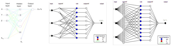
Figure 1.
Structure of NN and ANFIS used for ore reserve estimation. (left) Multiple-layer feedforward neural network, (center) ANFIS generated by grid partition, and (right) ANFIS generated by sub clustering.
3.2. ANFIS Development
The strategy for the development of an ANFIS model was similar to that of the NN. The system was first designed using a first-order Sugeno fuzzy inference system. A first-order Sugeno fuzzy model can capture the variability in the data better than a zero-order Sugeno fuzzy model. It is a three input–one output system where the input variables are X, Y, and Z coordinates, while the log-transformed % Cu content is taken as the output variable. The final output of both NN and ANFIS was obtained by back-transforming the estimated log-transformed % Cu values.
Two different ANFIS models were developed using MATLAB software: the first was generated using the grid partition method and the second using the sub-clustering method (Figure 1). The method generates a Sugeno-type FIS structure used as the initial conditions (initialization of the membership function parameters) [12]. The subtractive clustering algorithm is another approach to generate ANFIS, which estimates the cluster number and the cluster location automatically [13]. The adjustment of membership function parameters (training) was performed by a hybrid method based on least squares and backpropagation algorithm.
3.3. Training, Validation, and Testing
One of the most common problems that may arise during training of a neural network is overtraining. Overtraining occurs when models are very well trained in the details and noise of all data, but cannot generalize the acquired knowledge and thus their performance is low when checking their reliability with new data not used in education. To solve this problem, a commonly used technique, known as early stopping, is to stop the training on time by using an additional dataset (validation set) that is used to control the training without having its data participating in it. During the training process, the estimation error gradually decreases with the passing of the epochs for the whole training data. In contrast the validation dataset error decreases to a minimum value and then increases. At this point, the minimum error for the validation dataset, the neural network training stops to avoid overtraining. Finally, a third dataset, named testing, is presented to the trained model to test the accuracy of the prediction for unknown data not involved in training [11].
3.4. Dataset
The examined Andina copper deposit is located 80 km northeast of Santiago in Chile’s Region V and is described in detail by Hustrulid and Kuchta (2006) [14]. The Andina Division operates two mines: Rio Blanco, a panel caving operation, and Sur Sur, an open pit. The Sur Sur orebody represents a hydrothermal breccia complex. Several breccia types can be defined based upon clast size and composition, matrix and/or cement type, clast to matrix ratio, mineralization, and alteration. The orebody was explored through 76 boreholes of varying depth and their locations are shown in Figure 2a. Borehole assay data were regularized into composites of equal length and then used for grade and reserves estimation. The main statistical parameters and the histogram of Cu% values of the composite samples are shown in Figure 2b. Since the observed distribution of Cu% values was highly skewed, the logarithmic transformation was used. This transformation helped us to obtain a distribution very close to normal (Figure 2d) and to avoid the estimation of negative values of Cu % content (with NN and ANFIS) that have no natural meaning in this case. The experimental omnidirectional variogram of the log-transformed % Cu values of the composites samples, shown in Figure 2c, was modeled by an exponential model with parameters Co = 0.3 (nugget effect), C = 0.9 (sill), and range of influence a = 150 ft.
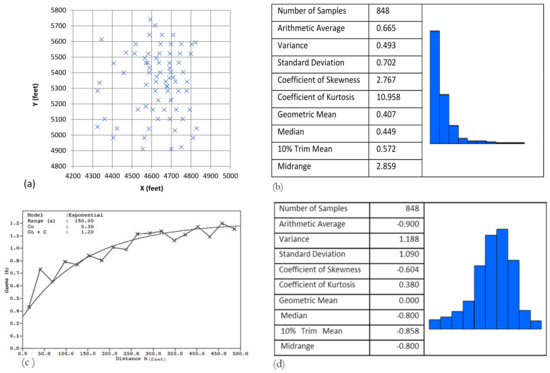
Figure 2.
(a) Location of drill holes for the exploration of the Andina cooper deposit. (b) Statistical parameters and distribution of Cu% values of the composite samples. (c) Omnidirectional experimental variogram of the log-transformed values of % Cu with the fitted exponential model. (d) Statistical parameters and distribution of the log-transformed values of Cu %.
For the development of NN and ANFIS, MATLAB software was implemented. The set of data used for training, validation, and testing consisted of 640 composite samples of Cu. Of these, 70% of the samples were used for the training, 15% for validation, and 15% for testing. Their separation was conducted in a random way.
4. Results and Discussion
The training results are summarized in Table 1, where the correlation coefficient R2 and the RMS error between actual and predicted values of Cu% content are shown. R2 values were relatively high, indicating that the developed models effectively captured the spatial variability of Cu % content. NN and ANFIS generated by grid partition were performed similarly and were slightly better compared to the ANFIS generated by sub-clustering.

Table 1.
Correlation coefficients and RMS errors between the actual and predicted values of Cu % for the NN and ANFIS models.
Next, the orebody was divided into small blocks (50 × 50 × 25 ft3) and for each block, the Cu % content was estimated by the trained NN and ANFIS. For comparison, the same calculations were carried out by using the ordinary kriging method. In all cases, the logarithmic transformation was applied to Cu % values.
The comparison of the results obtained from the different methods was based on the estimation of the correlation coefficients R2 among the estimated values of Cu % as well as on the calculated grade–reserves curves. The correlation coefficients (R2) shown in Table 2 indicate that the NN and the ANFIS (generated by grid partition) performed similarly. Additionally, the ANFIS generated by grid partition and NN had the strongest correlation with kriging. Regarding the grade–reserves curves, as shown in Figure 3, NN and ANFIS seemed to overestimate the reserves with Cu % content less than 0.5% and to underestimate the reserves with Cu % content greater than 0.5%.
Table 2.
R squared of Cu % values of blocks estimated by different methods (kriging, ANFIS, and NN).
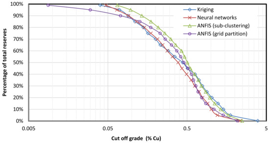
Figure 3.
Grade–reserves curves for the different applied estimation methods.
5. Conclusions
The results obtained from this study indicated that both NN and ANFIS have the potential to be used as ore reserve estimators. The observed overestimation of low grade blocks was associated with the large number of low grade borehole samples used during the training of the NN and ANFIS. Since NN and ANFIS are trainable data-driven systems, emphasis should be placed on the development of effective training methods capable of effectively capturing the spatial variability of the orebody grade.
Author Contributions
Conceptualization, M.G.; Methodology, M.G., A.V. and A.R.; Software, V.D.; Writing—original draft preparation, M.G. and A.V.; Writing—review and editing, S.R.; Supervision, M.G. All authors have read and agreed to the published version of the manuscript.
Funding
This research was funded by the “National Contribution to European competitive projects-BEWEXMIN” managed by the Research Committee of the Technical University of Crete, Grant number 82160.
Institutional Review Board Statement
Not applicable.
Informed Consent Statement
Not applicable.
Data Availability Statement
Not applicable
Conflicts of Interest
The authors declare no conflict of interest. The funders had no role in the design of the study; in the collection, analyses, or interpretation of data; in the writing of the manuscript, or in the decision to publish the results.
References
- Wu, X.; Zhou, Y. Reserve estimation using neural network techniques. Comput. Geosci. 1992, 19, 567–575. [Google Scholar] [CrossRef]
- Galetakis, M. Application of Artificial Neural Networks in Solving Problems Related with Open Pit Mine Planning and Design. Miner. Wealth 1999, 113, 47–56. [Google Scholar]
- Kapageridis, I. Input space configuration effects in neural network-based grade estimation. Comput. Geosci. 2005, 112, 704–717. [Google Scholar] [CrossRef]
- Samanta, B.; Bandopadhyay, S. Construction of a radial basis function network using an evolutionary algorithm for grade estimation in a placer gold deposit. Comput. Geosci. 2009, 35, 1592–1602. [Google Scholar] [CrossRef]
- Li, X.; Xie, Y.; Guo, Q.; Li, L. Adaptive ore grade estimation method for the mineral deposit evaluation. Math. Comput. Model. 2010, 52, 1947–1956. [Google Scholar] [CrossRef]
- Rumelhart, D.; Hinton, G.; Williams, R. Learning Internal Representations by Error Propagation, Parallel Distributed Processing; MIT Press: Cambridge, MA, USA, 1986; Volume 1, pp. 318–362. [Google Scholar]
- Jang, J.S. ANFIS: Adaptive-network-based fuzzy inference system. IEEE Trans. Syst. Man Cybern. 1993, 23, 665–685. [Google Scholar] [CrossRef]
- Jang, J.S.; Sun, C.T. Neuro-fuzzy modeling and control. Proc. IEEE 1995, 83, 378–406. [Google Scholar] [CrossRef]
- Jang, J.S.R.; Sun, C.T.; Mizutani, E.; Ho, Y. Neuro-fuzzy and soft computing-a computational approach to Learning and machine intelligence. Proc. IEEE 1998, 86, 600–603. [Google Scholar] [CrossRef]
- Wang, Z.; Palade, V.; Xu, Y. Neuro-fuzzy ensemble approach for microarray cancer gene expression data analysis. In Proceedings of the 2006 International Symposium on Evolving Fuzzy Systems, Ambelside, UK, 7–9 September 2006. [Google Scholar]
- Sugeno, M. Industrial Applications of Fuzzy Control; Elsevier Science Pub. Co.: Amsterdam, The Netherlands, 1985. [Google Scholar]
- Mathworks. Available online: https://www.mathworks.com/help/fuzzy/genfis1.html (accessed on 19 May 2021).
- Hiremath, S.M.; Patra, S.C.; Mishra, A.K. ANFIS with Subtractive Clustering-Based Extended Data Rate Prediction for Cognitive Radio. In Proceedings of the 5th International Conference on Computers and Devices for Communication, Rourkela, India, 17–19 December 2012. [Google Scholar]
- Hustrulid, W.; Kuchta, M. Open Pit Mine Planning & Design: CSMine Software Package, 2nd ed.; Taylor and Francis/Balkema: Abingdon, UK, 2006. [Google Scholar]
Publisher’s Note: MDPI stays neutral with regard to jurisdictional claims in published maps and institutional affiliations. |
© 2022 by the authors. Licensee MDPI, Basel, Switzerland. This article is an open access article distributed under the terms and conditions of the Creative Commons Attribution (CC BY) license (https://creativecommons.org/licenses/by/4.0/).