1. Introduction
The role of predictive maintenance, especially in dynamic parts of machines, is very crucial. In most modern-day industrial machines and robots, rolling elements like ball bearings play a pivotal role in the dynamic and smooth functioning of the machines. Faulty rotating parts emit signals with special patterns, and they can be thermal, acoustic, vibrational, pulsative, current, etc. The vibration signal can be obtained in various formats like displacement, velocity, and acceleration. For these formats, accelerometers are the most widely used sensors for signal acquisition [
1].
Effective vibrational analysis techniques like spectral kurtosis and envelope analysis are proven efficient and require separation of actual signals from noise [
2]. Empirical mode decomposition and wavelet transformations for fault diagnosis in rotating machinery were explored in [
3]. Variational mode decomposition and FCM clustering were analyzed to predict the bearing faults [
4]. A study investigated fault diagnosis using wavelet packet transformation (WPT)–FCM and other methods and revealed that WPT–FCM outperformed in terms of the accuracy of a vibration signal [
5]. A hybrid empirical wavelet transformation (EWT), AR, and FCM method for bearing fault diagnosis was used, and their accuracies were compared [
6].
Gear fault diagnosis was performed with an AR model for a wind turbine in [
7]. AR can extract information from both healthy as well as faulty signals and can reduce noise in the faulty signal [
8,
9]. A similar kind of study was conducted for gear shaft fault diagnosis [
10]. The authors of [
11] applied discrete wavelet packet analysis to extract the frequencies of interest. The data was then used to obtain AR coefficients. This method was able to achieve an improved signal-to-noise ratio. Industrial turbines have various sensors capturing data in real time. Fuzzy logic was implemented in [
12] to achieve fault detection in early stages. Lifting wavelet decomposition has been combined with Fuzzy C-means. Lifting wavelet packet decomposition is used to extract features [
13].
For comparison, an envelope analysis was carried out to obtain high-frequency components from the original signal for improved performance [
14]. This study potentially addresses these challenges and effectively provides promising outcomes for various fault predictions at different loads, speeds, and sensor orientations.
2. Experimental Setup
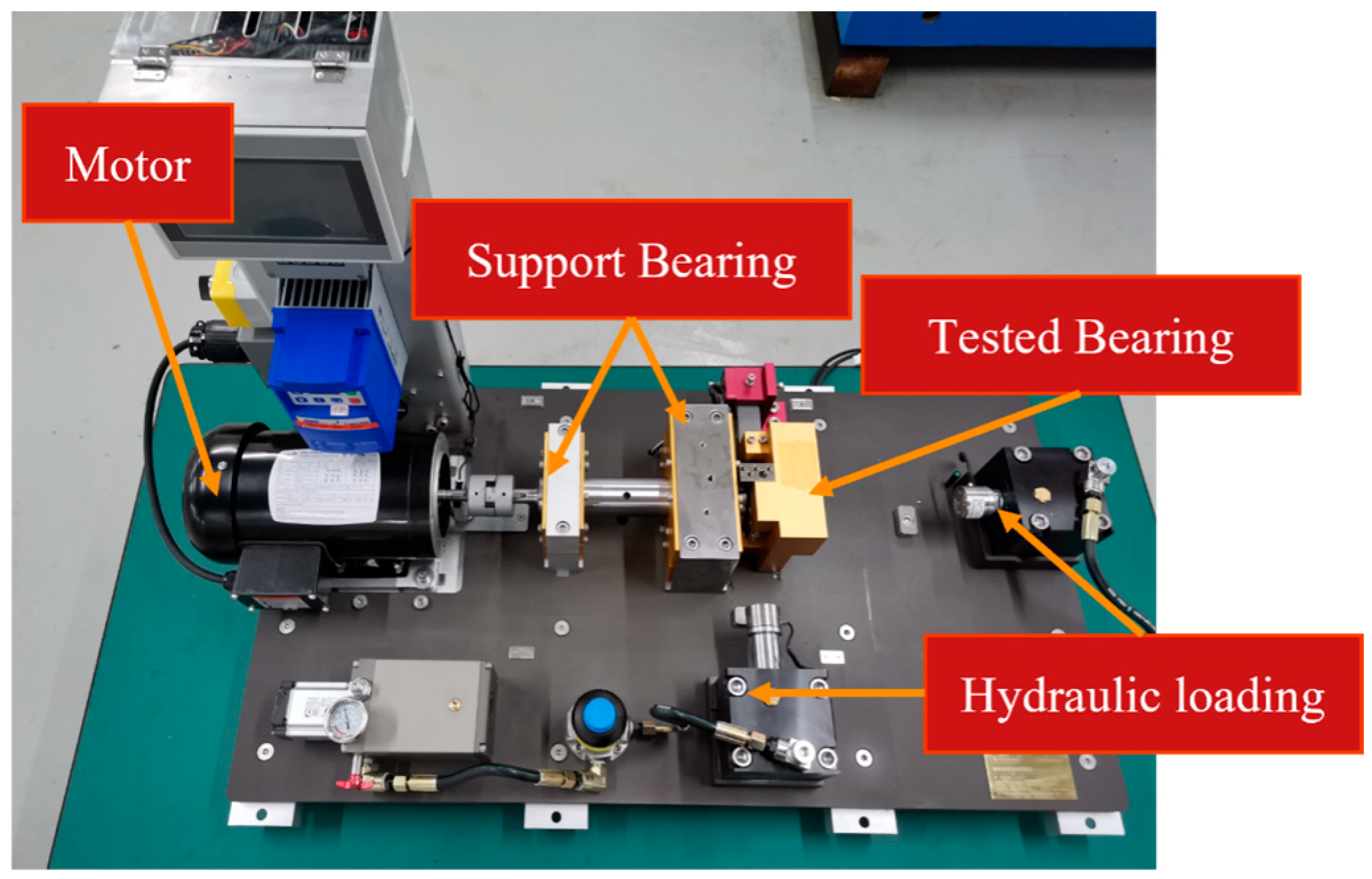
The experimental test bench facility used in this study is available at the Mechanical Engineering Department at Xi’an Jiaotong University, China. The XJTU-SY (Sumyoung Technology-Co, Ltd., Changxing, China.) bearing test rig has a complete suite of features to simulate different conditions and gather many types of data. The experimental test bench is shown in
Figure 1.
For this study, the bearings used are test 16207 and ER-16K. Hydraulic loading blocks are available for axial and radial loading of the test bearing. Vertical and horizontal accelerometers are mounted to the test bearing. Furthermore, acoustic sensors are mounted near the test bearing block. Current sensors are connected to each of the motor phases. A photoelectric tachometer records the key signal and RPM. All of these sensors are connected to the National Instruments card NI 9232. This is connected to a computer system for data acquisition.
Two types of data are required for this diagnostics system. For anomaly detection, progressive degradation data is required. For degradation data, the bearing used RE-16K. A constant radial load of 4 KN and a constant axial load of 0.5 KN are applied to the test bearing. The rotation speed is configured from 10 Hz to 50 Hz every 0.5 h. The sampling frequency is set at 20,480 Hz. A sample is collected every half hour for 3 s. The test was run until failure. The failure mode of the bearing was inner ring failure. In total, 800 samples of data were collected from this experiment.
The fault type data was collected with 16,207 bearings. The bearing was applied with an axial load of 100 KN. Two rotation speeds of 40 Hz and 45 Hz were selected. Data is collected at a sampling frequency of 20,480 Hz. Sample data is collected for 10 s each time. The faults for which the data is collected are cage fault, inner race fault, outer race fault, and rolling-element fault. A total of 200 samples of each fault were collected for each speed.
3. Results and Analysis
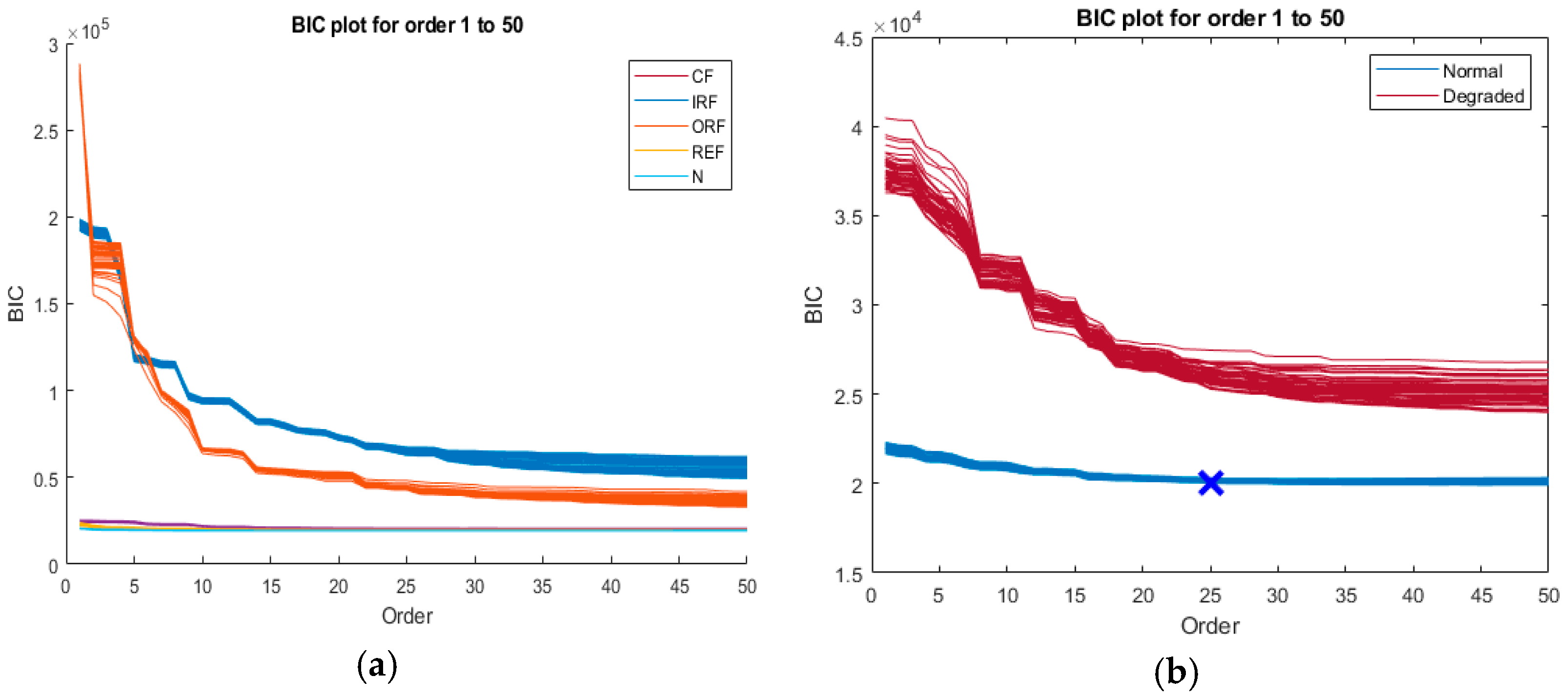
The Bayesian Information Criterion (BIC) is used to find the optimal order of the AR model. The order range was selected to be from 1 to 50 in this case.
Figure 2a shows that the BIC decreases gradually from 1 to 25. Then it starts to increase again very slowly. Thus, a BIC is lowest in the order of 25 in this case.
The order with the lowest BIC will give the AR model with the best feature extraction. It is also important to discuss two groups of curves seen in this plot. The lower group is for normal bearings. It is relatively flat. This means the signals are simple patterns. The second group of curves is for degraded bearing samples. It shows that for lower orders; the BIC is very high. This higher order means that more previous data points are used for modelling the signal. A BIC plot for fault type data is also shown in
Figure 2b. Inner race faults and outer race faults have the largest values for the BIC. These values decrease sharply as order increases progressively. It is of interest to examine the BIC plot in
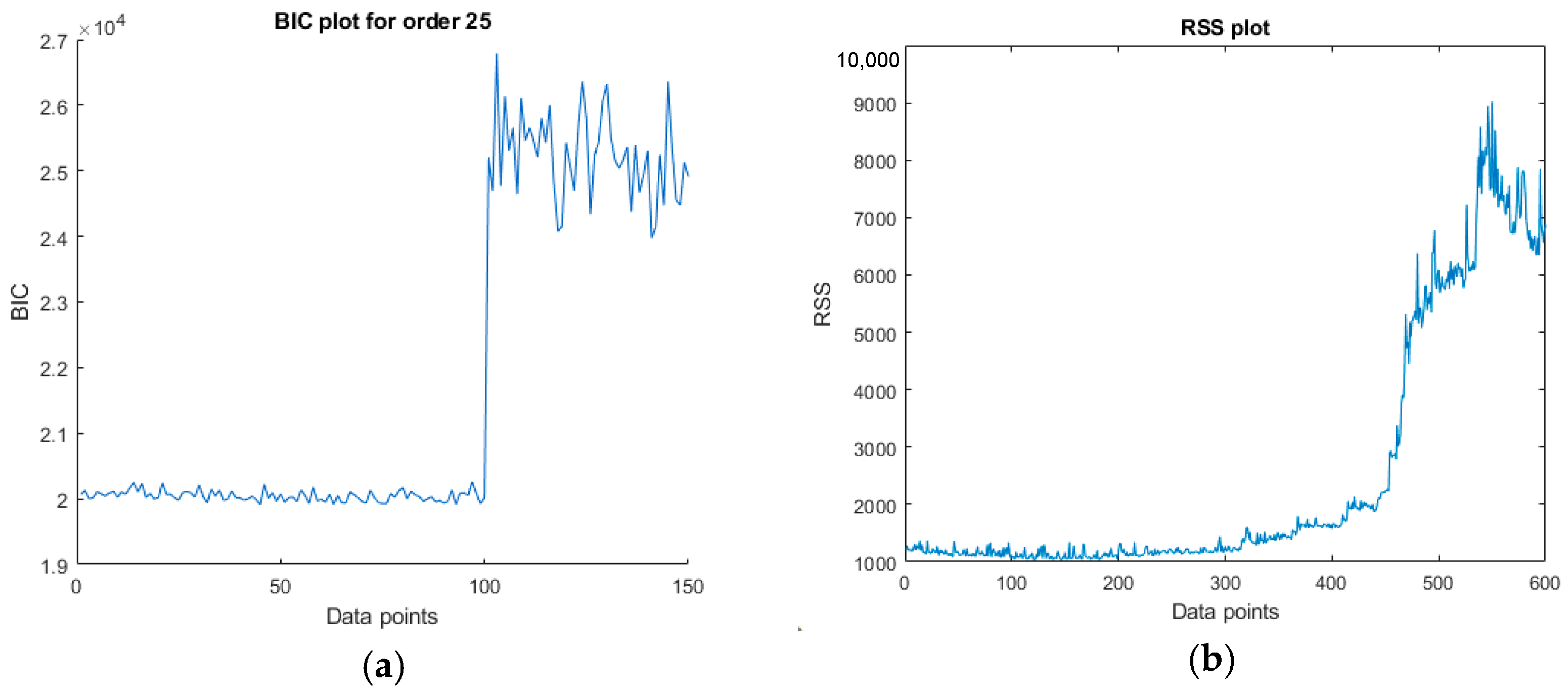
Figure 3 for the data points of a specific order. The plot is shown in
Figure 3a.
The data points up to 100 are healthy data samples. From 100 to 150, the samples are degraded bearing sample data. Thus, the AR model has difficulty in predicting the faulty data. Thus, AR coefficients alone cannot be used for anomaly detection. RSS is a parameter used to reflect error in the prediction and the actual signal. The statement can be confirmed from the RSS plot shown in
Figure 3b. There is a clear change in RSS from normal data from 0 to 400 points and from 500 to 600 points. This feature is important for anomaly detection.
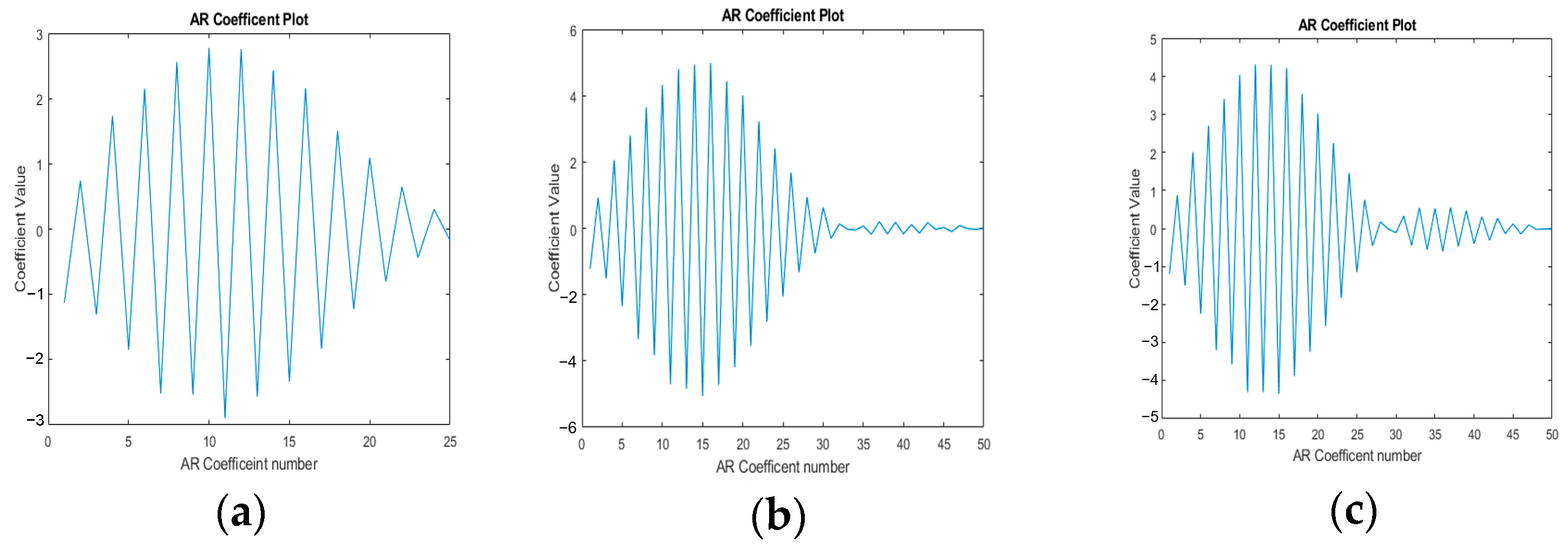
After the order for an AR model, AR coefficients are determined using the Yule–Walker method. The AR coefficient plots against the order are presented in
Figure 4. For this case, the order of 50 is selected for comparison purposes. Since patterns are being extracted from the signal, if the order is sufficiently high, it exhibits a harmonic-like pattern. This is even more deteriorating to the feature extraction process. One such example is shown in
Figure 4c. Thus, proper selection of orders is important and dependent on the data being used.
From
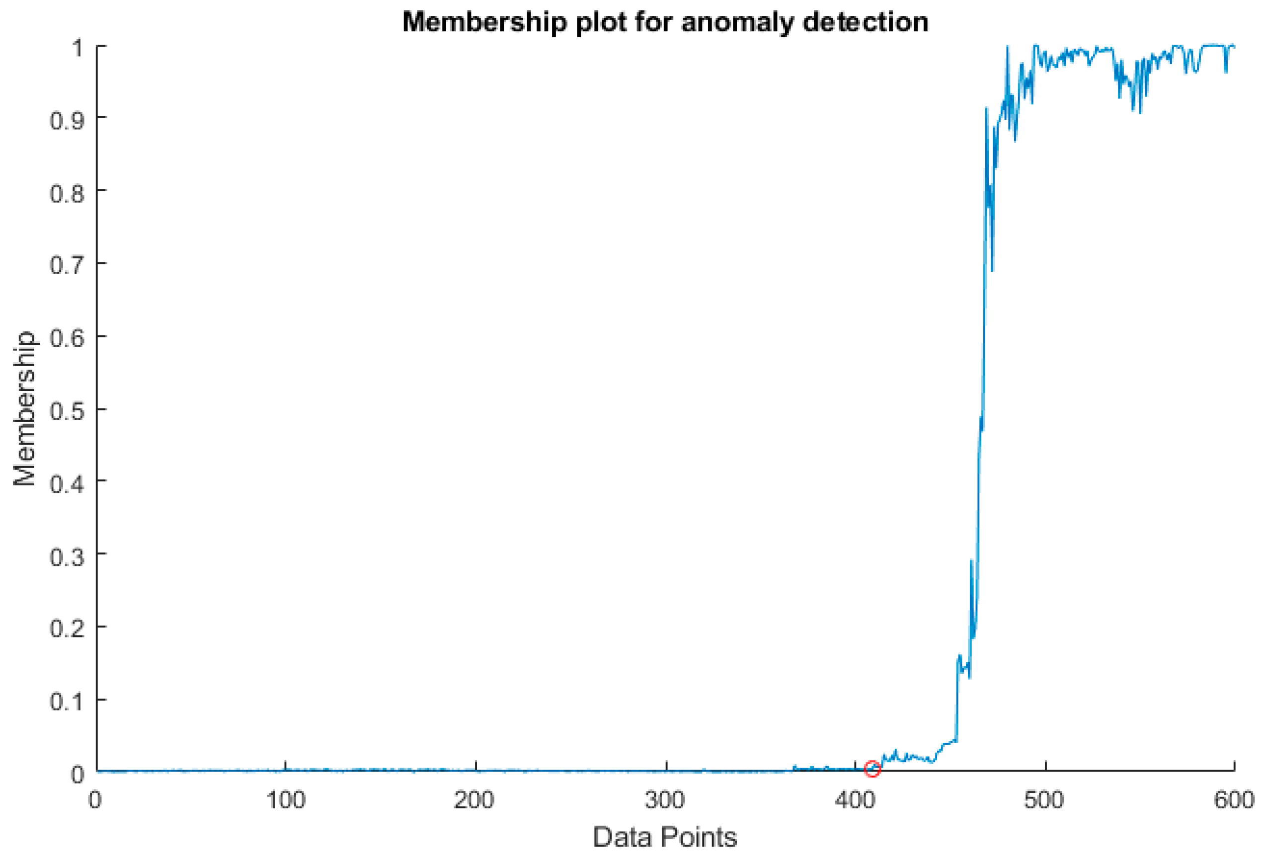
Figure 5, it is evident that after data point 400, clear changes in membership are exhibited.
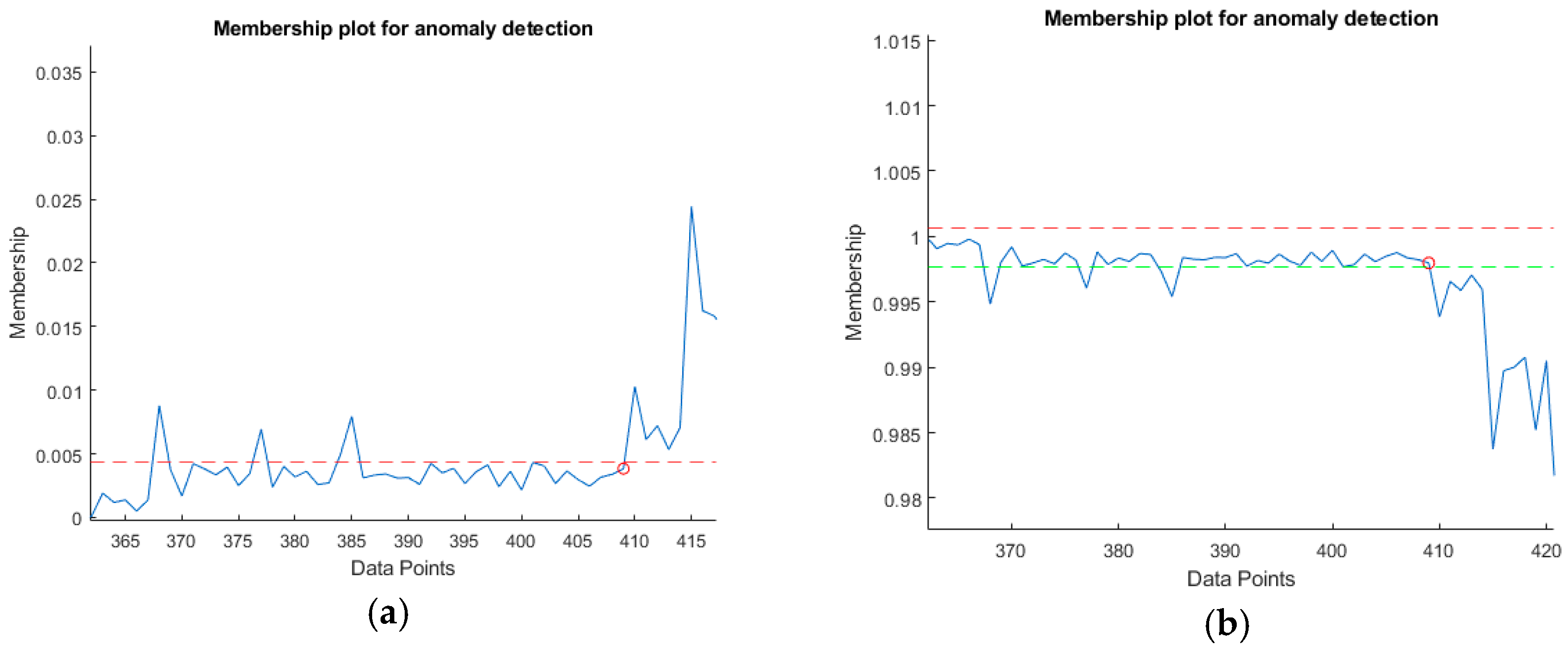
Anomaly detection is performed based on the cluster membership evaluated by the FCM. Three-sigma thresholds are set for the detection.
Figure 6a provides a visual representation of the threshold marked with a dashed red line. For the upper threshold only, anomalies were not detected in some cases as shown in
Figure 6b. All the memberships are below the red dashed line of the upper threshold. The lower threshold is added below, as shown by the green dashed line. In
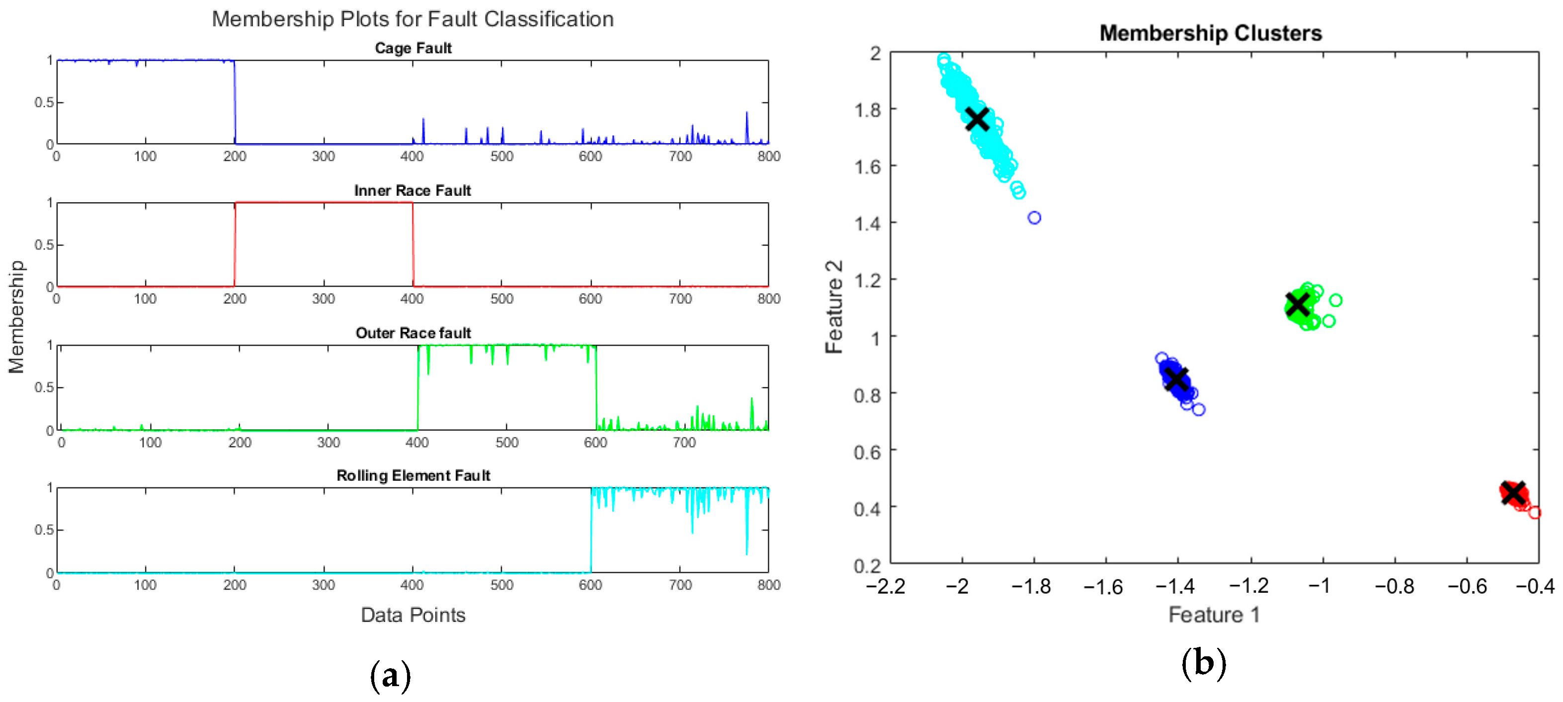
Figure 7, the classification is very good as the faults align well with the separated clusters. The case of rolling-element fault is most difficult to classify. This is most probably due to the absence of dominant unique patterns in the signal.
Table 1 gives a clear look at the performance of FCM training, where one sample from the rolling-element fault was given a wrong classification. Thus, there is one false negative and one false positive each. Errors like these are highlighted in the confusion matrix. The overall accuracy of the model is 97.7%, indicating a high level of accuracy.
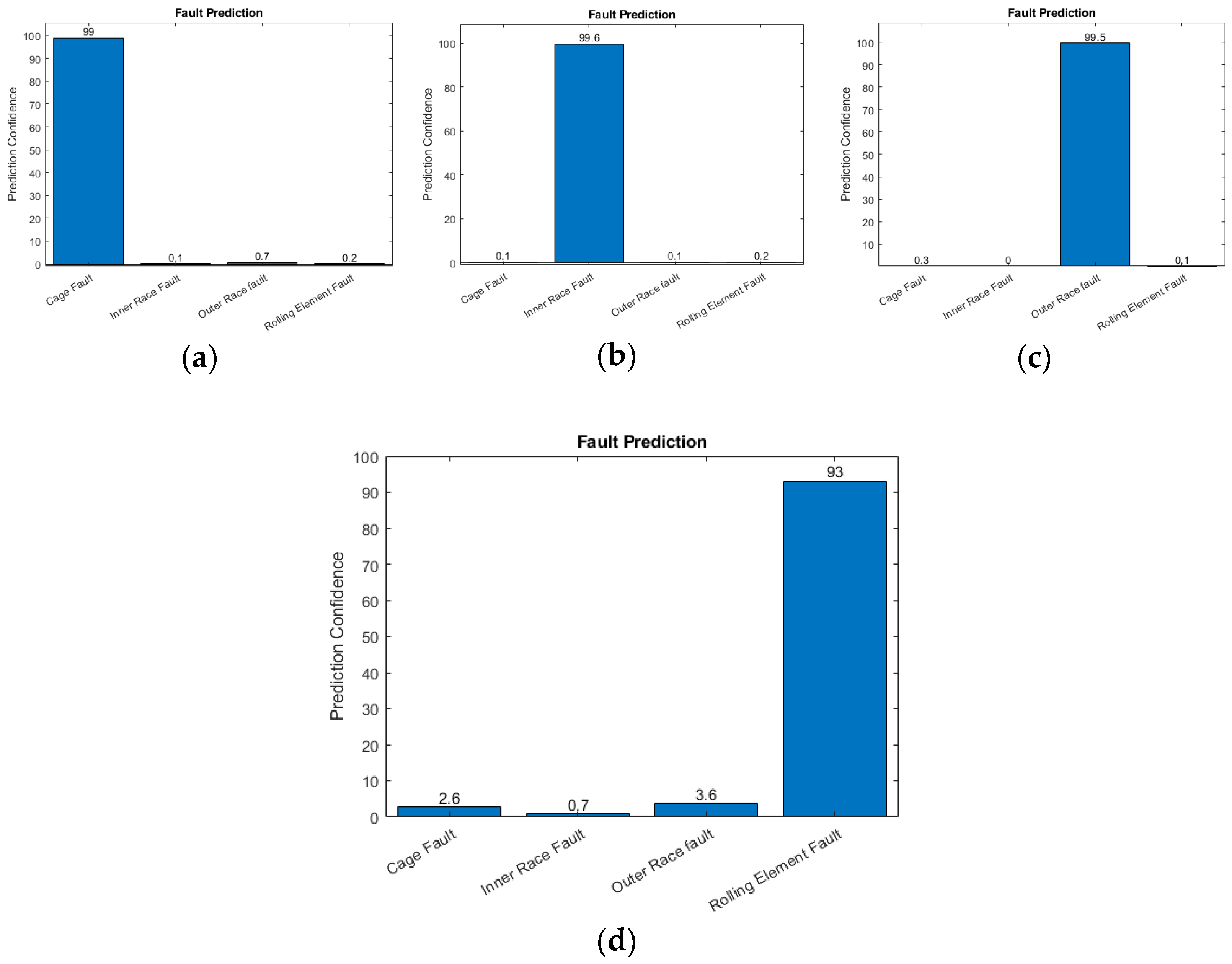
The results from the prediction are shown in
Figure 8. The test sample in (a) is a cage fault, and that in (b) is an inner race fault. The graphs show very high membership of the corresponding faults. This means that the patterns in the sample are correctly extracted and recognized.
Figure 8 shows the other two cases of (c) an outer race fault and (d) a rolling-element fault. It should be noted that the percentage of membership for rolling-element fault is lower by a little bit. This is due to the difficulty of FCM recognizing the pattern.
4. Effect of Fuzziness on Results
4.1. Effect on Anomaly Detection
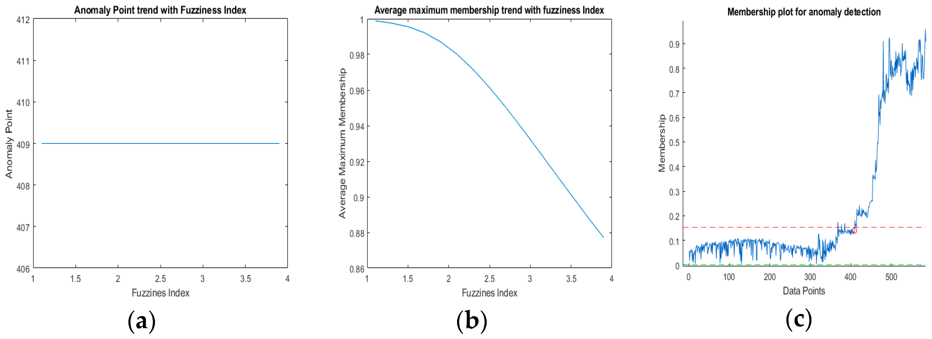
Fuzziness varied in a range between 1.1 and 4.0. The anomaly detection point trend with fuzziness is shown in
Figure 9a. There is no change in anomaly points for the whole range. This is very strange at first. The result shows that fuzziness does not affect the anomaly detection results. The average maximum membership curve with a fuzziness range is shown in
Figure 9b. It can be seen that the average maximum membership decreases progressively. This shows that membership decreases as fuzziness increases.
Figure 9c clearly shows that the membership of points is “fuzzy” compared to
Figure 5, where the fuzziness index was set at 2.0. One more observation to note is that the threshold is also very wide compared to
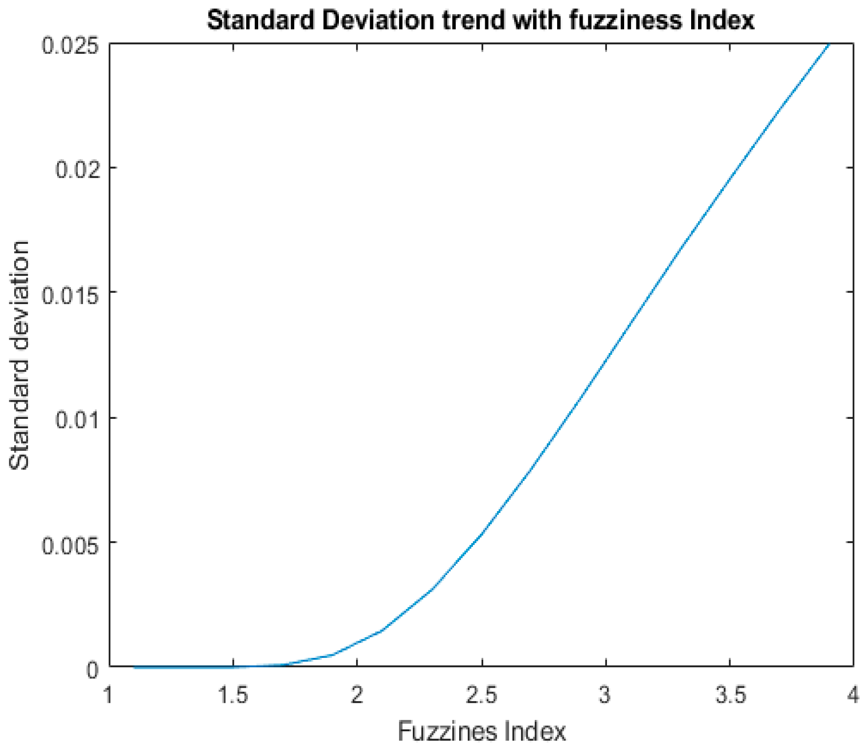
Figure 5. This led to investigating the effect of the fuzziness index on the threshold. In
Figure 10, the effect on the standard deviation increases with fuzziness. This trend is opposite to the average maximum membership trend shown in
Figure 9b. As fuzziness is increased, standard deviation increases. Since the anomaly is detected by the three-sigma rule, the effect of membership decrease is not significant. Thus, we obtain consistent results regardless of the fuzziness index.
4.2. Effect on Fault Classification
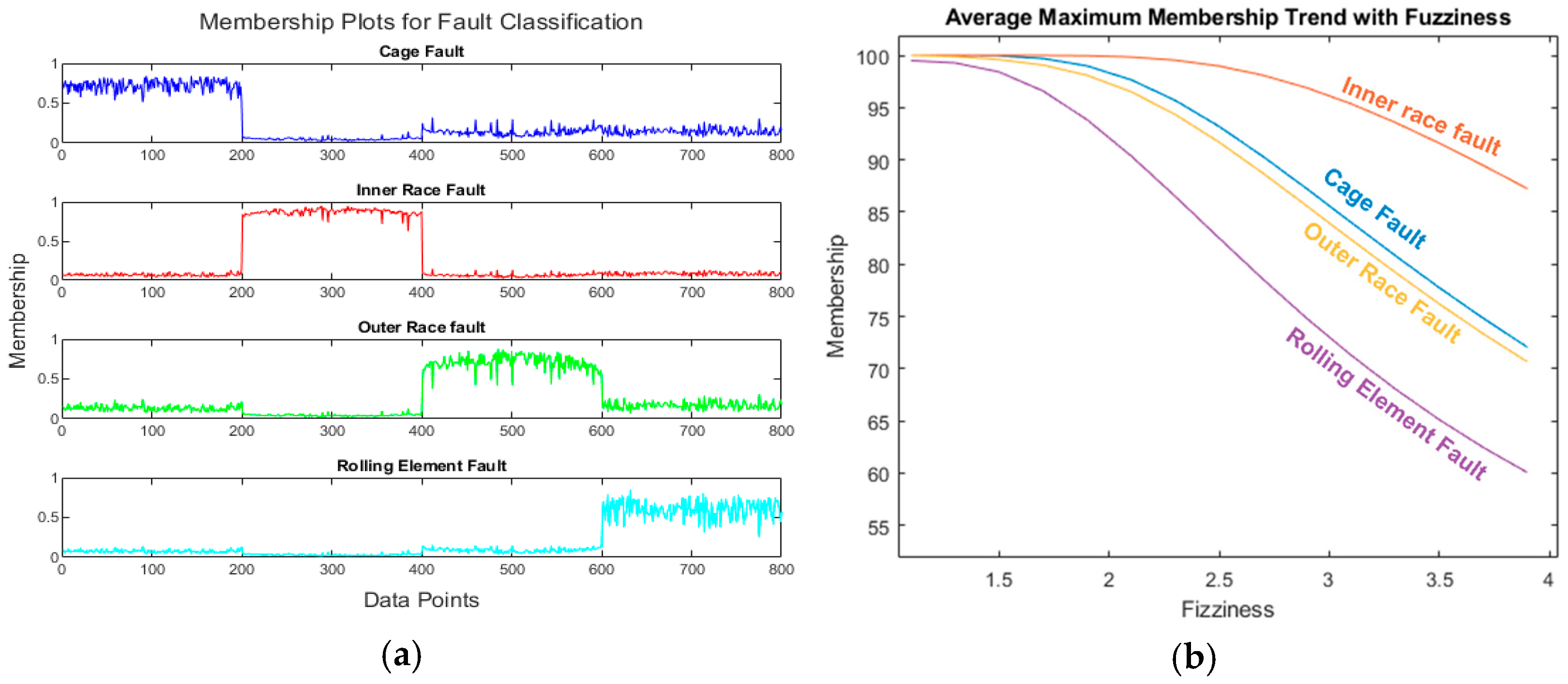
The membership of clusters for a fuzziness index of 3.9 is shown in
Figure 11a. It is clear that the cluster separation is not as clear as that shown in
Figure 7a, where the fuzziness index was set at 2.0. In
Figure 11b, increasing fuzziness does not affect all fault clusters equally. The inner race fault is the least affected by the fuzziness index. Cage faults and outer race faults are affected in a very similar pattern. The most affected fault from fuzziness is the rolling-element fault. The degradation becomes very large after 2.0. The graph in
Figure 11b is smooth for this reason.
5. Effect of Data Size on Order Determination
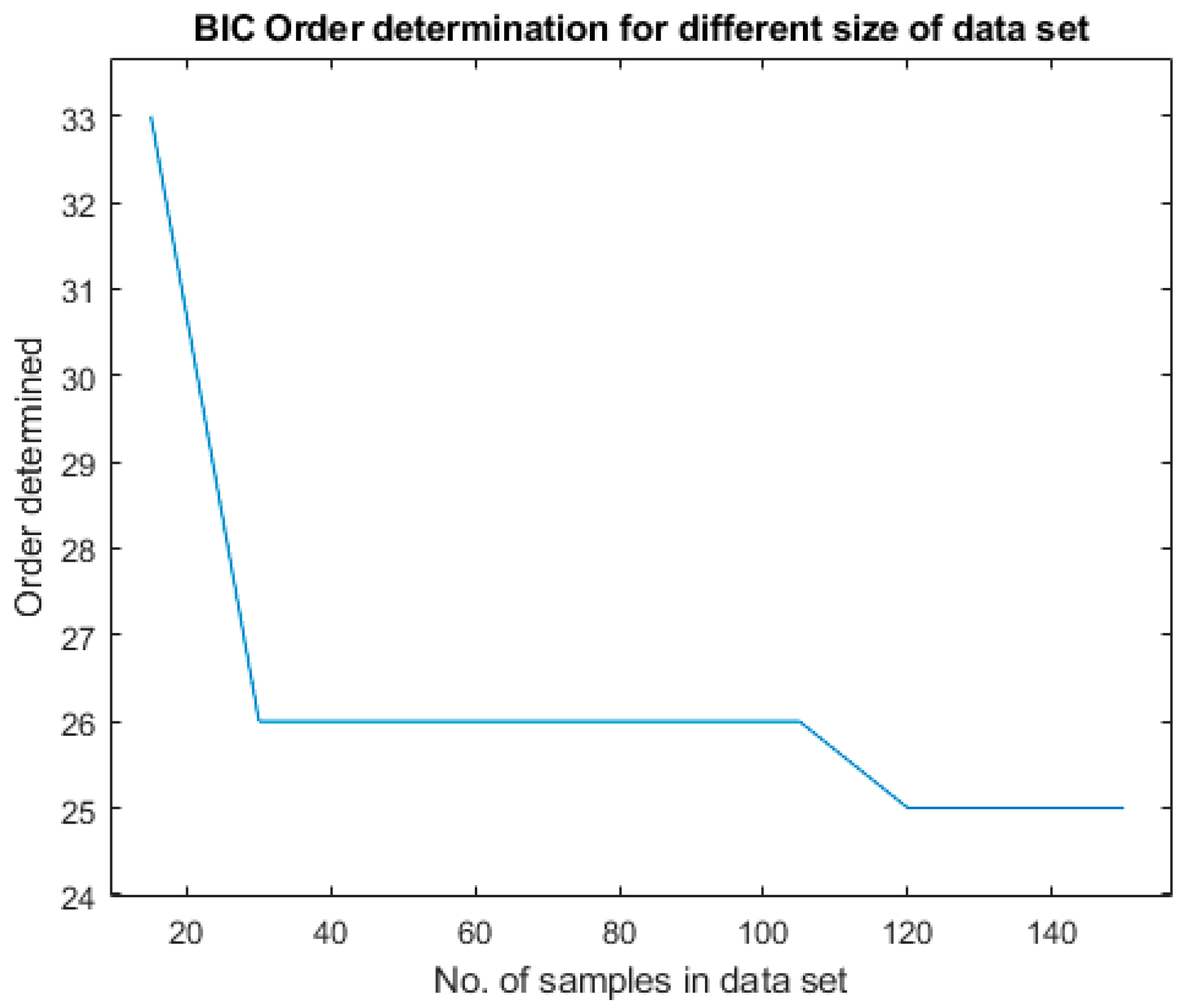
The size of the training set varied from 15 samples (10 normal and 5 degraded) to 150 samples (100 normal and 50 degraded). The result is shown in
Figure 12. For a small data size of 15 samples, the order is determined to be 33. The order is determined to be 26 from a data size of 30 to 115 samples.
6. Effect of Data Size on Fault Classification
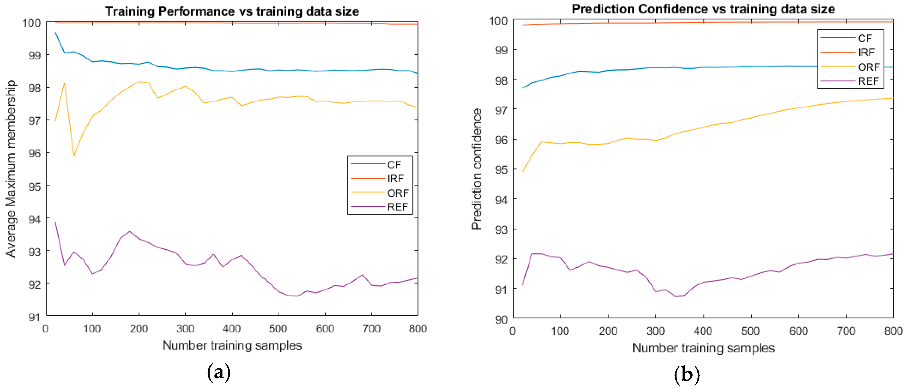
The training data was composed of four faults. Four samples from each fault were combined to form an initial training dataset. The training sample is increased by four samples from each fault. The results are shown in
Figure 13. In part (a), the average maximum membership of the training data is shown. The results show that the effect on each fault is not uniform. Inner race faults show no meaningful differences in prediction and average maximum membership. IRF and ORF show a different pattern. The average maximum membership decreases progressively.
The prediction confidence shows an increase with increasing training dataset samples.
7. Condition Indicators (CIs)
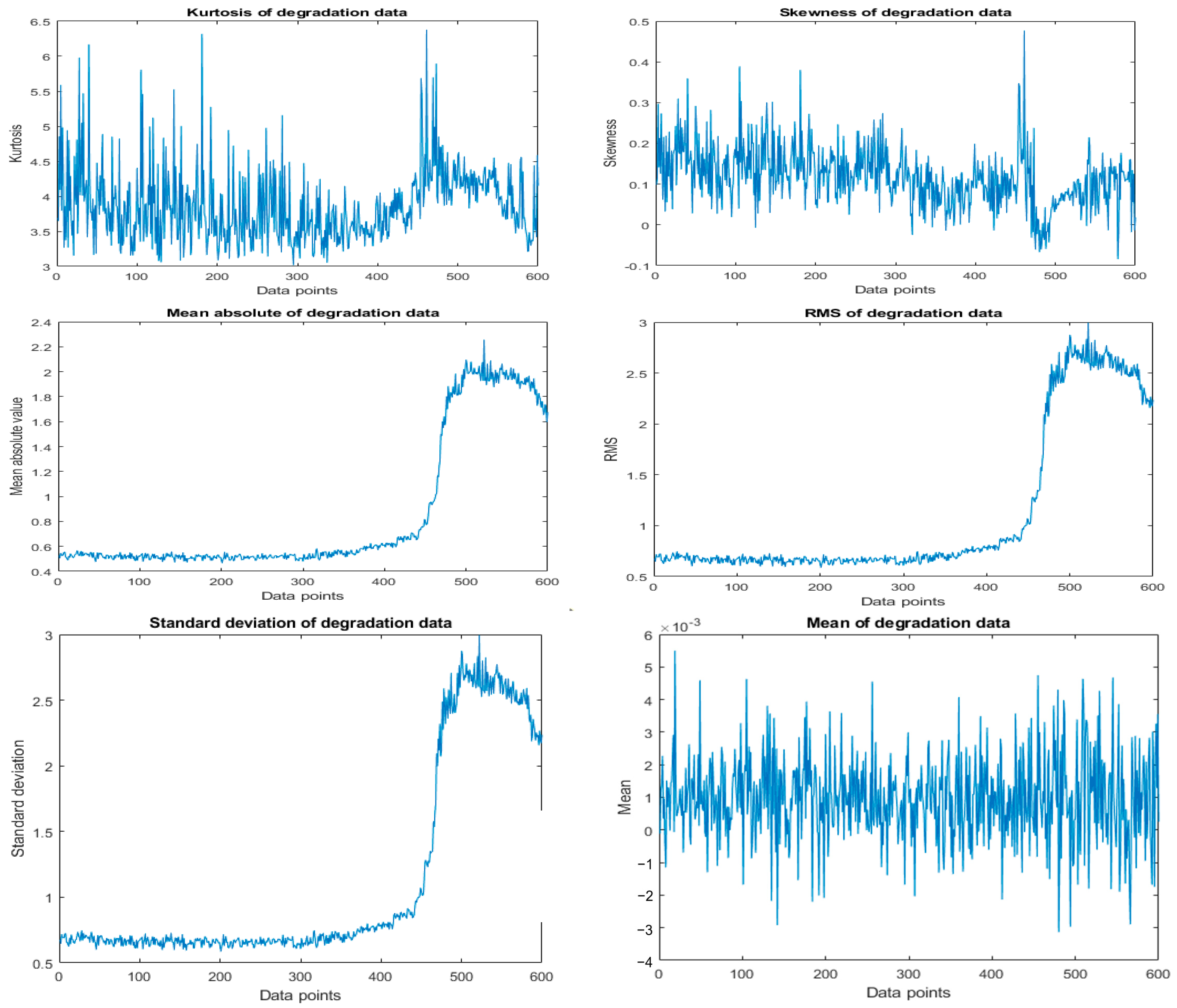
The condition indicator calculations are rather simple. The plots are shown in
Figure 14. A simple visual inspection shows that some indicators perform better at highlighting the degradation of the bearing. Kurtosis, skewness, and mean of the data do not show pronounced effect of degradation.
Fault Type Data CIs
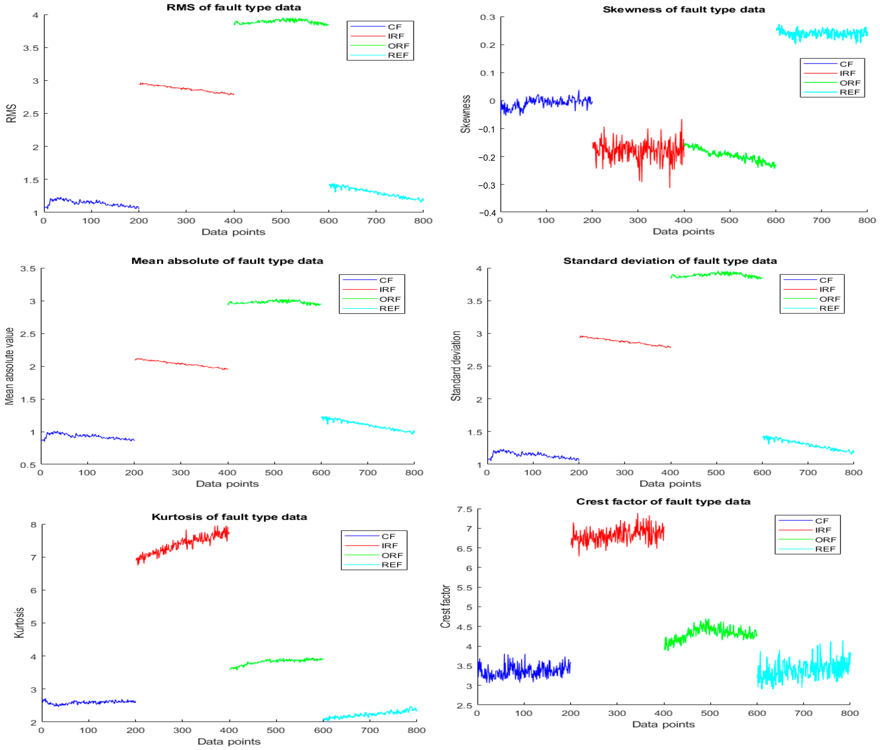
The plots of the condition indicators of the time-domain analysis are shown in
Figure 15.
The case for rolling-element failure shows very similar parameters like cage fault for most of the condition indicators. Skewness is able to separate the rolling-element fault very well. But the inner race fault and outer race fault are not separated well in skewness. One parameter is not sufficient to separate all the faults. AR+FCM extracts these patterns and classifies them according to these factors.
8. Multiple Datasets
To establish robustness and reliability, the system has to be evaluated with data collected from different sources and under different conditions.
For this purpose, additional datasets are utilized. Two speeds of rotation, 40 Hz and 50 Hz, are used to collect data. The average membership of each cluster for each fault is shown in
Figure 16. The rolling-element fault classification accuracy is most affected in all of the datasets.
Effect of Changing Speed on Fault Prediction
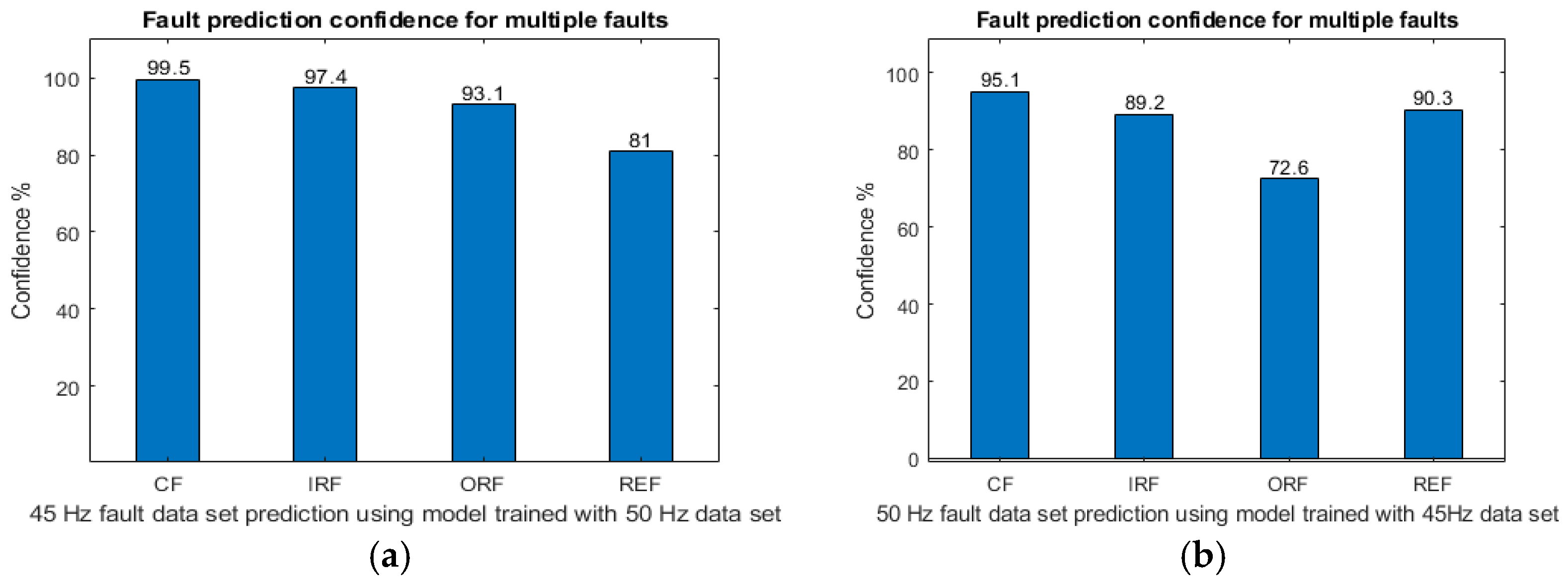
The FCM model is trained using one speed for the dataset. The other dataset with a different speed is then used for fault prediction. The results from the system are then plotted. Rotation speeds of 50 Hz and 45 Hz are used. The results are shown in
Figure 17.
There is some degradation in fault prediction in (a). The case of ORF is most affected by changes in speed. However, (b) shows less of a change in speed.
9. Comparative Analysis
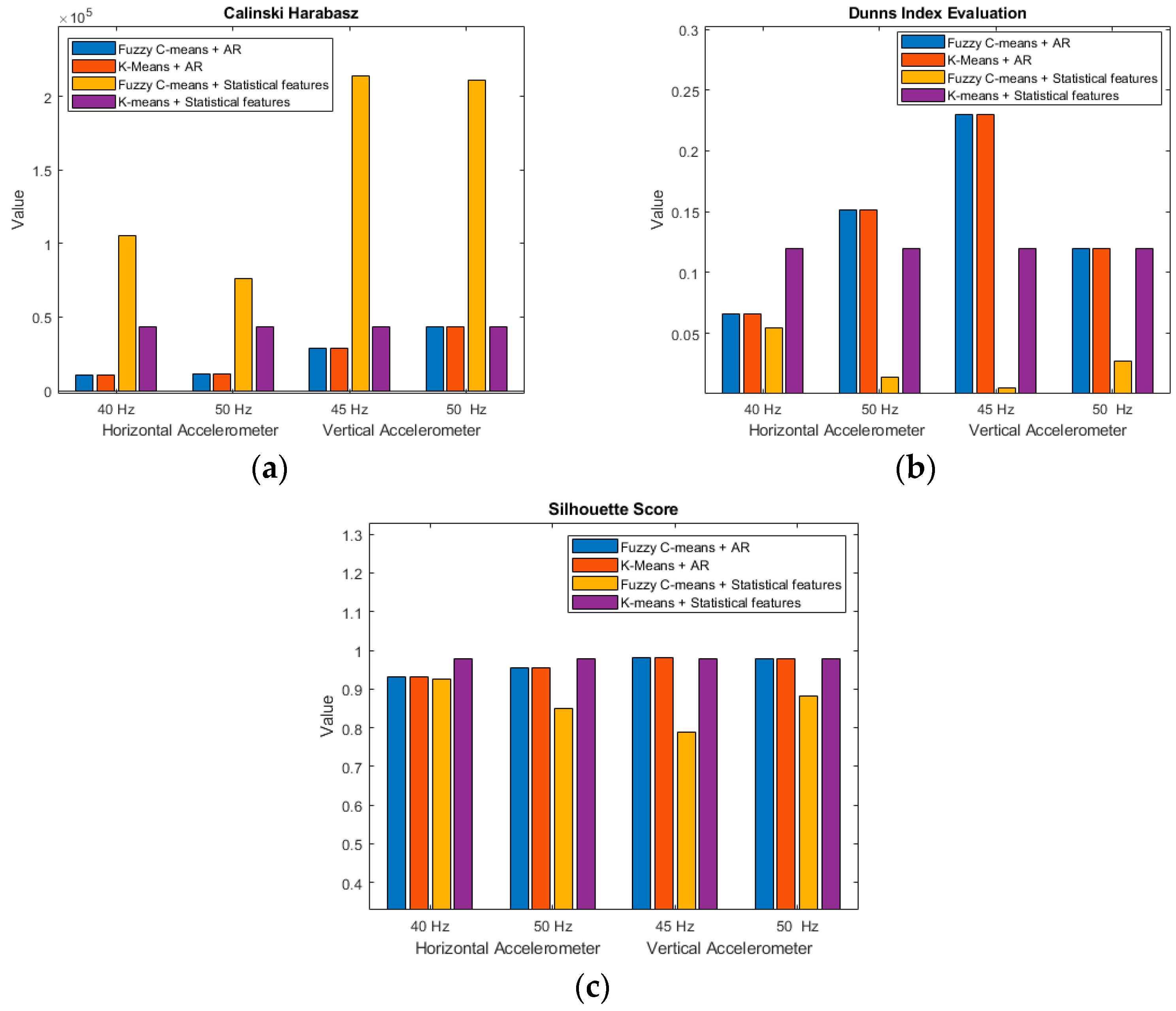
Three indices named the Dunn Index (DI) [
15], the Silhouette Score [
16], and the Calinski–Harabasz index [
17], are calculated. The results are then plotted in the bar graph shown in
Figure 18. The FCM+ statistical features could not provide good classifications. For vertical accelerometers, the Calinski–Harabasz index was able to determine the fault for this particular system. The Silhouette Score and Dunn Index show a clear pattern of the AR+FCM system giving better clustering results. The closest clustering was carried out by the K-means+AR system.
10. Conclusions
This study introduces a simple yet robust predictive methodology for the detection of various faults using bearings by integrating AR-driven feature extraction and FCM classification. After much optimization, the system can achieve an accuracy of almost 97.7%. FCM exhibits a strong performance with varying sensor orientations and rotational speeds. A thorough investigation has been carried out into the parameters of FCM to optimize the results. It was found that training data size and the optimal fuzziness index selection, with lower indices (e.g., 2.0), produce clearer cluster gaps. Comparative analyses demonstrate AR+FCM’s productivity in clustering metrics compared to established approaches. Transient loads and speed variations degrade system performance significantly. Some hybrid models, incorporating deep learning for enhanced feature extraction and testing the system on diverse industrial datasets, can be explored in future studies. Deep learning and advanced analysis techniques require more effort to implement. Better results can be achieved. But the objective of this study was to use fault diagnosis in construction machinery. Applications of advanced techniques are not feasible in the system. A simple robust system is required. Fault classification is carried out mostly by taking samples at steady operating conditions. For performance validation, similar data analysis techniques such as wavelet transform, statistical features, K-Means clustering, etc., have been used. The results show that simplicity and ease of application are still strong points for this technique. The system has unsupervised learning. Labelled data is not required for fault classification. Fault detection can just be trained on normal condition data. This methodology can advance predictive maintenance strategies, making timely predictions to mitigate failures in various machines.
Author Contributions
Conceptualization, W.K. and E.U.; methodology, R.M.A. and E.U.; software, R.M.A.; validation, R.M.A. and E.U. and W.K.; formal analysis, W.K. and E.U.; investigation, R.M.A. and W.K.; resources, R.M.A.; data curation R.M.A. and W.K.; writing—original draft preparation, W.K. and R.M.A.; writing—review and editing, W.K. and E.U.; visualization, R.M.A.; supervision, E.U.; project administration, E.U.; funding acquisition, E.U. All authors have read and agreed to the published version of the manuscript.
Funding
No external funding is acquired for this project.
Institutional Review Board Statement
Not applicable.
Informed Consent Statement
Not applicable.
Data Availability Statement
Data is currently not public due to some privacy concerns but can be made available upon individual request.
Conflicts of Interest
The authors declare no conflict of interest.
References
- Varanis, M.; Silva, A.; Mereles, A.; Pederiva, R. MEMS accelerometers for mechanical vibrations analysis: A comprehensive review with applications. J. Braz. Soc. Mech. Sci. Eng. 2018, 40, 527. [Google Scholar] [CrossRef]
- Randall, R.B.; Antoni, J. Rolling element bearing diagnostics—A tutorial. Mech. Syst. Signal Process. 2011, 25, 485–520. [Google Scholar] [CrossRef]
- Lei, Y.; Lin, J.; He, Z.; Zuo, M.J. A review on empirical mode decomposition in fault diagnosis of rotating machinery. Mech. Syst. Signal Process. 2013, 35, 108–126. [Google Scholar] [CrossRef]
- Ting-Ting, X.; Yan, Z.; Zong, M.; Xiao-Lin, G. A fault diagnosis method of rolling bearing based on VMD Tsallis entropy and FCM clustering. Multimed. Tools Appl. 2020, 79, 30069–30085. [Google Scholar] [CrossRef]
- Lu, W.; Zhang, L.; Liang, W.; Yu, X. A novel feature extraction and optimisation method for fault diagnosis by combining WPT with FCM. Insight Non-Destr. Test Cond. Monit. 2016, 58, 35–41. [Google Scholar] [CrossRef]
- Li, J.; Zhao, R.; Deng, L. Application of EWT AR model and FCM clustering in rolling bearing fault diagnosis. In Proceedings of the 2017 Prognostics and System Health Management Conference (PHM-Harbin), Harbin, China, 9–12 July 2017; pp. 1–6. [Google Scholar]
- Wang, W.; Wong, A.K. Autoregressive Model-Based Gear Fault Diagnosis. J. Vib. Acoust. 2002, 124, 172–179. [Google Scholar] [CrossRef]
- Peng, B.; Bi, Y.; Xue, B.; Zhang, M.; Wan, S. A survey on fault diagnosis of rolling bearings. Algorithms 2022, 15, 347. [Google Scholar] [CrossRef]
- Bauer, M.; Balaratnam, N.; Weidenauer, J.; Wagner, F.; Kley, M. Comparison of envelope demodulation methods in the analysis of rolling bearing damage. J. Vib. Control 2022, 29, 5009–5020. [Google Scholar] [CrossRef]
- Wang, X.; Makis, V. Autoregressive model-based gear shaft fault diagnosis using the Kolmogorov–Smirnov test. J. Sound Vib. 2009, 327, 413–423. [Google Scholar] [CrossRef]
- Altmann, J.; Mathew, J. Multiple band-pass autoregressive demodulation for rolling-element bearing fault diagnosis. Mech. Syst. Signal Process. 2001, 15, 963–977. [Google Scholar] [CrossRef]
- Barbosa, R.; Ferreira, S. Industrial Gas Turbine Diagnostics Using Fuzzy Logic. In Proceedings of the ASME Turbo Expo 2012: Turbine Technical Conference and Exposition, Copenhagen, Denmark, 11–15 June 2012; pp. 803–808. [Google Scholar]
- Pan, Y.; Chen, J.; Li, X. Bearing performance degradation assessment based on lifting wavelet packet decomposition and fuzzy c-means. Mech. Syst. Signal Process. 2010, 24, 559–566. [Google Scholar] [CrossRef]
- Zhao, Q.; Wang, J.; Yin, J.; Zhang, P.; Xie, Z. Peak envelope spectrum Fourier decomposition method and its application in fault diagnosis of rolling bearings. Measurement 2022, 198. [Google Scholar] [CrossRef]
- Dunn, J.C. Well-Separated Clusters and Optimal Fuzzy Partitions. J. Cybern. 1974, 4, 95–104. [Google Scholar] [CrossRef]
- Rousseeuw, P.J. Silhouettes: A graphical aid to the interpretation and validation of cluster analysis. J. Comput. Appl. Math. 1987, 20, 53–65. [Google Scholar] [CrossRef]
- Caliński, T.; Harabasz, J. A dendrite method for cluster analysis. Commun. Stat.-Theory Methods 1974, 3, 1–27. [Google Scholar] [CrossRef]
Figure 1.
XJTU-SU bearing test rig.
Figure 1.
XJTU-SU bearing test rig.
Figure 2.
BIC plots for the order range 1–50: (a) degradation data and (b) fault type data.
Figure 2.
BIC plots for the order range 1–50: (a) degradation data and (b) fault type data.
Figure 3.
(a) BIC for order of 25 calculated for data samples; (b) residual sum of squares (RSS) of the same data.
Figure 3.
(a) BIC for order of 25 calculated for data samples; (b) residual sum of squares (RSS) of the same data.
Figure 4.
AR coefficient for orders of (a) 25 and (b) 50, as well as (c) an anomaly.
Figure 4.
AR coefficient for orders of (a) 25 and (b) 50, as well as (c) an anomaly.
Figure 5.
Clustering for anomaly detection.
Figure 5.
Clustering for anomaly detection.
Figure 6.
Anomaly detection: (a) single-side threshold; (b) threshold range.
Figure 6.
Anomaly detection: (a) single-side threshold; (b) threshold range.
Figure 7.
(a) Membership of the data points for the clusters; (b) clustered data.
Figure 7.
(a) Membership of the data points for the clusters; (b) clustered data.
Figure 8.
Fault prediction of test data: (a) cage fault, (b) inner race fault, (c) outer race fault, and (d) rolling-element fault.
Figure 8.
Fault prediction of test data: (a) cage fault, (b) inner race fault, (c) outer race fault, and (d) rolling-element fault.
Figure 9.
(a) Effect on anomaly point detection by fuzziness index; (b) average maximum membership trend with fuzziness index; and (c) average membership plot at a fuzziness index of 3.9 for anomaly detection.
Figure 9.
(a) Effect on anomaly point detection by fuzziness index; (b) average maximum membership trend with fuzziness index; and (c) average membership plot at a fuzziness index of 3.9 for anomaly detection.
Figure 10.
Standard deviation of membership matrix over range of values for fuzziness index.
Figure 10.
Standard deviation of membership matrix over range of values for fuzziness index.
Figure 11.
(a) Cluster membership plot for a fuzziness index of 3.9; (b) average maximum membership of each cluster trend with fuzziness.
Figure 11.
(a) Cluster membership plot for a fuzziness index of 3.9; (b) average maximum membership of each cluster trend with fuzziness.
Figure 12.
Effect of size of training data on order determination by BIC.
Figure 12.
Effect of size of training data on order determination by BIC.
Figure 13.
Effect on training sample: (a) training performance and (b) prediction confidence.
Figure 13.
Effect on training sample: (a) training performance and (b) prediction confidence.
Figure 14.
Time-domain condition indicators.
Figure 14.
Time-domain condition indicators.
Figure 15.
Condition indicators for fault type data.
Figure 15.
Condition indicators for fault type data.
Figure 16.
Average membership of each cluster for multiple datasets.
Figure 16.
Average membership of each cluster for multiple datasets.
Figure 17.
Fault prediction: (a) 50 Hz dataset using model trained with 45 Hz; (b) 45 Hz using model trained with 50 Hz using horizontal accelerometer data.
Figure 17.
Fault prediction: (a) 50 Hz dataset using model trained with 45 Hz; (b) 45 Hz using model trained with 50 Hz using horizontal accelerometer data.
Figure 18.
(a) Calinski–Harabasz index; (b) Dunn Index; and (c) Silhouette Score.
Figure 18.
(a) Calinski–Harabasz index; (b) Dunn Index; and (c) Silhouette Score.
Table 1.
Confusion matrix for fault classification.
Table 1.
Confusion matrix for fault classification.
| | Actual | Cage Fault | Inner Race Fault | Outer Race Fault | Rolling-Element Fault |
|---|
| Predicted | |
|---|
| Cage Fault, % | 98.98 | 0.01 | 1.5 | 0.1 |
| Inner Race Fault, % | 0.1 | 99.9 | 0.1 | 0.1 |
| Outer Race Fault, % | 1.5 | 0.01 | 98.1 | 0.3 |
| Rolling-Element Fault, % | 2.4 | 0.01 | 3.48 | 93.8 |
| Disclaimer/Publisher’s Note: The statements, opinions and data contained in all publications are solely those of the individual author(s) and contributor(s) and not of MDPI and/or the editor(s). MDPI and/or the editor(s) disclaim responsibility for any injury to people or property resulting from any ideas, methods, instructions or products referred to in the content. |
© 2025 by the authors. Licensee MDPI, Basel, Switzerland. This article is an open access article distributed under the terms and conditions of the Creative Commons Attribution (CC BY) license (https://creativecommons.org/licenses/by/4.0/).
