Case Study of Binary Hypothesis Test Using ML ^†

Abstract

Artificial intelligence has attracted much attention due to its learning capability to solve versatile problems. Using a convolutional neural network in machine learning (ML), we investigated the binary hypothesis test, which is a fundamental problem in management and business. The simulation results showed that the proposed method is comparable with the conventional optimum likelihood ratio test for the aspect of type I and II errors. Moreover, the learning capability of ML is promising for complicated data, the properties of which, such as probability distribution and/or statistical data, i.e., mean, variance, and others, are not known.

1. Introduction

The binary hypothesis test is used to select better hypotheses between ${\mathcal{H}}_0$ and ${\mathcal{H}}_1$ infers based on measurement data. Many applications are used in management and business [1,2], communications [3,4], and biology [5,6,7]. The hypothesis test enables the analysis and evaluation of the causes and effects of important management decisions. Using the hypothesis test, data-driven decision-makers translate data into their business strategy.

Traditionally, the hypothesis test is conducted using the Bayesian approach. Recently, machine learning (ML) has attracted considerable attention due to its outstanding classification capability using features embedded in observed data. Characterized by the use of data and algorithms, ML is used to solve problems by imitating the way that humans learn and improve their performance (or intelligence). Convolutional neural networks (CNNs) [8,9] are popular deep learning technologies that are often used in image or speech recognition, object detection, and other fields. Compared with the traditional multilayer perceptron (MLP), the CNN introduces the concept of windows. This allows the CNN to effectively capture high-level features of the data observed through these windows. CNNs usually contain various layers, such as convolutional layers, activation functions, pooling layers, and fully connected layers [8].

In contrast to the conventional likelihood ratio test, we studied the binary hypothesis test using the ML approach. Using the CNN, a solution was proposed, and the results were compared with that of the optimum likelihood ratio test in this study. Consequently, the learning capability of CNN models is promising for solving the considered problem of binary hypothesis tests in wide applications.

The rest of this article is organized as follows. Section 2 introduces the problem. Section 3 presents two case studies employing the conventional likelihood ratio test. Section 4 introduces the proposed CNN scheme, and Section 5 demonstrates simulation results and concludes this study.

2. Problem Formulation

Without a loss of generality, the binary hypothesis test was investigated, assuming that data were sampled from the stationary Gaussian random process. Therefore, the joint probability density function (PDF) of N data samples x = ${\left[x_0,x_1\dots x_{N-1}\right]}^T$ under hypothesis ${\mathcal{H}}_i$, I = 0, 1, was expressed as follows:

$$f\left(\mathbf{x}|{\mathcal{H}}_i\right)=\prod _{n=0}^{N-1}{\displaystyle \frac{\mathrm{e}\mathrm{x}\mathrm{p}\left(-\frac{1}{2}{\left(\frac{x_n-{\mu }_i}{{\sigma }_i}\right)}^2\right)}{{\sigma }_i\sqrt{2\pi }}}$$

(1)

where $x_n$ denotes data samples; n = 0, 1, …, N − 1; $\prod$ denotes the product operation; ${\mu }_i$ and ${\sigma }_i$ denote the mean and standard deviation of $x_n$ under hypothesis ${\mathcal{H}}_i$, respectively; and ${\mu }_1>{\mu }_0$. Given the data samples, the true hypothesis must be selected. That is, based on x and its joint PDF(1), the most probable hypothesis is inferred as follows:

$$\left\{\begin{array}{c}{\mathcal{H}}_0:\mathbf{x}~f\left(\mathbf{x}|{\mathcal{H}}_0\right)\\ {\mathcal{H}}_1:\mathbf{x}~f\left(\mathbf{x}|{\mathcal{H}}_1\right)\end{array}\right..$$

(2)

3. Case Study Using Likelihood Ratio Test

We explored two cases using the likelihood ratio test.

3.1. Case A: Different Mean with Same Variance

Since mean and variance are basic statistics of Gaussian random variables, their effects on the considered problem were studied. First, we investigated a simple condition with a different mean and the same variance, i.e., ${\mu }_0\ne {\mu }_1$ (${\mu }_1>{\mu }_0$) and ${\sigma }_0^2={\sigma }_1^2$. According to the likelihood ratio test,

$$f(\mathrm{x}|{\mathcal{H}}_1)\begin{array}{c}{\mathcal{H}}_1\\ \gtrless \\ {\mathcal{H}}_0\end{array}f(\mathrm{x}|{\mathcal{H}}_0)$$

(3)

After several manipulations, Equation (4) was used.

$${\displaystyle \frac{1}{N}}\sum _{n=0}^{N-1}{x}_n\begin{array}{c}{\mathcal{H}}_1\\ \gtrless \\ {\mathcal{H}}_0\end{array}{\eta }_A$$

(4)

where ${\eta }_A={\displaystyle \frac{{\mu }_0+{\mu }_1}{2}}$.

The decision metrics (Equation (4)) are comprehensive. When the average value of x is less than ${\eta }_A$ (or the average value of means ${\mu }_0$ and ${\mu }_1$), ${\mathcal{H}}_0$ is decided; otherwise, ${\mathcal{H}}_1$ is inferred.

Under ${\mathcal{H}}_0$ (i.e., $x_n~\aleph \left({\mu }_0,{\sigma }_0^2\right)$, $\forall n$), let $y_A\equiv {\displaystyle \frac{1}{N}}\sum _{n=0}^{N-1}{x}_n$; one has $y_A~\aleph \left({\mu }_{y_A},{\sigma }_{y_A}^2\right)$, where $\aleph \left(·\right)$ denotes the PDF of a Gaussian random variable, ${\mu }_{y_A}{=\mu }_0$ is the mean of $y_A$, and ${\sigma }_{y_A}^2={\sigma }_0^2/N$ is the variance of $y_A$. Therefore, the type I error of case A, ${\alpha }_A$, can be subsequently written as follows:

$$\begin{array}{cc}\hfill {\alpha }_A& =\mathrm{P}\mathrm{r}\mathrm{o}\mathrm{b}\left(y_A>{\eta }_A\right)\hfill \\ & ={\int }_{{\eta }_A}^{\infty }\frac{\mathrm{e}\mathrm{x}\mathrm{p}\left(-\frac{1}{2}{\left(\frac{y_A-{\mu }_{y_A}}{{\sigma }_{y_A}}\right)}^2\right)}{{\sigma }_{y_A}\sqrt{2\pi }}d{y}_A\hfill \end{array}$$

(5)

where $\mathrm{P}\mathrm{r}\mathrm{o}\mathrm{b}\left(·\right)$ denotes the probability.

Apparently, ${\alpha }_A$ does not have the closed-form expression. However, since $z_A={\displaystyle \frac{y_A-{\mu }_{y_A}}{{\sigma }_{y_A}}}$ has the standard normal distribution, ${\alpha }_A$ is rewritten as follows:

$$\begin{array}{cc}\hfill {\alpha }_A& =\mathrm{P}\mathrm{r}\mathrm{o}\mathrm{b}\left({\displaystyle \frac{y_A-{\mu }_{y_A}}{{\sigma }_{y_A}}}>{\displaystyle \frac{{\eta }_A-{\mu }_{y_A}}{{\sigma }_{y_A}}}\right)\hfill \\ & =Q\left({\displaystyle \frac{{\eta }_A-{\mu }_{y_A}}{{\sigma }_{y_A}}}\right),\hfill \end{array}$$

(6)

where $Q\left(·\right)$ denotes the Q function, i.e.,

$$Q\left(x\right)={\int }_x^{\infty }{\displaystyle \frac{\mathrm{e}\mathrm{x}\mathrm{p}\left(-\frac{1}{2}{u}^2\right)}{\sqrt{2\pi }}}du.$$

(7)

Under ${\mathcal{H}}_1$ (i.e., $x_n~\aleph \left({\mu }_1,{\sigma }_1^2\right)$, $\forall n$), let $y_A\equiv {\displaystyle \frac{1}{N}}\sum _{n=0}^{N-1}{x}_n$; one has $y_A~\aleph \left({\mu }_{y_A},{\sigma }_{y_A}^2\right)$, where $\aleph \left(·\right)$ denotes the PDF of a Gaussian random variable, ${\mu }_{y_A}{=\mu }_1$ is the mean of $y_A$, and ${\sigma }_{y_A}^2={\sigma }_1^2/N$ is the variance of $y_A$. Therefore, the type II error of case A, ${\beta }_A$, can be subsequently written as follows:

$$\begin{array}{cc}\hfill {\beta }_A& =\mathrm{P}\mathrm{r}\mathrm{o}\mathrm{b}\left(y_A<{\eta }_A\right)\hfill \\ & ={\int }_{-\infty }^{\frac{{\eta }_A-{\mu }_{y_A}}{{\sigma }_{y_A}}}{\displaystyle \frac{\mathrm{e}\mathrm{x}\mathrm{p}\left(-\frac{1}{2}{z}_A^2\right)}{\sqrt{2\pi }}}d{z}_A\hfill \end{array}$$

(8)

where $z_A={\displaystyle \frac{y_A-{\mu }_{y_A}}{{\sigma }_{y_A}}}$. Let $w_A={-z}_A$:

$$\begin{array}{cc}\hfill {\beta }_A& ={\int }_{-\frac{{\eta }_A-{\mu }_{y_A}}{{\sigma }_{y_A}}}^{\infty }{\displaystyle \frac{\mathrm{e}\mathrm{x}\mathrm{p}\left(-\frac{1}{2}{w}_A^2\right)}{\sqrt{2\pi }}}d{w}_A\hfill \\ & =Q\left(-{\displaystyle \frac{{\eta }_A-{\mu }_{y_A}}{{\sigma }_{y_A}}}\right).\hfill \end{array}$$

(9)

3.2. Case B: Different Mean with Different Variance

In this general case, ${\mu }_0\ne {\mu }_1$ (${\mu }_1>{\mu }_0$) and ${\sigma }_0^2\ne {\sigma }_1^2$. According to the likelihood ratio test (Equation (3)), after several manipulations, the following is derived:

$$\sum _{n=0}^{N-1}{\left({\displaystyle \frac{x_n-{\mu }_0}{{\sigma }_0}}\right)}^2-\sum _{n=0}^{N-1}{\left({\displaystyle \frac{x_n-{\mu }_1}{{\sigma }_1}}\right)}^2\begin{array}{c}{\mathcal{H}}_1\\ \gtrless \\ {\mathcal{H}}_0\end{array}{\eta }_B$$

(10)

where ${\eta }_B=2N\mathrm{l}\mathrm{n}{\displaystyle \frac{{\sigma }_1}{{\sigma }_0}}$ and $\mathrm{l}\mathrm{n}\left(·\right)$ denote the natural logarithm function.

Even though the decision metric (Equation (10)) is not concise, it is enough to be used as the algorithm of the likelihood ratio test for case B. Since the exact distributions of the decision metric under both hypotheses are involved, we derived their asymptotical expressions when N was large. Hence, under ${\mathcal{H}}_0$ (i.e., $x_n~\aleph \left({\mu }_0,{\sigma }_0^2\right)$, $\forall n$), let $y_B\equiv \sum _{n=0}^{N-1}{\left({\displaystyle \frac{x_n-{\mu }_0}{{\sigma }_0}}\right)}^2$ and $w_B\equiv \sum _{n=0}^{N-1}{\left({\displaystyle \frac{x_n-{\mu }_1}{{\sigma }_1}}\right)}^2$; according to the central limit theorem, one has $y_B~\aleph \left({\mu }_{y_B},{\sigma }_{y_B}^2\right)$ and $w_B~\aleph \left({\mu }_{w_B},{\sigma }_{w_B}^2\right)$, where ${\mu }_{y_B}=N$, ${\sigma }_{y_B}^2=2N$, ${\mu }_{w_B}=N{\displaystyle \frac{{\sigma }_0^2}{{\sigma }_1^2}}+N{\displaystyle \frac{{\left({\mu }_0-{\mu }_1\right)}^2}{{\sigma }_1^2}}$, ${\sigma }_{w_B}^2=2N{\displaystyle \frac{{\sigma }_0^4}{{\sigma }_1^4}}+4N{\left({\mu }_0-{\mu }_1\right)}^2{\displaystyle \frac{{\sigma }_0^2}{{\sigma }_1^4}}$ (Appendix A).

Let ${z_B=y}_B-w_B$, then $z_B~\mathrm{\aleph }\left({\mu }_{z_B},{\sigma }_{z_B}^2\right)$, where ${\mu }_{z_B}=N\left(1-{\displaystyle \frac{{\sigma }_0^2}{{\sigma }_1^2}}\right)-N{\displaystyle \frac{{\left({\mu }_0-{\mu }_1\right)}^2}{{\sigma }_1^2}}$ and ${\sigma }_{z_B}^2=2N+2N{\displaystyle \frac{{\sigma }_0^4}{{\sigma }_1^4}}+4N{\left({\mu }_0-{\mu }_1\right)}^2{\displaystyle \frac{{\sigma }_0^2}{{\sigma }_1^4}}-4N{\displaystyle \frac{{\sigma }_0^2}{{\sigma }_1^2}}$ (Appendix B). Therefore, the type I error of case B, ${\alpha }_B$, is written as follows:

$$\begin{array}{cc}\hfill {\alpha }_B& =\mathrm{P}\mathrm{r}\mathrm{o}\mathrm{b}\left(z_B>{\eta }_B\right)\hfill \\ & =Q\left({\displaystyle \frac{{\eta }_B-{\mu }_{z_B}}{{\sigma }_{z_B}}}\right).\hfill \end{array}$$

(11)

Under ${\mathcal{H}}_1$ (i.e., $x_n~\mathrm{\aleph }\left({\mu }_1,{\sigma }_1^2\right)$, $\forall n$), the statistics of $y_B=\sum _{n=0}^{N-1}{\left({\displaystyle \frac{x_n-{\mu }_0}{{\sigma }_0}}\right)}^2$ and $w_B\equiv \sum _{n=0}^{N-1}{\left({\displaystyle \frac{x_n-{\mu }_1}{{\sigma }_1}}\right)}^2$ are similar to $y_B~\mathrm{\aleph }\left({\mu }_{y_B},{\sigma }_{y_B}^2\right)$ and $w_B~\mathrm{\aleph }\left({\mu }_{w_B},{\sigma }_{w_B}^2\right)$, where ${\mu }_{y_B}=N{\displaystyle \frac{{\sigma }_1^2}{{\sigma }_0^2}}+N{\displaystyle \frac{{\left({\mu }_1-{\mu }_0\right)}^2}{{\sigma }_0^2}}$, ${\sigma }_{y_B}^2=2N{\displaystyle \frac{{\sigma }_1^4}{{\sigma }_0^4}}+4N{\left({\mu }_1-{\mu }_0\right)}^2{\displaystyle \frac{{\sigma }_1^2}{{\sigma }_0^4}}$, ${\mu }_{w_B}=N$, and ${\sigma }_{w_B}^2=2N$. Additionally, let ${z_B=y}_B-w_B$, then $z_B~\mathrm{\aleph }\left({\mu }_{z_B},{\sigma }_{z_B}^2\right)$, where ${\mu }_{z_B}=N\left({\displaystyle \frac{{\sigma }_1^2}{{\sigma }_0^2}}-1\right)+N{\displaystyle \frac{{\left({\mu }_1-{\mu }_0\right)}^2}{{\sigma }_0^2}}$ and ${\sigma }_{z_B}^2=2N+2N{\displaystyle \frac{{\sigma }_1^4}{{\sigma }_0^4}}+4N{\left({\mu }_1-{\mu }_0\right)}^2{\displaystyle \frac{{\sigma }_1^2}{{\sigma }_0^4}}-4N{\displaystyle \frac{{\sigma }_1^2}{{\sigma }_0^2}}$. Therefore, the type II error of case B, ${\beta }_B$, can be written as follows:

$${\beta }_B=\mathrm{P}\mathrm{r}\mathrm{o}\mathrm{b}\left(z_B<{\eta }_B\right)=Q\left(-{\displaystyle \frac{{\eta }_B-{\mu }_{z_B}}{{\sigma }_{z_B}}}\right).$$

(12)

4. Proposed ML Based on CNN

Table 1. CNN-based binary hypothesis test with N = 40.

Layer	Output Dimensions	Parameter Number
Input	(40, 1)	0
Convolution	(40, 50)	950
		37,550
		30,050
		22,550
		15,050
		7550
Fully connected	64	128,064
	32	2080
	16	528
	8	136
	1	9

presents the proposed CNN structure for the considered hypothesis test with N = 40. The stride and activation functions of the CNN are one and ReLU, respectively. Compared with the conventional optimum likelihood ratio test, the probability distribution and/or statistical properties of the data samples are not required by CNNs. However, training data and their correct classifications (or labels) are necessary for the ML.

5. Discussion and Conclusions

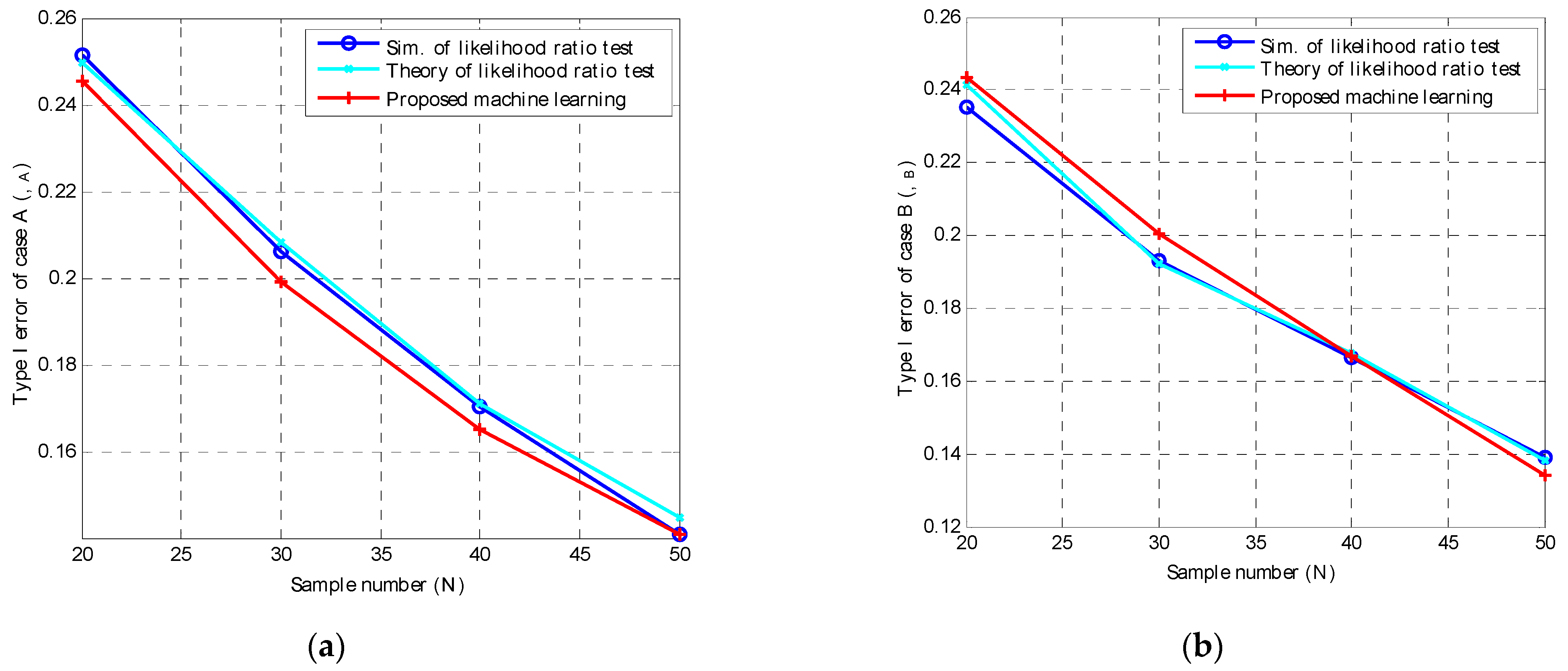
Monte Carlo simulations were used to assess the performance of binary hypothesis tests using different approaches in this study. For case A, 20,000 sets of input data were evenly sampled from the Gaussian random variables with $\left({\mu }_0,{\sigma }_0^2\right)=(-0.15,1)$ and $\left({\mu }_1,{\sigma }_1^2\right)=(0.15,1)$ for ${\mathcal{H}}_0$ and ${\mathcal{H}}_1$, respectively. Each set had N data samples. On the contrary, for case B, 20,000 sets of input data were also evenly sampled from the Gaussian random variables with $\left({\mu }_0,{\sigma }_0^2\right)=(-0.15,1)$ and $\left({\mu }_1,{\sigma }_1^2\right)=(0.15,1.1)$ for ${\mathcal{H}}_0$ and ${\mathcal{H}}_1$, respectively. In each case, we divided all sample data into two datasets for the proposed CNN: training data (80%) and testing data (20%).

Figure 1a,b present the type I error plotted against the sample number, N, of the proposed ML based on the CNN, as well as the theoretical and simulation results of the likelihood ratio test for cases A and B, respectively. All performances produced similar results. This confirms that the proposed CNN performed similarly to the conventional optimum likelihood ratio test. Notably, similar results were observed for the type II error, which is omitted here.

This trial confirmed that the proposed CNN can be adopted for binary decision-making. Accompanied by the sampling method, the learning capability of ML is appropriate for the classification problem with an unknown probability distribution and statistical data, i.e., the mean and variance. By integrating deep learning technology, ML is used for common and/or complicated data, which do not require any confirmed statistical properties.

References

- Dayanik, S.; Sezer, S. Multisource Bayesian sequential binary hypothesis testing problem. Ann. Oper. Res. 2012, 201, 99–130. [Google Scholar] [CrossRef]
- Mehdi, I.K.E. An examination of the naive-investor hypothesis in accruals mispricing in Tunisian firms. J. Int. Financ. Manag. Account. 2011, 22, 131–164. [Google Scholar] [CrossRef]
- Chin, W.L. On the noise uncertainty for the energy detection of OFDM signals. IEEE Trans. Veh. Technol. 2019, 68, 7593–7602. [Google Scholar] [CrossRef]
- Chin, W.L.; Le, T.N.; Tseng, C.L. Authentication scheme for mobile OFDM based on security information technology of physical layer over time-variant and multipath fading channels. Inf. Sci. 2015, 321, 238–249. [Google Scholar] [CrossRef]
- Read, J.; Sharma, S. Hypothesis-driven science in large-scale studies: The case of GWAS. Biol. Philos. 2021, 36, 46. [Google Scholar] [CrossRef]
- Li, J.J.; Tong, X. Statistical hypothesis testing versus ML binary classification: Distinctions and guidelines. Patterns 2020, 1, 100115. [Google Scholar] [CrossRef] [PubMed]
- Wei, Z.; Yang, A.; Rocha, L.; Miranda, M.F.; Nathoo, F.S. A Review of Bayesian Hypothesis Testing and Its Practical Implementations. Entropy 2022, 24, 161. [Google Scholar] [CrossRef] [PubMed]
- Chinga, A.; Bendezu, W.; Angulo, A. Comparative Study of CNN Architectures for Brain Tumor Classification Using MRI: Exploring GradCAM for Visualizing CNN Focus. Eng. Proc. 2025, 83, 22. [Google Scholar] [CrossRef]
- Chin, W.L.; Lai, S.C.; Lin, S.W.; Chen, H.H. Pipelined neural network assisted mobility speed estimation over doubly-selective fading channels. IEEE Wirel. Commun. 2022, 31, 163–168. [Google Scholar] [CrossRef]