Abstract
Droughts are becoming more frequent, severe, and impactful across the globe. Agroecosystems, which are human-made ecosystems with high water demand that provide essential ecosystem services, are vulnerable to extreme droughts. Although water use efficiency in agriculture has increased in rec ent decades, drought management should be based on long-term, proactive strategies rather than crisis management. The AgrHyS network of sites in French Brittany collects high-resolution soil moisture data from agronomic stations and catchments to improve understanding of temporal soil moisture dynamics and enhance water use efficiency. Frequent mapping of soil moisture and plant water stress is crucial for assessing water stress risk in the context of global warming. Although satellite remote sensing provides reliable, periodic global data on surface soil moisture, it does so at a very coarse spatial resolution. The intrinsic spatial heterogeneity of surface soil moisture requires a higher spatial resolution in order to address upcoming challenges on a local scale. Drones are an excellent tool for upscaling point measurements to catchment level using different onboard cameras. In this study, we evaluated the potential of multispectral images, thermal images and LiDAR data captured in several concurrent drone flights for high-resolution mapping of soil moisture spatial variability, using in situ point measurements of soil water content and plant water stress in both agricultural areas and natural ecosystems. Statistical models were fitted to map soil water content in two areas: a natural marshland and a grassland-covered agricultural field. Our results demonstrate the statistical significance of topography, land surface temperature and red band reflectance in the natural area for retrieving soil water content. In contrast, the grasslands were best predicted by the transformed normalised difference vegetation index (TNDVI).
1. Introduction
As a consequence of global warming, droughts are increasing in frequency, magnitude, and impact. Agroecosystems are human-made ecosystems with high water demand that provide essential ecosystem services and food. While water use efficiency in agriculture has increased in recent decades, drought management should be based on long-term proactive water management strategies rather than crisis or disaster management. Soil moisture (SM) is a widely used biophysical parameter with high potential for tracking climate change and assessing its impact on different ecosystems. Therefore, SM can be considered a proxy for climate change. For example, Vogel et al. [1] demonstrated at least two positive feedback loops that lead to an increase in SM. This results in an increase in precipitation and incoming shortwave radiation, whilst reducing air temperature (negative feedback). Therefore, SM plays a vital role in the distribution of available energy.
There are many different uses for SM continuous monitoring. Babaeian et al. [2] identify six major applications. One of the most relevant applications is weather change and climate variability, where SM has become a critical parameter of bioclimatic models. In the context of agriculture and crop productivity, SM is also a crucial variable for assessing water management for both irrigated and dry crops. Furthermore, when measured at a catchment scale, hydrological modelling greatly benefits from precise monitoring, enhancing the accuracy of models for the availability and management of water resources. SM is also considered in natural disaster management and human health, as it is likely to affect risk and prevention. Finally, SM is an essential biophysical variable for understanding energy and water fluxes in ecosystems. Due to its ecological importance, long-term SM monitoring has been designated a Standard Observation by the eLTER Research Infrastructure [3] and it is also included as an Essential Climate Variable.
Traditional SM observations mainly include single-point measurements. The most accurate method is gravimetry, but it is costly. The most common methods are: (i) Time Domain Reflectometry (TDR) can be used to measure VWC; (ii) Point-based methods cannot be used as a proxy for regional SM due to their spatial and temporal variability; (iii) Cosmic-ray neutron sensors provide indirect estimates; (iv) Gamma ray scanners also provide indirect estimates. However, there is an overall lack of global in situ data for upscaling. Two recent initiatives, ISMN and Cosmos-Eu, are addressing this issue.
There are many different remote sensing sources that provide direct or indirect measurements of the surface SM. According to Sun et al. [4], amid the numerous Earth observation satellites, the SMOS mission was specifically designed to retrieve soil moisture (SM) using the passive microwave L-band (1.4 GHz). Since 2009, SMOS has been providing continuous, global observations of soil moisture variability, albeit at a very coarse scale (35–50 km). The SMAP mission, which uses an active microwave sensor, has been providing accurate SM data since 2018. Its high revisit period enables slight SM changes to be tracked, albeit still at a rough scale (9 km). Alternatively, active microwave sensors, such as those on Sentinel-1, can also be used to enhance the spatial resolution of SM. Some applications have also been developed using GPS interferometric reflectometry, with promising results [5]. Finally, optical sensors rely on short wave infrared bands to provide precise SM retrieval, as is the case with the OPTRAM model [4]. Nevertheless, most of these SM products have a coarse spatial resolution, such as catchment scale, which motivates the search for more detailed SM maps.
One major option is unmanned aerial vehicles (UAV) or drones, which provide an excellent intermediate scale for enlarging point measurements to catchment scale. UAVs enable customised maps with a high spatial resolution and a bespoke temporal revisit. They can be used to quickly generate high-resolution multispectral indices, thermal gradients and precise topography for the same study area. However, current UAV-based soil moisture mapping still has unresolved limitations, such as a lack of commercially available drones equipped with adequate radar sensors or miniaturised multispectral cameras with short-wave infrared reflectance (SWIR) bands. These two spectrum regions are the most sensitive to soil water content. Although hyperspectral cameras are available on the market, most of them only capture visible and near-infrared reflectance (VNIR). Conversely, VNIR multispectral cameras, as well as thermal and LiDAR sensors, are widely available for drones. Combined information from all three sources could therefore likely provide better estimates of SM at high spatial resolution.
In this paper, we aim to scale up in situ point measurements of soil moisture (SM) in agricultural and natural areas to assess the usability of unmanned aerial vehicles (UAVs) for high-resolution SM mapping and to evaluate the accuracy of the method in two different habitats. Drone flights and in situ sampling were carried out at the Toulo-Naizin Observatory, which is part of the AgrHyS eLTER-France network of sites, and at the Réserve naturelle régionale du marais de Sougéal natural reserve, both of which are located in French Brittany. The agricultural site also collects high-resolution SM in situ data using permanent agronomic stations, enabling us to test the accuracy of point measurements for the total plot area covered by drone flights. Both sites were selected to represent natural and human-made habitats in an Atlantic region with a mild climate, where the frequency and intensity of droughts has increased in recent decades and is predicted to become more extreme as a consequence of global warming [6].
Our specific goals were: (i) to evaluate the applicability of UAVs for mapping SM with a high spatial resolution using combined multispectral VNIR, thermal and LiDAR data in different ecosystems (agricultural vs. natural areas); (ii) to validate SM maps produced using in situ measurements; (iii) to assess a highly instrumented eLTER site spatially.
2. Material and Methods
2.1. Study Areas
Two sites in Brittany, France, were selected for our study. This Atlantic region has experienced unusual extreme drought events in recent decades, and water scarcity has become a significant concern for farmers and wetland ecologists [6]. Our study was proposed and funded through the Transnational Access project awarded by the H2020 eLTER Plus Research Project. We selected two study areas: (i) the Agricultural Toulo-Naizin AgrHyS Observatory, which is part of the OZCAR-RI eLTER network and is led by UMR SAS-INRAE (48.005 N, 2.817 E; see Figure 1); and (ii) a natural area located in the protected wetland Réserve naturelle régionale du marais de Sougéal (48.511 N, 1.505 E). Both sites have a mild Atlantic climate, with an average annual precipitation of 695 mm, and subtle topography at a similar altitude (Toulo: 129–133 m a.s.l.; Sougéal: 53–55 m a.s.l.). These two different ecosystems, comprising agricultural barley fields and partially flooded wet meadows, were selected to assess the transferability of SM-derived maps and the different constraints for SM estimation in natural versus agricultural areas. Additionally, Sougéal offers an SM gradient from flooded to non-flooded areas.
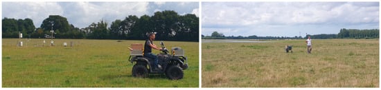
Figure 1.
Left: a view of the Toulo-Naizin agricultural measurement station and the motor quad used for SM measurements, equipped with a Cosmic Ray Neutron Sensor (CRNS). Right: View of the Marais de Sougéal natural wet meadows site and collection of SM data with the CRNS on top of a wheelbarrow.
2.2. UAV Flights and Image Processing
The CRNS Research Unit LETG team performed all drone flights using their available UAS, cameras and sensors between 09:00 and 12:00 UTC. Accordingly, three different sensors were flown over in separate flights on board fixed-wing and/or rotary-wing UAVs:
- MicaSense © RedEdge MX with 5 bands in the VNIR region: Blue (475 nm), Green (560 nm), Red (668 nm), RedEdge (717 nm) and near-infrared (842 nm) onboard of AgEagle eBee X—Flight height: 120 m a.g.l. Ground Sampling Distance = 8.4 cm. Image overlap: Lateral 70%, Frontal 75%. Flight duration 43–47 min. Radiance and irradiance captured on MicaSense © calibration panel before take-off.
- Thermal AgEagle Duet-T onboard of AgEagle eBee X (2 consecutive flights with 50 min time difference)—Flight height: 120 m a.g.l. Ground Sampling Distance = 14 cm. Image overlap: Lateral 70%, Frontal 75%. Flight duration 50–52 min.
- DJI Zenmuse L1 LiDaR onboard of DJI M350—Flight height: 70 m a.g.l. Average Point Cloud Density = 3413/m2. Flight speed 5 m/s; side overlap 50%; echo mode set to triple; LiDaR sample rate = 160 kHz; scan mode set to repeat. Generated Digital Elevation Model (DEM pixel size = 16.8 cm). Flight duration 39–45 min.
Although multispectral VNIR, thermal and LiDAR data can be used separately for SM mapping, other spectrum regions are much more sensitive to soil water content. However, our integrative approach seeks to benefit from combined multilayer data cubes, enabling statistical analysis to include indirect variables that are potentially related to SM variability.
A total of 20 ground control points (GCPs) were distributed homogeneously across the study sites to enhance and test geometric accuracy. Spatial information from all cameras and sensors was captured at both study sites and geometrically corrected using Agisoft Metashape software v. 2.2.1. and 50% of the available GCPs. The final orthomosaics, projected to EPSG:2154, were then combined in a multilayer spectral data cube (MSDC). The final spatial resolution of the MSDC was derived from the MicaSense RedEdge MX multispectral layer (8.4 cm) by resampling the other raster layers (thermal and DEM). All layers were co-registered using 50% of the available GCPs, and the final spatial accuracy was assessed using the remaining 50%. Although this resampling strategy implies redundant information for coarser layers, the unified MSDC spatial resolution relied on multispectral bands and derived indices as the most informative data for SM estimation.
All flights were carried out under homogeneous cloudy conditions with scattered incident sunlight on 25 and 26 July 2023 (agricultural and natural sites, respectively). Maximum drought was recorded for both sites during this summer period. Two reflectance panels were placed at the sites, and spectroradiometric measurements were taken using an ASD FieldSpec®, Analytical Spectral Devices, Boulder, CO, USA Full Range (400–2500 nm) spectroradiometer for vicarious calibration purposes [7]. An empirical line approach based on in situ spectroradiometric measurements from calibration panels located in the multispectral orthomosaics was applied to MicaSense multispectral reflectance images. Thermal images were acquired once the thermal sensor of AgEagle Duet-T had achieved temperature stabilisation. Brightness temperature was calculated using Pix4DMapper© v. 4.8.4. software and Land Surface Temperatures (LST) were derived using camera calibration values. No independent LST validation was carried out in the field.
2.3. In Situ SM Measurements
In situ soil volumetric water content (VWC) point measurements at a depth of 5 cm were carried out using a Theta Probe, which uses time domain reflectometry (TDR), along linear transects (six transects, 10 m between points, 122 TDR points) in the Sougéal wet meadows (see Figure 2), and at regular intervals around the permanent station in the agricultural area (25 m between points, 14 TDR points). At both sites, extensive sampling was performed using a portable Cosmic-Ray Neutron Sensor (CRNS) mounted on a motorised quad bike or wheelbarrow (see Figure 1), to cover the entire site area and maximise SM spatial variability. Mobile CRNS technology has been proven to provide volume-integrated soil moisture estimates over a horizontal footprint of hundreds of metres [8]. Unfortunately, the CRNS rover did not collect any neutron flux due to a malfunction. This led us to increase the sampling density of the TDR point for the natural site, as the malfunction was only confirmed after sampling on the agricultural site.
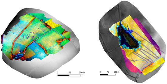
Figure 2.
Left: false colour (red: NIR, RedEdge) multispectral orthomosaic of the agricultural site on top of the produced digital elevation model (DEM) from a Zenmuse L1 camera, showing soil water content (SWC) point sampling locations (purple dots). Right: False colour (R: NIR, RedEdge) multispectral orthomosaic overlaid on thermal and DEM showing SWC point sampling locations (purple dots).
In situ measurements, GCPs and calibration panels were precisely geolocated using differential GNSS. We also collected spectral signatures for 10% of the sampling points using the portable ASD FieldSpec spectroradiometer.
2.4. Statistical Analysis and SM Mapping
To explore the most effective predictors, we used Generalised Linear Regression Models (GLRM) to estimate the VWC measured in situ. All spectral bands were used as predictors, as well as topographical height and the different spectral indices used in the literature for SM estimation [9], such as Normalized Difference Vegetation Index (NDVI), Normalized Difference RedEdge (NDRE), Normalized Difference Water Index (NDWI), Transformed Normalized difference vegetation index (TNDVI), Simple Ratio (SR), Soil Adjusted Vegetation Index (SAVI) and Perpendicular drought index (PDI). Most authors found an accurate relationship between soil moisture content (SMC) and surface reflectance (SR) using machine learning methods and a Micasense RedEdge-M camera. Additionally, we included ancillary predictors such as LST, which was retrieved using a ThermoMap camera, and the difference between two consecutive thermal flights (D_LST), in order to incorporate thermal inertia, which can be related to SMC [10]. For each sampling location, predictor values were extracted from the multilayer spectral data cube.
GLRM (Generalised Linear Model) enables the flexible generalisation of ordinary linear regression by relating the linear model to the response variable via a link function, while also allowing the magnitude of the variance of each measurement to be a function of its predicted value. Model fitting uses maximum likelihood in an iteratively reweighted least squares algorithm until the model is stable. Adjusted R2 provides a measure of goodness of fit, and root mean square error (RMSE) provides a measure of SM value uncertainty by comparing modelled and observed values. The best-fitted models were transferred for SM mapping purposes, applying only the predictors selected by the model over the full multispectral orthomosaic area.
3. Results
3.1. UAV Images
All UAV flights covered all in situ sampling points at both study sites (see Figure 2). The multispectral, thermal, and derived raster DEM from LiDAR data were co-registered using ground control points (GCPs) and unified in the MSDC with the same spatial resolution. The independent root mean square error (RMSE) calculated from the multispectral base layer was 4.76 cm and 3.14 cm.
Vicarious calibration by empirical line was only applied to the multispectral images, enabling comparisons to be made between the different flights and study sites, while accounting for the varying illumination conditions during each flight. The LST orthomosaic was not assessed on site, but the thermal gradient was considered to be representative of both study sites.
A visual assessment of multispectral orthomosaics reveals green vegetation patches, consisting of either trees or grasses, in contrast to areas of exposed bare soil covered by senescent herbs. In the natural wet meadow, the flooded areas show low NIR and RedEdge reflectance values, making them highly contrasting. The DEM derived from LiDAR data also provides good topographical detail, accurately representing the subtle topographical gradient, which is more evident in the natural study site. Thermal LST orthomosaics reveal spatial patterns that appear to be linked to topography and the water surface. D_LST captures temporal variation in LST, which is higher in the natural area. This reveals several D_LST hotspots in the flooded area and in the north-east, with temporal differences of up to 3.7 °C. In the agricultural area, maximum D_LST values were below 0.9 °C.
3.2. SM Modelling
The in situ VWC measurements ranged from 17 to 96% in the Sougéal wet meadows, while in the agricultural area they varied from 21.4 to 36.7%. This difference in range may increase uncertainty for the agricultural plot, where the number of in situ SM point measurements was also lower. Due to the failure of the CRNS rover, we could not use its extensive sampling to validate the final SM maps as originally planned, in order to achieve robust cross-validation across the two sites. Therefore, the uncertainty estimates rely on the adjusted R2 values of the fitted models, which used all the sampling points from both study sites.
The GLRM fitted to the wet meadows identified topographic height, extracted from the DEM, as the best predictor, followed by land surface temperature from the second thermal flight (11:50 h) and red band reflectance from the multispectral orthomosaic (see Figure 3). Statistical predictors selection was based on an associated probability of >0.05. The adjusted model for the wet meadows explained up to 62% of SM variability, with an RMSE of 12%. For the agricultural study site, however, the best predictor was only TNDVI, explaining 92% of the variance with an RMSE of 4.5%.
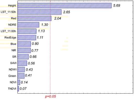
Figure 3.
Rank of the predictors for the SWC GLRM model for the Sougéal wet meadows according to t-values of coefficients (predictor variables). Red dashed line stands for significant values (p < 0.05).
3.3. Predictive SM Mapping
We used the models with the highest adjusted R2 values to predict spatially explicit SM gradients (Figure 4) for both agricultural and natural plots. Only selected predictors were considered.
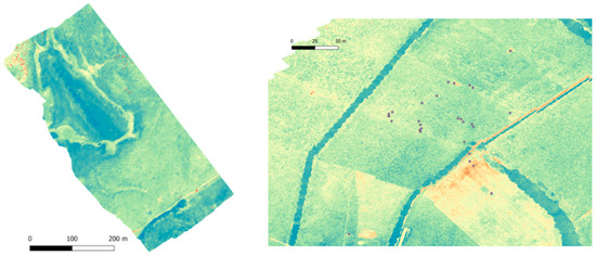
Figure 4.
Left: Predicted SM map of the Marais de Sougéal natural wet meadows. Right: Predicted SM map produced for the agricultural study site of Toulo-Naizin.
The predicted SM spatial maps adequately captured the observed in situ SM range, except for trees, which are modelled as having very high SM values. This bias is probably caused by leaf water content, which may be introduced by the red band reflectance in the wet meadow or the NIR/red band ratio used in the TNDVI calculation in the case of the agricultural site.
At the wet meadows site, topography clearly plays the most important role as the most explanatory predictor. The model also included LST from the second flight, revealing the effect of soil moisture on thermal emissivity [10]. However, the model did not select LST from either of the first two flights, nor from the difference between them.
In the case of the agricultural site, the modelled SM values are much lower and more uniform around the permanent measurement station than in the wet meadows. This spatial homogeneity of SM values confirms the representativeness of the location of the permanent SM probe for the entire plot. The neighbouring arable fields to the south are certainly drier, which reveals the sensitivity of the model.
In both study sites, some of the predicted SM variability can be attributed to vegetation cover and its water content.
4. Conclusions and Further Research
Although some of the multispectral and thermal bands were selected by the statistical models, the predicted SM maps seem to indirectly incorporate leaf water content, as evidenced by the trees’ high SM values. This kind of bias could be mitigated by incorporating SWIR bands or utilising radar systems equipped with ground-penetrating bands. A SWIR camera would improve the retrieval of leaf and soil water content, while radar would specifically detect surface SM due to its sensitivity to the presence of water, particularly in the L-band (1–2 GHz). However, few vendors are investing in such implementations, and only a few prototypes can be found on the market at very high cost.
Nevertheless, our results highlight the need to incorporate high-resolution SM mapping using drones in order to account for its inherent spatial variability, which is greater in natural areas. Crops dependent on rainfall, such as those we studied, are likely to be exposed to more frequent extreme droughts in the near future, which will compromise water availability more uniformly. Permanent stations will certainly be able to monitor declining trends representative of larger areas.
The agricultural study site produced more accurate results, likely due to a lower range of SM values. The natural site (wet meadows) showed higher SM variability, which probably contributed to lower SM mapping accuracy, although topographical height was an accurate, albeit indirect, predictor. Failure of CRNS technology resulted in lower in situ sampling density, which was more critical in the agricultural area and prevented us from implementing a more robust cross-validation.
SM maps such as those produced in this study could help to scale up and up-sample SM variability in satellite images, enabling the validation of products and improving accuracy irrespective of land cover.
Our study demonstrates the feasibility of applying similar methods to different habitats in order to quickly assess SM spatial variability. Repeated missions with the same sensors can contribute to tracking phenological and temporal changes, supporting seasonal drought assessment and response, and monitoring water stress.
Finally, while we took an empirical approach, applying GLRM to identify the most relevant SM predictors, future research should consider other methodological analyses, such as machine learning, deep learning, and physically based deterministic models.
Author Contributions
Conceptualization, R.D.-D. and O.F.; methodology, O.F., T.H. and R.D.-D.; field campaign, O.F., R.D.-D., P.B., T.P., Y.H., T.H. and M.F.; drone flights, T.H. and T.P.; data processing, T.H. and T.P.; statistical analyses, R.D.-D.; writing, review, and editing, R.D.-D.; graphical deployment, R.D.-D.; supervision, R.D.-D. All authors have read and agreed to the published version of the manuscript.
Funding
This study was funded by the eLTER Plus project (INFRAIA, Horizon 2020, Agreement no. 871128) through the granted Transnational Access project entitled “Upscaling of WAter Stress in AgroHydroSystems (UWASA)”. Partial funding was also provided by MICINN through European Regional Development Fund [SUMHAL, LIFEWATCH-2019-09-CSIC-4, POPE 2014-2020] and the research projects SpaFLEXVal (PID2022-137022OB-C33) and FLEX-S3 (PCI2023-145988-2) funded by MICIU/AEI/10.13039/501100011033/.
Acknowledgments
R.D.-D. is also a participant of the CSIC Interdisciplinary Thematic Platforms (PTI) PTI EcoBioDiv and PTI Teledetect and in the thematic network NetOps (RED2022-134438-T) funded by MICIU.
Conflicts of Interest
The authors declare no conflicts of interest. The funders had no role in the design of the study; in the collection, analyses, or interpretation of data; in the writing of the manuscript, or in the decision to publish the results.
Abbreviations
The following abbreviations are used in this manuscript:
| SM | Soil Moisture |
| CRNS | Cosmic-Ray Neutron Sensor |
| TNDVI | Transformed Normalized Difference Vegetation Index |
| UAV | Unmanned Aerial Vehicle |
References
- Vogel, M.M.; Zscheischler, J.; Seneviratne, S.I. Varying Soil Moisture–Atmosphere Feedbacks Explain Divergent Temperature Extremes and Precipitation Projections in Central Europe. Earth Syst. Dyn. 2018, 9, 1107–1125. [Google Scholar] [CrossRef]
- Babaeian, E.; Sadeghi, M.; Jones, S.B.; Montzka, C.; Vereecken, H.; Tuller, M. Ground, Proximal, and Satellite Remote Sensing of Soil Moisture. Rev. Geophys. 2019, 57, 530–616. [Google Scholar] [CrossRef]
- Ohnemus, T.; Zacharias, S.; Dirnböck, T.; Bäck, J.; Brack, W.; Forsius, M.; Mallast, U.; Nikolaidis, N.P.; Peterseil, J.; Piscart, C.; et al. The eLTER Research Infrastructure: Current Design and Coverage of Environmental and Socio-Ecological Gradients. Environ. Sustain. Indic. 2024, 23, 100456. [Google Scholar] [CrossRef]
- Sun, H.; Liu, H.; Ma, Y.; Xia, Q. Optical Remote Sensing Indexes of Soil Moisture: Evaluation and Improvement Based on Aircraft Experiment Observations. Remote Sens. 2021, 13, 4638. [Google Scholar] [CrossRef]
- Kim, S.; Zhang, R.; Pham, H.; Sharma, A. A Review of Satellite-Derived Soil Moisture and its Usage for Flood Estimation. Remote Sens. Earth Syst. Sci. 2019, 2, 225–246. [Google Scholar] [CrossRef]
- Dubreuil, V.; Dubreuil, V.; Lamy, C.; Planchon, O. Les sécheresses à Rennes: Passé, présent et futur. In Actes du Colloque: Les Risques Naturels dans le Contexte du Changement Climatique; Holobâcâ, I.-H., Ivan, K., Eds.; Rennes, France, 2018; pp. 15–21. Available online: https://shs.hal.science/halshs-01825987v2 (accessed on 24 August 2025).
- Bannari, A.; El-Ghmari, A.; Rhinane, H.; Selouani, A.; Loulad, S. Vicarious Radiometric Calibration of UAV-Data in Mountainous Area Using Semi-Empirical Line Approach and In-Situ Spectroradiometric Measurements. In Proceedings of the IGARSS 2024–2024 IEEE International Geoscience and Remote Sensing Symposium, Athens, Greece, 7–12 July 2024; pp. 6384–6387. [Google Scholar]
- Fersch, B.; Francke, T.; Heistermann, M.; Schrön, M.; Döpper, V.; Jakobi, J.; Baroni, G.; Blume, T.; Bogena, H.; Budach, C.; et al. A Dense Network of Cosmic-Ray Neutron Sensors for Soil Moisture Observation in a Highly Instrumented Pre-Alpine Headwater Catchment in Germany. Earth Syst. Sci. Data 2020, 12, 2289–2309. [Google Scholar] [CrossRef]
- Khose, S.B.; Mailapalli, D.R. Spatial Mapping of Soil Moisture Content Using Very-High Resolution UAV-Based Multispectral Image Analytics. Smart Agric. Technol. 2024, 8, 100467. [Google Scholar] [CrossRef]
- Wienhold, K.J.; Li, D.; Fang, Z.N. Precision Irrigation Soil Moisture Mapper: A Thermal Inertia Approach to Estimating Volumetric Soil Water Content Using Unmanned Aerial Vehicles and Multispectral Imagery. Remote Sens. 2024, 16, 1660. [Google Scholar] [CrossRef]
Disclaimer/Publisher’s Note: The statements, opinions and data contained in all publications are solely those of the individual author(s) and contributor(s) and not of MDPI and/or the editor(s). MDPI and/or the editor(s) disclaim responsibility for any injury to people or property resulting from any ideas, methods, instructions or products referred to in the content. |
© 2025 by the authors. Licensee MDPI, Basel, Switzerland. This article is an open access article distributed under the terms and conditions of the Creative Commons Attribution (CC BY) license (https://creativecommons.org/licenses/by/4.0/).