Linear Quadratic Regulator Control of Rotary Inverted Pendulum Using Elvis III Embedded Platform ^†

Abstract

Modern education is characterized by diversity and the need for extensibility. Educational experimental platforms are rapidly evolving according to these factors. However, software and hardware are provided by major domestic manufacturers, which imposes limitations on the development of teaching materials. We investigate the implementation of a rotational inverted pendulum control system within the NI ELVIS III embedded system. The mathematical model of the rotational inverted pendulum is constructed using Lagrangian equations and then represented in matrix form. Following linearization of the nonlinear state equations, the linear quadratic regulator (LQR) controller of the rotational inverted pendulum apparatus is designed and implemented on the NI ELVIS III embedded system by using LabVIEW graphical programming software. Illustrations are generated to compare the continuous tracking performance of LQR and PID controllers with preset target values. The results are then analyzed to evaluate and contrast the effectiveness of both control strategies in tracking the target values. The findings of this study enhance the development of educational content related to the ELVIS III embedded system’s experimental platform.

1. Introduction

The inverted pendulum system is an extended application of the motor control system. It has nonlinear system characteristics and a simple structure so it is often used as a research object of control systems to verify the practicability of various control theories. National Instruments Corporation (NI) is an instrument and equipment manufacturer researching and developing automated testing and measurement systems and providing related solutions. NI Engineering Laboratory Instrumentation Suit III (ELVIS III) [1] is a programable Xillinx 7020 FPGA embedded teaching platform. The ELVIS III platform consists of an analog input, analog output, digital input, digital output, power supply, oscilloscope, signal generator, and breadboard interface. It enables Bode analysis, oscilloscope analysis, function generation, impedance analysis, Logic analysis, controllable power supplying, and digital electricity meter function. In addition, it provides a driver interface for LabView, Matlab, and other programming environments.

With the help of a graphical programming interface, researchers can design and analyze controller development to propose a quick design solution with a controller for the controlled system to make the control program’s verification easy and shorten product development time. Reference [2] researched the continuous- and discrete-time states of the Riccati Equation to solve optimization problems. Agarana et al. discussed the dynamics of the inverted pendulum derived by the Lagrangian model [3], and they used the Laplace transform algorithm to easily generate and solve algebraic equations.

The dynamic system of the inverted pendulum is consistent with the second-order differential equation model of the dynamic system. The Furuta pendulum system was studied in Ref. [4]. Several linearized points are unobservable in this system, so an iterative learning control was proposed to improve transient trajectory response based on a matrix with a uniform distribution of observable points. Simulation results demonstrate that this method is feasible for this system. A nonlinear controller with friction compensation is presented in Ref. [5]. An energy controller was used to solve the three problems caused by friction that occurred when the inverted pendulum swung: the swing rod could not achieve a complete swing, did not fully reach the equilibrium position, and took a long time to swing up and stabilize. The control and design of the inverted pendulum were studied in Refs. [6,7,8].

A discrete-action space reinforcement learning method (Q-learning) was proposed for the robot to learn continuous-time control of inverted pendulum balance [9]. This research demonstrated the feasibility of a simulated environment for a control system placed on a real robot. Based on the result, continuous-action control using discrete-action space algorithms can be used, and through a simulation, training time and the risk of hardware damage decreases.

In this study, we integrate the rotary inverted pendulum system and LabView as the controller design environment into the ELVIS III embedded control system. A simple linear controller developed from the LQR algorithm is uploaded to the embedded system, the ELVIS III experimental platform, to test the controller’s performance within the rotating inverted pendulum nonlinear system.

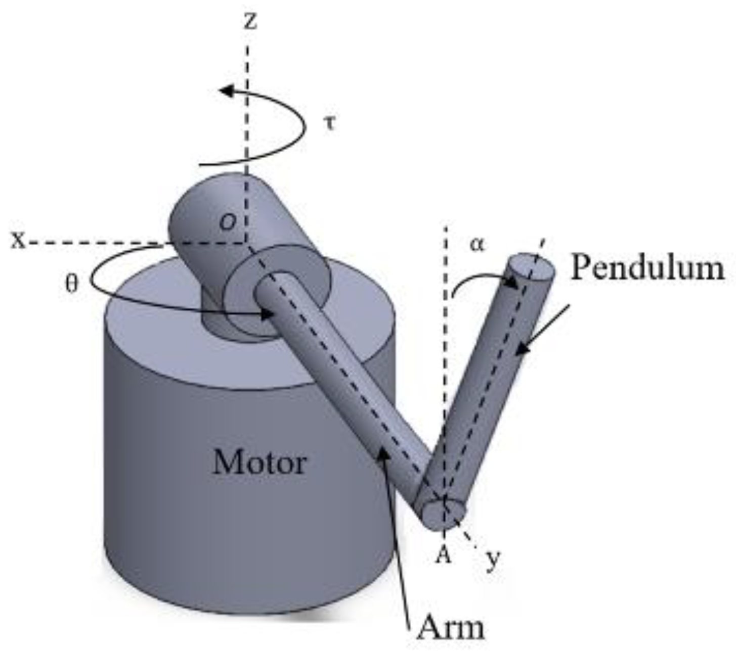
2. Dynamic Model of Rotary Inverted Pendulum

The rotary inverted pendulum (Figure 1) is merged with the DC motor [10,11]. Its dynamic equation can be expressed by (1), and its parameters are defined in

Table 1. System parameters.

Symbol	Description	Value	Unit
Lp	Swing bar length	0.08504	m
mp	Swing bar mass	0.01724	Kg
Lr	Swing arm length	0.10602	M
mr	Swing arm mass	0.06046	Kg
g	Gravity	9.81	m/s2
Jp	Equivalent inertia of the swing rod	0.00003143	kg·m2
Jr	Equivalent inertia of rotating arm	0.00067416	kg·m2
C1	The distance from the pivot point O to the center of mass G1 of the rotating arm	0.01606	M
C2	The distance from the pivot point A to the center of mass G2 of the swing rod	0.04321	M
Kb	Back electromotive force	0.16344417	V·s/rad
Kt	Motor torque constant	0.16344417	N·m/A
Ra	Armature resistance	6.15	Ω

.

$$M\ddot{x}+C_m\dot{x}+Gx=V\cdot e(t)$$

(1)

where:

$$M=\left[\begin{array}{cc}{P}_1+P_2{\sin }^2\alpha & P_3\cos \alpha \\ P_3\cos \alpha & P_2\end{array}\right]$$

$$C_m=\left[\begin{array}{cc}\frac{1}{2}{P}_2\dot{\alpha }\sin 2\alpha & \frac{1}{2}{P}_2\dot{\theta }\sin 2\alpha -P_3\dot{\alpha }\sin \alpha \\ -\frac{1}{2}{P}_4\dot{\theta }\sin 2\alpha & 0\end{array}\right]$$

$$G=\left[\begin{array}{c}0\\ -P_5\sin \alpha \end{array}\right], V=\left[\begin{array}{c}{P}_7\\ 0\end{array}\right]$$

$$P_1=J_r+m_p{L}_r^2, P_2=m_p{C}_2^2+J_p, P_3=m_p{L}_r{c}_2, P_4=m_p{c}_2^2,$$

$$P_5=m_{p}g{c}_2, P_6=K_t{K}_b/R_a, P_7=K_t/R_a.$$

Next, the system state variable is set as follows:

$$x_1=\theta , x_2=\alpha , x_3=\dot{\theta }, x_4=\dot{\alpha }$$

(2)

Therefore, the nonlinear state-space equations of the system are as follows:

$${\dot{x}}_1=x_3$$

(3)

$${\dot{x}}_2=x_4$$

(4)

$$\begin{gathered} {\dot{x}}_3=\frac{1}{\Delta }\{-\sin (2x_2)[P_2^2{x}_3{x}_4+P_3{P}_4{x}_3^2\cos (x_2)+\frac{1}{2}{P}_3{P}_5] \\ \hspace{1em}\hspace{1em}\hspace{1em}\hspace{1em}-P_2{P}_6{x}_3+P_2{P}_3{x}_4^2\sin (x_2)+P_2{P}_{3}e\} \end{gathered}$$

(5)

$$\begin{gathered} \begin{array}{l}{\dot{x}}_4=\frac{1}{\Delta }\{\sin (2x_2)[P_1{P}_4{x}_3^2+P_2{P}_4{x}_3^2{\sin }^2(x_2)+P_2{P}_3{x}_3{x}_4\cos (x_2)\\ \hspace{1em}\hspace{1em}-\frac{1}{2}{P}_3^2{x}_4^2]+\sin (x_2)[P_1{P}_5+P_2{P}_5{\sin }^2(x_2)]\end{array} \\ \hspace{1em}\hspace{1em}\hspace{1em}\hspace{1em}\hspace{1em}\hspace{1em}\hspace{1em}\hspace{1em}\hspace{1em}\hspace{1em}\hspace{1em}\hspace{1em}+\cos (x_2)[P_3{P}_6{x}_3-P_3{P}_{7}e]\} \end{gathered}$$

(6)

$$\Delta =P_1{P}_2+P_2^2{\sin }^2(x_2)-P_3^2{\cos }^2(x_2)$$

(7)

Then, the above equations can be expressed as follows:

$$\dot{X}=f(x,e)$$

(8)

X = [x₁, x₂, x₃, x₄]^T and let the unstable point at the upper position of the inverted pendulum be an equilibrium point, X_e = [0, 0, 0, 0]^T. Then, the system is linearized according to this point.

$$\delta \dot{X}={\left.{\displaystyle \frac{\partial f}{\partial x}}\right|}_{X_e}\cdot \delta X+{\left.{\displaystyle \frac{\partial f}{\partial e}}\right|}_{X_e}\cdot e=A\cdot \delta X+B\cdot e$$

(9)

where:

$$A=\left[\begin{array}{cccc}0& 0& 1& 0\\ 0& 0& 0& 1\\ 0& -\frac{P_3{P}_5}{P_1{P}_2-P_3^2}& -\frac{P_2{P}_6}{P_1{P}_2-P_3^2}& 0\\ 0& \frac{P_1{P}_5}{P_1{P}_2-P_3^2}& \frac{P_3{P}_6}{P_1{P}_2-P_3^2}& 0\end{array}\right]$$

$$B=\left[\begin{array}{cccc}0& 0& \frac{P_2{P}_7}{P_1{P}_2-P_3^2}& -\frac{P_3{P}_7}{P_1{P}_2-P_3^2}\end{array}\right]$$

The output equation of the control system is as follows:

$$Y=CX=\left[\begin{array}{cccc}1& 0& 0& 0\\ 0& 1& 0& 0\end{array}\right]X$$

(10)

3. LQR Controller Design

The LQR is a state-space design method [12]. The LQR refers to the design of the optimal-state feedback controller to minimize the quadratic objective function, and the gain of the controller is determined by the weight matrices Q and R. Therefore, the selection of Q and R plays an essential role in obtaining the feedback gain value of the controller for stabilizing the system. We first consider the state equation of the linear non-time-varying dynamic system as follows:

$$\dot{x}=Ax+Bu$$

(11)

$$y=Cx$$

(12)

where x is the state vector, u is the control input, y is the system output, and A, B, and C are the constant matrices. According to the optimal control of the linear quadratic Gaussian method, the cost function J is selected as follows:

$$J={\displaystyle {\int }_0^{\infty }\left(x{(t)}^{T}Qx(t)+u^T(t)Ru(t)\right)}dt$$

(13)

where Q = Q^T ≥ 0 is a positive semi-definite matrix, and R^T > 0 is a positive definite matrix. To have the minimum cost function value under relative control u, the algebraic Riccati Equation (14) must be satisfied.

$$A^{T}P+PA+Q-K^T{B}^{T}P-PBK+K^{T}RK=0$$

(14)

The optimal feedback gain K_x of its steady-state solution is as follows:

$$K_x=R^{-1}{B}^{T}P$$

(15)

Finally, the Riccati Equation is simplified as follows:

$$A^{T}P+PA-PB{R}^{-1}{B}^{T}P+Q=0$$

(16)

Finally, the linear state feedback controller u = -K_x⋅x is the optimal controller for the LQR that can minimize the performance of the cost function.

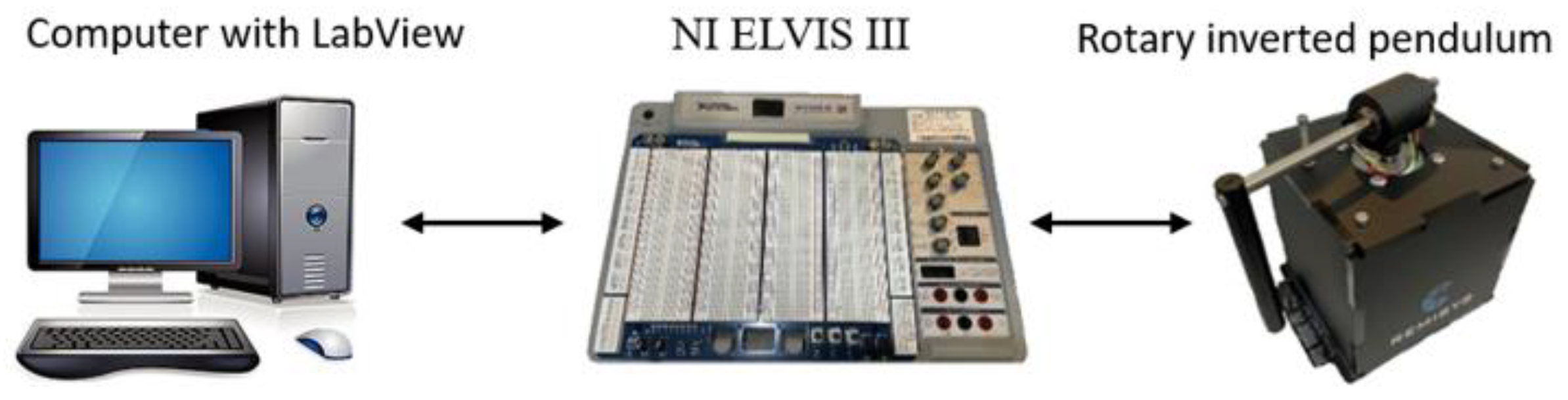
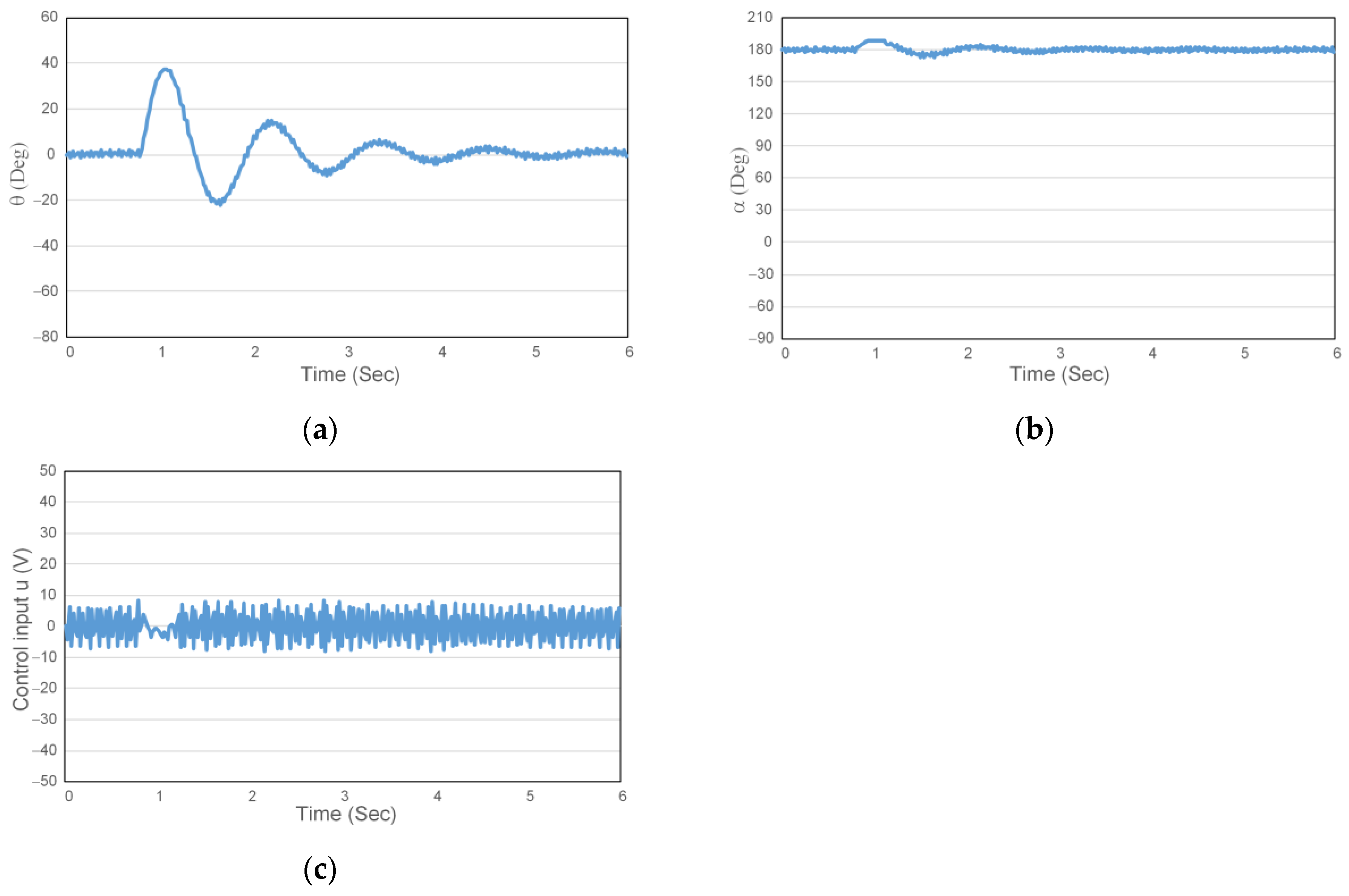
4. Experimental Results

The rotary inverted pendulum experimental system is shown in Figure 2, and its parameters are shown in Table 1. Through the linearization of the system’s dynamic model concerning the equilibrium point and substituting the system’s parameters, the following equations are obtained.

$$\left[\begin{array}{c}\dot{\theta }\\ \dot{\alpha }\\ \ddot{\theta }\\ \ddot{\alpha }\end{array}\right]=\left[\begin{array}{cccc}0& 0& 1& 0\\ 0& 0& 0& 1\\ 0& 92.53& 0.007& 0\\ 0& -0.153& -54.99& 0\end{array}\right]\left[\begin{array}{c}\theta \\ \alpha \\ \dot{\theta }\\ \dot{\alpha }\end{array}\right]+\left[\begin{array}{c}0\\ 0\\ -0.004\\ 336.5\end{array}\right]u(t)$$

(17)

According to the above formula, the optimization parameters Q and R of the LQR are designed as follows:

$$Q=\left[\begin{array}{cccc}25& 0& 0& 0\\ 0& 25& 0& 0\\ 0& 0& 1& 0\\ 0& 0& 0& 2.5\end{array}\right], R = 2.5$$

(18)

First, the feedback gain K_x = [3.16 15.65 1.05 1.04] is obtained after calculating the rotating inverted pendulum model and the Q and R weight matrices. Application of the controller is divided into two steps. The first step is the swing action. The second step is to switch to LQR closed-loop control when the pendulum is swung to a certain angle. Then, the LQR control experimental results of the rotating inverted pendulum can be obtained.

Figure 3 shows the angular displacement of the rotating arm (angle), the angular displacement of the swinging arm, the angular velocity of the rotating arm, the angular velocity of the swinging arm, and the control input of the rotating arm to time. The rotating arm θ moves left and right in the beginning from the start point to 17.5°, then in the opposite direction to −40°, and then moves significantly to a position of 41° (Figure 3a). This demonstrates the swing action that forces the swing rod to swing up. At this time, the swing rod α in Figure 3b moves as the rotating arm θ moves. A greater swing amplitude is obtained until it switches to equilibrium and then remains at a position 180° to the equilibrium point. Figure 3c and d, respectively, show the angular velocity of the rotating arm and the angular velocity of the swing rod. In this experiment, the angular velocity of the rotating arm reaches a maximum of 900 (angle/second) and stabilizes within 200 (angle/second). The angular velocity of the swing rod reaches a maximum of 1599 (angle/second) and then stabilizes within 250 (angle/second). The control input u reaches a maximum of −45 (V) when input to the rotating arm motor and oscillates within a 10 (V) range after stabilization, as shown in Figure 3e.

An external force interferes with the inverted pendulum when the system is steady. For example, by lightly touching the swing rod with a finger, stability changes are observed during the control period. Figure 4 shows the angular displacement of the rotating arm, the swinging arm, and the control input of the rotating arm. After stabilization, the inverted pendulum is moved with the touch of a finger. In this incident, the control input u is vastly changed, initially to quickly control the swing rod and bring it back to the equilibrium point (Figure 4). At this time, the θ angle of the rotating arm in Figure 4a is disturbed, and there is an apparent angular displacement. Upon reaching the maximum degree of 37.5, the shaking amplitude becomes smaller after correction over time until it returns to the stable equilibrium point. It takes about 5 s for the LQR controller to return the swing rod to the equilibrium point when the inverted pendulum starts to be interfered with.

5. Conclusions

The LQR-optimized state-space feedback controller has been successfully designed and applied for the control of a rotating inverted pendulum by integrating LabView and ELVIS III embedded systems. The controller is adjusted through the Q and R weight matrices to minimize the positioning error and has appropriate energy characteristics and anti-interference stability. Experiment results have verified that this method has the advantages of stable control performance and anti-interference when changing the positioning command. In addition, because the controller uses linear feedback, the overall control performance becomes better than that of the PID controller. Future research is necessary to design and control a rotating double-link inverted pendulum system or propose an advanced controller design to further improve control performance and anti-interference stability.

References

1. Available online: https://www.ni.com/zh-tw/shop/model/ni-elvis-iii.html (accessed on 12 October 2024).
2. György, K.; Dávid, L.; Kelemen, A. Theoretical study of the nonlinear control algorithms with continuous and discrete-time state-dependent Riccati equation. Procedia Technol. 2016, 22, 582–591. [Google Scholar] [CrossRef]
3. Agarana, M.C.; Akinlabi, E.T. Lagrangian-Laplace dynamic mechanical analysis and modeling of inverted pendulum. Procedia Manuf. 2019, 35, 711–718. [Google Scholar] [CrossRef]
4. Binz, R.; Aranovskiy, S. Iterative learning control strategy for a Furuta pendulum system with variable-order linearization. IFAC-PapersOnLine 2021, 54, 14–19. [Google Scholar] [CrossRef]
5. Antonio-Cruz, M.; Hernandez-Guzman, V.M.; Merlo-Zapata, C.A.; Marquez-Sanchez, C. Nonlinear control with friction compensation to swing-up a Furuta pendulum. ISA Trans. 2023, 139, 713–723. [Google Scholar] [CrossRef] [PubMed]
6. Nekoo, S.R. Digital implementation of a continuous-time nonlinear optimal controller: An experimental study with real-time computations. ISA Trans. 2020, 101, 346–357. [Google Scholar] [CrossRef] [PubMed]
7. Acuña-Bravo, W.; Molano-Jiménez, A.G.; Canuto, E. Embedded model control for underactuated systems: An application to Furuta pendulum. Control. Eng. Pract. 2021, 113, 104854. [Google Scholar] [CrossRef]
8. Nisar, L.; Koul, M.H.; Ahmad, B. Controller design aimed at achieving the desired states in a 2-DOF rotary inverted pendulum. IFAC-PapersOnLine 2024, 57, 256–261. [Google Scholar] [CrossRef]
9. Safeea, M.; Neto, P. A Q-learning approach to the continuous control problem of robot inverted pendulum balancing. Intell. Syst. Appl. 2024, 21, 200313. [Google Scholar] [CrossRef]
10. Tejado, I.; Torres, D.; Pérez, E.; Vinagre, B.M. Physical modeling based simulators to support teaching in automatic control: The rotatory pendulum. IFAC-PapersOnLine 2016, 49, 75–80. [Google Scholar] [CrossRef]
11. Yavin, Y. Control of a rotary inverted pendulum. Appl. Math. Lett. 1999, 12, 131–134. [Google Scholar] [CrossRef]
12. Franklin, G.F.; Powell, J.D.; Workman, M. Digital Control of Dynamic Systems, 3rd ed.; Ellis-Kagle Press: Half Moon Bay, CA, USA, 1998. [Google Scholar]
Figure 1. Schematic diagram of rotary inverted pendulum.
Engproc 92 00046 g001
Figure 2. Architecture of rotary inverted pendulum control system.
Engproc 92 00046 g002
Figure 3. The experimental results using the LQR controller: (a) The angular displacement of the rotating arm, (b) the angular displacement of the swinging arm, (c) the angular velocity of the rotating arm, (d) the angular velocity of the swinging arm, and (e) the control input of the rotating arm.
Engproc 92 00046 g003
Figure 4. Control results of rotary inverted pendulum with external disturbance: (a) angular displacement of rotating arm, (b) angular displacement of swinging arm, and (c) control input of rotating arm.
Engproc 92 00046 g004