
Real-Time Head Orientation and Eye-Tracking Algorithm Using Adaptive Feature Extraction and Refinement Mechanisms †


Abstract
1. Introduction
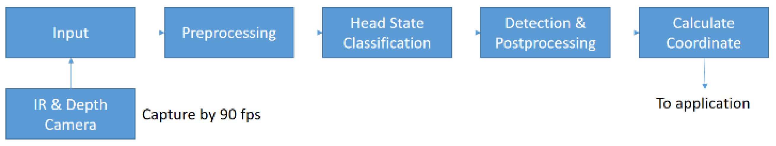
2. Method
2.1. Input Images
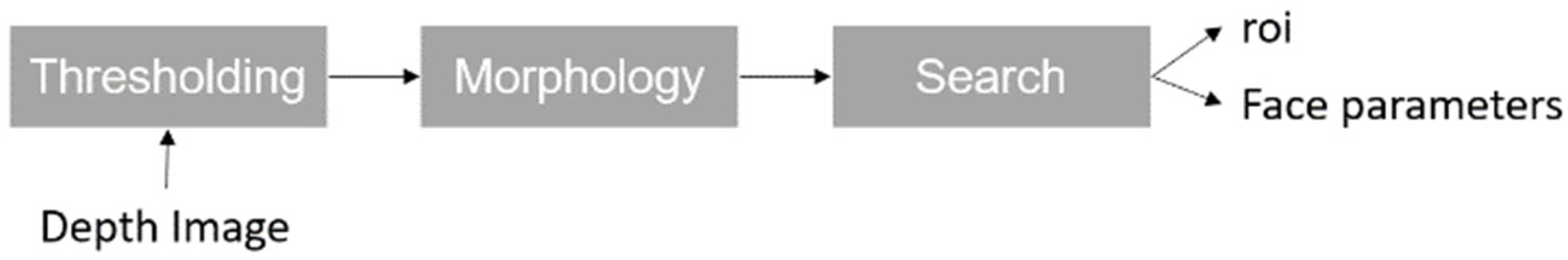
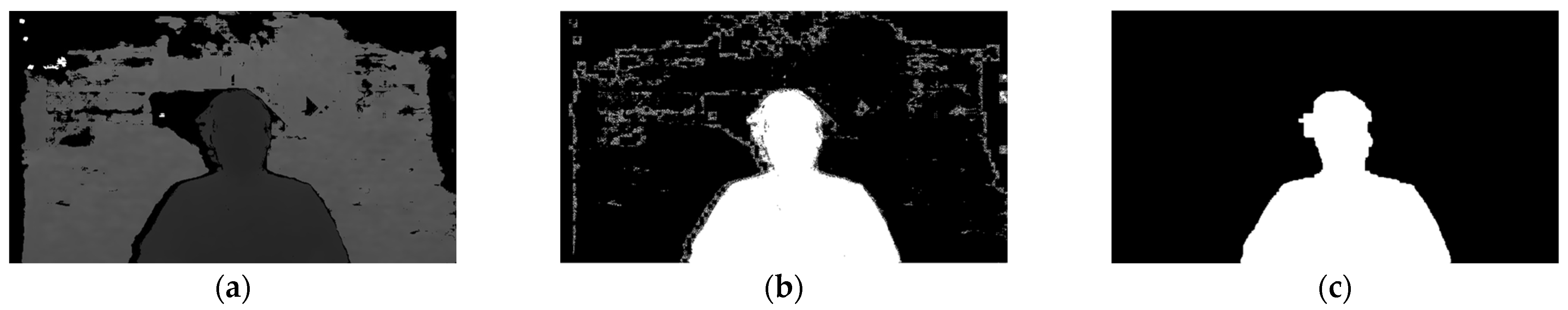
2.2. Preprocessing
2.3. Head State Classification
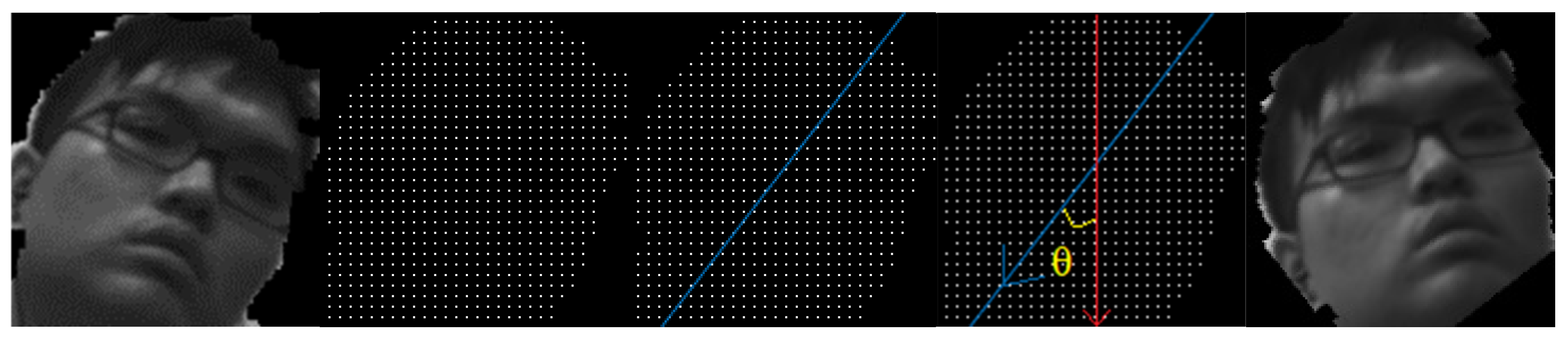
2.3.1. Roll
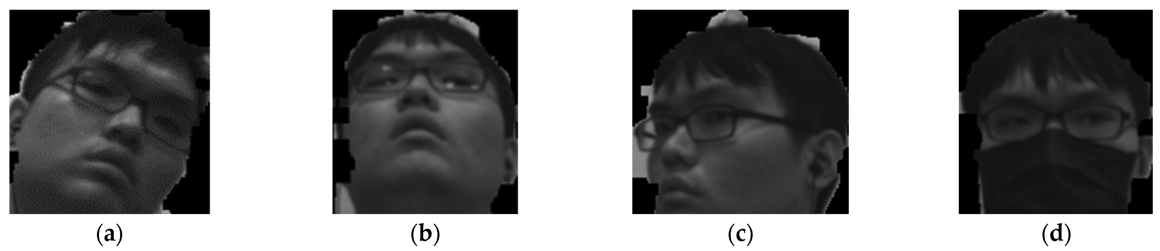
2.3.2. Pitch-Up, Yaw, and Mask
2.3.3. Pitch Down
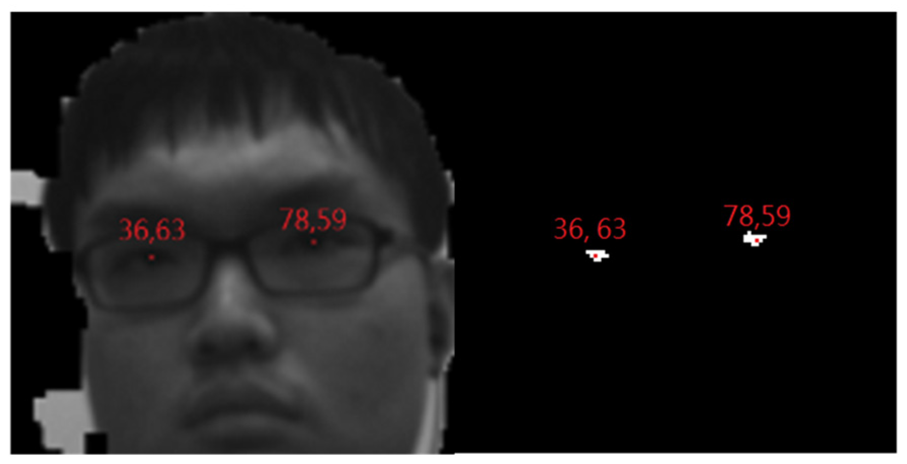
2.4. Detection and Postprocessing
2.5. Coordinate Transformation and Correction
3. Discussions
3.1. Detection Rates in Different Cases
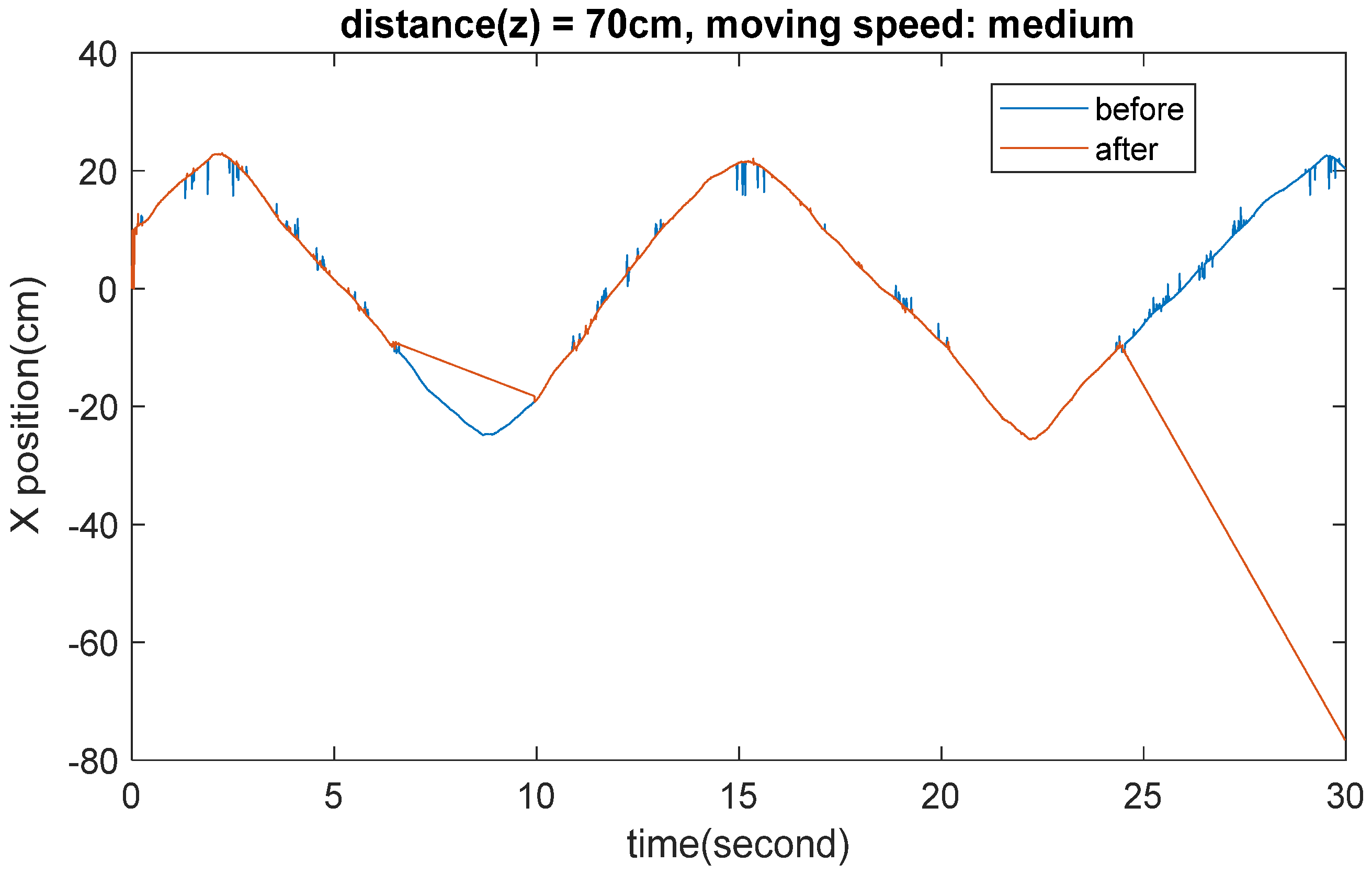
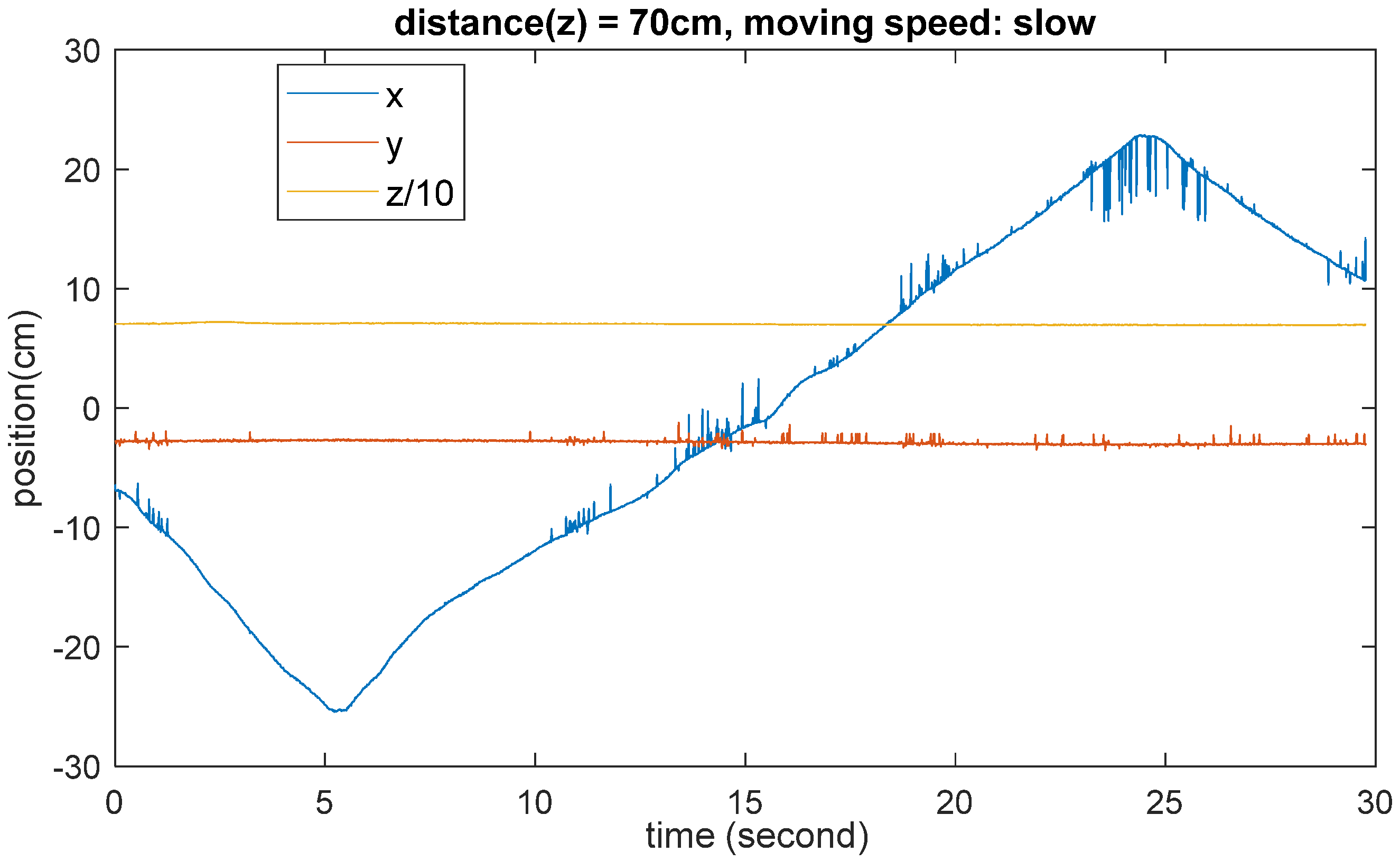
3.2. Accuracy and Stability
4. Conclusions
Author Contributions
Funding
Institutional Review Board Statement
Informed Consent Statement
Data Availability Statement
Acknowledgments
Conflicts of Interest
References
- Satoh, K.; Kitahara, I.; Ohta, Y. 3D Image Display with Motion Parallax by Camera Matrix Stereo. In Proceedings of the Third IEEE International Conference on Multimedia Computing and Systems, Hiroshima, Japan, 17–23 June 1996; pp. 349–357. [Google Scholar]
- Wijewickrema, S.N.R.; Papliński, A.P. Principal Component Analysis for The Approximation of an Image as an Ellipse. In Proceedings of the 13th International Conference in Central Europe on Computer Graphics, Visualization and Computer Vision 2005, Plzen, Czech Republic, 31 January–4 February 2005; pp. 69–70. [Google Scholar]
- Vincent, O.R.; Folorunso, O. A Descriptive Algorithm for Sobel Image Edge Detection. Informing Sci. IT Educ. Conf. 2009, 40, 97–107. [Google Scholar]
- Jiang, B.N. On The Least-Squares Method. Comput. Methods Appl. Mech. Eng. 1998, 152, 239–257. [Google Scholar] [CrossRef]


| Step 1 | |
| Step 2 | , we call the 1-pixel “valid” |
| Step 3 | When both r and c are multiple of 5, push it into a set of pixel coordinates, P |
| Step 4 | Stop condition: the number of the rows which have been searched exceed |
| Step 5 | “roi” is the smallest rectangle that contains all “valid” 1-pixels |
| Step 6 | Average depth and intensity are also recorded |
| Step 7 | Performing PCA on P to find tilting angle θ. [2] |
| Step 8 | Resize the image by |
| States | Meaning | Possible Values | Meanings |
|---|---|---|---|
| Pitch | The head lifted or fallen. | ‘\0’, ‘U’, ‘D’ | None, Up, Down |
| Roll | The head tilted left or right. | ‘\0’, ‘L’, ‘R’ | None, Left, Right |
| Yaw | The head turns left or right | ‘\0’, ‘L’, ‘R’ | None, Left, Right |
| Mask | Whether wears a mask. | False, True | No, Yes |
| (Mask, Pitch, Yaw) | IR Image | Edge Distribution |
|---|---|---|
| (0, ‘\0’, ‘\0’) |  | 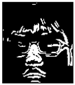 |
| (0, ‘\0’, ‘L’ or ‘R’) |  |  |
| (0, ‘U’, ‘\0’) |  | 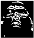 |
| (1, ‘\0’, ‘\0’) |  |  |
| (1, ‘\0’, ‘L’ or ‘R’) |  | 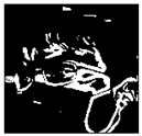 |
| (1, ‘U’, ‘\0’) |  | 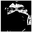 |
| Step 1 | Erode (F != 0) by a 1 rows by 23 columns kernel, we obtain a binary image F′. |
| Step 2 | |
| Step 3 | is the midpoint of 1-pixels at i-th row of F’ and M is the number of rows of F |
| Step 4 | In this step, we search for the three regions: (a) (b) (c) in each region, denote them as respectively. |
| Step 5 | (1) If && ( and < 0.15 || abs( − ) < 0.1): Mask ‘\0’, procedure stops (2) If ( or 0.15 && abs( − ) 0.1: Mask ‘\0’. Yaw ‘L’, procedure stops ‘R’, procedure stops. |
| Step 6 | Search for and where N is the number of columns of and . The former is the standard deviation of the row coordinates of all found 1-pixels, and the latter is the average value of column coordinates of all found 1-pixels. In addition, calculate and , the number of 1-pixels located at the upper half and bottom half of the search region, then calculate . |
| Step 7 | for the same range as that in step 7. 0.01: Mask ← True, Pitch ← ‘U’, Yaw ← ‘\0’, procedure stops. Also, calculate , which is the standard deviation of the column (x) coordinates of all found 1-pixels in the searching of in this step. |
| Step 8 | (1) If > 0.125N && ( < 0.1M || > 0.8): Mask ‘\0’, procedure stops. (2) If > 0.125N && 0.1M: Mask ‘\0’. closer to L: Yaw ‘L’, procedure stops. (3) If 0.125N: Mask ‘\0’, procedure stops |
| Step 1 | Search and all c. |
| Step 2 | ‘D’ |
| Step 1 | along Mids[i]. i start at 0.1M, But if Yaw != ‘\0’ or Pitch == ‘D’, start at 0.2M. | |
| Step 2 | (i, Mids[i]) != 0, procedure stops and record i. | |
| Step 3 | Pitch == ‘U’ | up i + 0.05M, if up > 0.3M, set it to be 0.3M. |
| Pitch == ‘D’ | up i + 0.1M, if up > 0.7M or <0.5M, set it to be 0.7M or 0.5M. | |
| Yaw != ‘\0’ | up i + 0.1M, if up > 0.4M or <0.3M, set it to be 0.4M or 0.3M. | |
| No pitch & yaw | up i + 0.1M, if up > 0.4M or <0.25M, set it to be 0.4M or 0.25M. | |
| Step 4 | Pitch == ‘U’ | low up + 0.25M |
| Not pitch up | low up + 0.3M | |
| Step 5 | left ← Mids[ Mids[] + 0.35N | |
| Mask off | No Yaw&Pitch | |
| Pitch up | ||
| Pitch down or Yaw | ||
| Mask on | No Pitch&Yaw | |
| Pitch up | ||
| Pitch down | ||
| Yaw |
| State | Distance | Y-Position | Other |
|---|---|---|---|
| Yaw != ‘\0’ | 0.15N~0.4N | Overlapped by range 2 | Width both < 0.1N |
| Pitch == ‘U’ | 0.3N~0.5N | Overlapped by range 0 | |
| else | 0.3N~0.5N |
| Mask | Orientation | Successful Frame/All Frame | Detection Rate |
|---|---|---|---|
| off | Normal | 957/988 | 0.968623 |
| Yaw | 820/902 | 0.909091 | |
| Pitch up | 843/938 | 0.898721 | |
| Pitch down | 476/581 | 0.819277 | |
| on | Normal | 898/999 | 0.898899 |
| Yaw | 772/911 | 0.84742 | |
| Pitch up | 777/901 | 0.862375 | |
| Pitch down | 326/407 | 0.800983 |
| Degree | acc_x (mm) | acc_y (mm) | acc_z (mm) | pre_x (mm) | pre_y (mm) | pre_z (mm) | shift_x (mm) | shift_y (mm) | shift_z (mm) |
|---|---|---|---|---|---|---|---|---|---|
| −18.88 | −2.4492 | −3.4629 | 0.8525 | 0.6194 | 0.6164 | 0.555 | 2.5382 | 3.7481 | 1.6015 |
| −14.51 | −2.6547 | −4.1006 | −0.1107 | 0.5741 | 0.5359 | 0.6304 | 2.4783 | 3.0624 | 2.5647 |
| −9.85 | −1.8524 | −4.0964 | 0.1772 | 0.6375 | 0.5396 | 0.6323 | 3.0258 | 3.2125 | 2.2768 |
| −4.98 | −0.431 | −4.3965 | −0.1065 | 0.7668 | 0.7185 | 0.6496 | 3.037 | 8.8755 | 2.5605 |
| 0 | 0.1263 | −4.5644 | −0.2726 | 0.6634 | 0.6055 | 0.5406 | 4.6565 | 2.8621 | 1.7316 |
| 4.98 | 0.4748 | −5.0363 | −0.17 | 0.6156 | 0.5305 | 0.5882 | 2.6783 | 2.4536 | 2.624 |
| 9.85 | 1.512 | −5.292 | −0.6269 | 0.6749 | 0.5539 | 0.6578 | 2.9627 | 3.0016 | 3.0809 |
| 14.51 | 2.4336 | −5.2404 | −2.8617 | 0.7007 | 0.6676 | 0.7664 | 2.9136 | 3.1101 | 2.3307 |
| 18.88 | 3.2321 | −5.7841 | −0.4962 | 0.6968 | 0.5597 | 0.6014 | 3.8441 | 3.5357 | 3.0198 |
| Degree | acc_x (mm) | acc_y (mm) | acc_z (mm) | pre_x (mm) | pre_y (mm) | pre_z (mm) | shift_x (mm) | shift_y (mm) | shift_z (mm) |
|---|---|---|---|---|---|---|---|---|---|
| −18.88 | −3.8767 | −6.0773 | −0.4985 | 0.6471 | 0.6978 | 0.5193 | 5.3883 | 2.6787 | 3.5215 |
| −14.51 | −2.8117 | −6.5566 | −0.1195 | 0.635 | 0.5305 | 0.6568 | 6.9853 | 2.3665 | 2.9055 |
| −9.85 | −2.5407 | −6.4374 | −0.9341 | 0.5689 | 0.5563 | 0.5425 | 5.1153 | 9.8616 | 2.0909 |
| −4.98 | −1.879 | −6.9238 | −0.0603 | 0.5661 | 0.5834 | 0.4523 | 2.4781 | 2.9914 | 2.0093 |
| 0 | −0.3749 | −7.5495 | −0.4131 | 0.8067 | 0.7756 | 0.5818 | 2.6884 | 2.7945 | 2.6119 |
| 4.98 | 0.3135 | −7.5778 | −0.8175 | 0.701 | 0.5564 | 0.596 | 2.7689 | 2.3434 | 2.2075 |
| 9.85 | 1.3503 | −8.0553 | −0.8716 | 0.5376 | 0.556 | 0.6401 | 2.4033 | 2.3747 | 2.8206 |
| 14.51 | 2.9756 | −8.915 | −0.4168 | 0.7161 | 0.5543 | 0.6403 | 3.0826 | 2.753 | 2.6082 |
| 18.88 | 4.7939 | −9.1908 | −0.0723 | 0.8076 | 0.6773 | 0.6404 | 4.5021 | 3.1392 | 4.9427 |
| Degree | acc_x (mm) | acc_y (mm) | acc_z (mm) | pre_x (mm) | pre_y (mm) | pre_z (mm) | shift_x (mm) | shift_y (mm) | shift_z (mm) |
|---|---|---|---|---|---|---|---|---|---|
| −18.88 | −3.57 | −7.8049 | 1.938 | 0.5845 | 0.595 | 0.7452 | 2.739 | 2.4911 | 2.492 |
| −14.51 | −1.2507 | −8.3596 | 0.6858 | 0.4244 | 0.4474 | 0.7636 | 5.9303 | 2.1004 | 2.7492 |
| −9.85 | −1.9073 | −8.8737 | 1.919 | 0.6381 | 0.6587 | 0.7262 | 2.2437 | 2.5373 | 2.511 |
| −4.98 | 0.6765 | −8.9088 | 2.012 | 0.5839 | 0.5578 | 0.6365 | 2.3947 | 2.5722 | 2.557 |
| 0 | 0.3695 | −9.1156 | 1.2228 | 0.5503 | 0.5205 | 0.8112 | 2.5646 | 2.7014 | 2.2122 |
| 4.98 | 0.5622 | −9.9922 | 1.5319 | 0.4461 | 0.4612 | 0.8425 | 2.0999 | 2.1098 | 2.0769 |
| 9.85 | 2.1014 | −10.3007 | 0.1522 | 0.7928 | 0.6795 | 0.8221 | 4.5986 | 2.6173 | 3.2828 |
| 14.51 | 2.9638 | −10.4852 | 0.8016 | 0.7589 | 0.6964 | 0.8911 | 2.5768 | 2.7318 | 2.6334 |
| 18.88 | 4.5946 | −11.1624 | 1.2776 | 0.8217 | 0.8634 | 0.9154 | 3.1266 | 3.3616 | 2.8176 |
Disclaimer/Publisher’s Note: The statements, opinions and data contained in all publications are solely those of the individual author(s) and contributor(s) and not of MDPI and/or the editor(s). MDPI and/or the editor(s) disclaim responsibility for any injury to people or property resulting from any ideas, methods, instructions or products referred to in the content. |
© 2025 by the authors. Licensee MDPI, Basel, Switzerland. This article is an open access article distributed under the terms and conditions of the Creative Commons Attribution (CC BY) license (https://creativecommons.org/licenses/by/4.0/).
Share and Cite
Ye, M.-C.; Ding, J.-J. Real-Time Head Orientation and Eye-Tracking Algorithm Using Adaptive Feature Extraction and Refinement Mechanisms. Eng. Proc. 2025, 92, 43. https://doi.org/10.3390/engproc2025092043
Ye M-C, Ding J-J. Real-Time Head Orientation and Eye-Tracking Algorithm Using Adaptive Feature Extraction and Refinement Mechanisms. Engineering Proceedings. 2025; 92(1):43. https://doi.org/10.3390/engproc2025092043
Chicago/Turabian StyleYe, Ming-Chang, and Jian-Jiun Ding. 2025. "Real-Time Head Orientation and Eye-Tracking Algorithm Using Adaptive Feature Extraction and Refinement Mechanisms" Engineering Proceedings 92, no. 1: 43. https://doi.org/10.3390/engproc2025092043
APA StyleYe, M.-C., & Ding, J.-J. (2025). Real-Time Head Orientation and Eye-Tracking Algorithm Using Adaptive Feature Extraction and Refinement Mechanisms. Engineering Proceedings, 92(1), 43. https://doi.org/10.3390/engproc2025092043