Abstract
In this paper, we introduce an advanced AI-based solution for predicting structural damage in aircraft laminates. Our innovative approach focuses on detecting and locating fatigue damage within composite structures, thereby enhancing the assessment of aircraft health and usage. By leveraging state-of-the-art ultrasonic guided wave (UGW) inspection simulations of composite laminates integrated with piezoelectric transducers, comprehensive datasets are extracted efficiently. The signals captured by the piezoelectric sensors are utilized to engineer key features sensitive to composite structural damage, which are then used to train a deep neural network (DNN) for accurate structural damage prediction. Our findings demonstrate the significant potential of combining advanced simulation techniques with machine learning to improve the accuracy and reliability of structural health monitoring in aerospace applications.
1. Introduction
The structural integrity of composite materials in aircraft is essential for ensuring safety and operational efficiency [1]. Over time, fatigue-induced damage can accumulate within these materials, potentially compromising their performance and leading to severe failures if not identified promptly. Therefore, there is a critical need for advanced methodologies capable of accurately detecting and localizing structural damage in composite laminates. Machine learning (ML) has emerged as a powerful tool [2], offering the ability to analyze complex data patterns and predict damage with high precision.
This study presents an ML-based framework for the prediction and localization of structural damage in composite aircraft laminates [3]. Using ultrasonic guided wave (UGW) inspection simulations, datasets were generated to characterize the behavior of composite materials under fatigue conditions. UGWs, which are elastic waves that propagate along thin structures, are particularly suited for non-destructive evaluation due to their sensitivity to small-scale damage and ability to cover large structural areas. Signals collected from piezoelectric sensors were processed to engineer features that are highly sensitive to structural damage. These features capture variations in the material’s response to fatigue and provide a robust foundation for damage analysis.
To predict and localize damage, a deep neural network (DNN) was developed and trained using these engineered features [4]. The DNN, with its ability to model complex non-linear relationships in high-dimensional data, was utilized to detect the presence, severity, and location of structural damage with high accuracy. By automating damage detection and localization, this method has the potential to enhance maintenance practices, reduce operational costs, and improve the overall safety and reliability of aircraft systems.
2. Simulations
A large dataset is essential for training algorithms to predict structural damage accurately. Finite element (FE) simulations were conducted using Abaqus 2020 software to obtain a synthetic dataset. A co-simulation analysis was chosen to improve the efficiency of the simulation, an implicit integration scheme was used for the piezoelectric behavior, while explicit integration was used to calculate the elastic wave propagation in the composite plate.
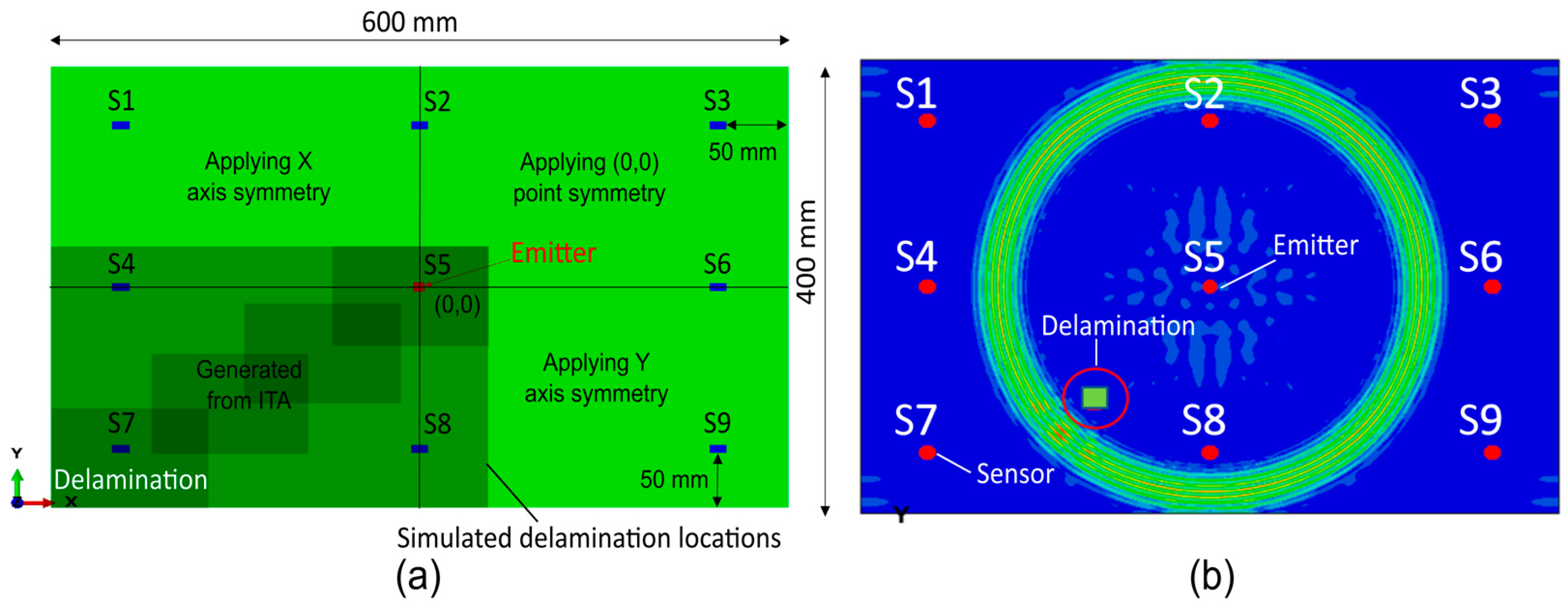
The specimen used for the study was selected according to common material and stacking used for aircraft composite components and requirements in the aerospace industry. A 600 mm × 400 mm × 3.864 mm Carbon Fiber-Reinforced Polymer (CFRP) rectangular plate was modeled with eight 14 mm × 7 mm PZT-5A sensors positioned 50 mm from the plate edges, serving as receivers, oriented symmetrically in a ¼ geometry (Figure 1a). A central 7 mm × 7 mm × 0.3 mm PZT-5A transducer acted both as emitter and receiver. An excitation signal of five sinusoidal cycles, 150 kHz frequency and 40 volts peak-to-peak amplitude with Hanning windowing was used for the ultrasonic guided wave inspection. Delamination damages were introduced as a disruption in the continuity of the FE mesh in the middle section of the plate inside the area delimited by the defect size.

Figure 1.
Simulated specimen. (a) Plate geometry, sensors network and delamination locations. (b) Simulation of a UGW propagation: out of plane displacement results with sensors network in red and its enumeration in white, and the delamination represented by a surrounded square.
A Design of Experiments (DoEs) was defined to generate a sufficiently large and representative dataset of UGW signal time series by varying defect position and size. The first set of simulations varied only the delamination position, producing 1617 cases with a fixed defect size (0.12 m × 0.08 m) and x/y position increments of 0.005 m. The second set of simulations varied in terms of both the defect position and size, yielding 1275 cases across three size groups (0.09 m × 0.06 m, 0.06 m × 0.04 m, 0.03 m × 0.02 m), with x/y position increments of 0.01 m in each group. In both sets, the defect position was limited to one-quarter of the plate, as indicated in Figure 1. Data augmentation techniques were applied, taking advantage of the symmetric configuration of the sensor network by mirroring the defects into the three remaining quadrants.
All simulations were run on an HPC server (Xeon Gold 6245, 36 CPUs, 3.1 GHz). Five CPUs per simulation were allocated (one for the implicit solver and four for the explicit solver), amounting to a total computation time of 244 h. The computation time depended on the software version used, the domain size, and the mesh element size, among other aspects. The simulations were carried out with the aim of creating a database that would be sufficient to train a deep neural network for predicting structural damage in aircraft laminates. Looking at the results obtained in this study, the authors consider that 244 h of total computation time is an acceptable time. Each simulation generated nine time series corresponding to the signals from nine sensors.
3. Data Processing and Feature Engineering
Effective data manipulation is fundamental in machine learning, as it enables raw data to be transformed into formats that allow models to extract latent, meaningful insights that are otherwise obscured. The dataset employed in this study comprises time series of ultrasonic signals. To facilitate machine learning model training, a feature engineering pipeline to transform these time series into a tabular format, where each row represents a distinct time series from the original dataset, was implemented. The transformation process consisted of five well-defined stages, as outlined below:
- Signal smoothing via interpolation: To reduce noise and enhance signal quality, an interpolation-based smoothing technique was applied. This step ensured that spurious fluctuations were minimized, allowing for more accurate subsequent feature extraction.
- Pristine signal subtraction: The second step involved subtracting a pristine reference signal from each time series. This allowed us to isolate variations of interest that are critical for understanding deviations from the baseline signal behavior.
- Windowing and computation of sum of squares: In the third stage, each time series was partitioned into five equally spaced windows. For each window, the sum of squares was calculated, providing a measure of energy within each segment. This step captured variations in signal intensity across different time intervals.
- Fast Fourier transformation (FFT) and normalization: Fast Fourier transformations (FFTs) were then applied to each windowed segment, converting the signal from the time domain to the frequency domain. To ensure comparability across different signals, the resulting FFTs were normalized to unity. This enabled the process to focus on the relative distribution of frequency components rather than their absolute magnitudes.
- Calculation of normalized FFT sum of squares: In the final step, the sum of squares of the normalized FFT values for each time window was computed. This step provided a quantitative summary of the frequency-domain characteristics of the signals, further enriching the feature set with frequency-based insights.
This structured, multi-stage feature engineering process allowed the extraction of meaningful and diverse signal characteristics, both in the time and frequency domains. By transforming the data in this manner, the resulting features retained the essential properties of the original ultrasonic signals while enhancing their suitability for machine learning model development.
3.1. Signal Smoothing via Interpolation
In this step, a one-dimensional interpolation in the time domain of the ultrasonic signals was employed. A primary advantage of this interpolation is that it aligns the signals within a unified time domain, ensuring that all signals in the dataset are equally spaced and of uniform length.
Moreover, interpolation generates intermediate data points, effectively increasing the volume of data available for model training. This augmentation can be particularly valuable when working with limited or sparse datasets, as it enhances the statistical robustness of the features. Additionally, the interpolation process contributes to smoothing the signal by mitigating fluctuations induced by noise, a common artifact in real-world data acquisition.
The importance of noise reduction cannot be overstated, especially when dealing with experimental data as opposed to simulated signals, which are often noise-free. By applying interpolation, the impact of these inherent irregularities was minimized, allowing for a more accurate representation of the underlying signal dynamics and improving the overall quality of the dataset (Figure 2).
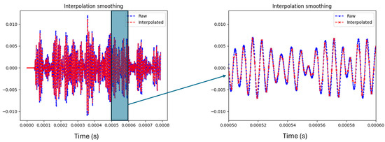
Figure 2.
Raw signal vs. interpolated signal in original view and zoomed in.
3.2. Pristine Signal Subtraction
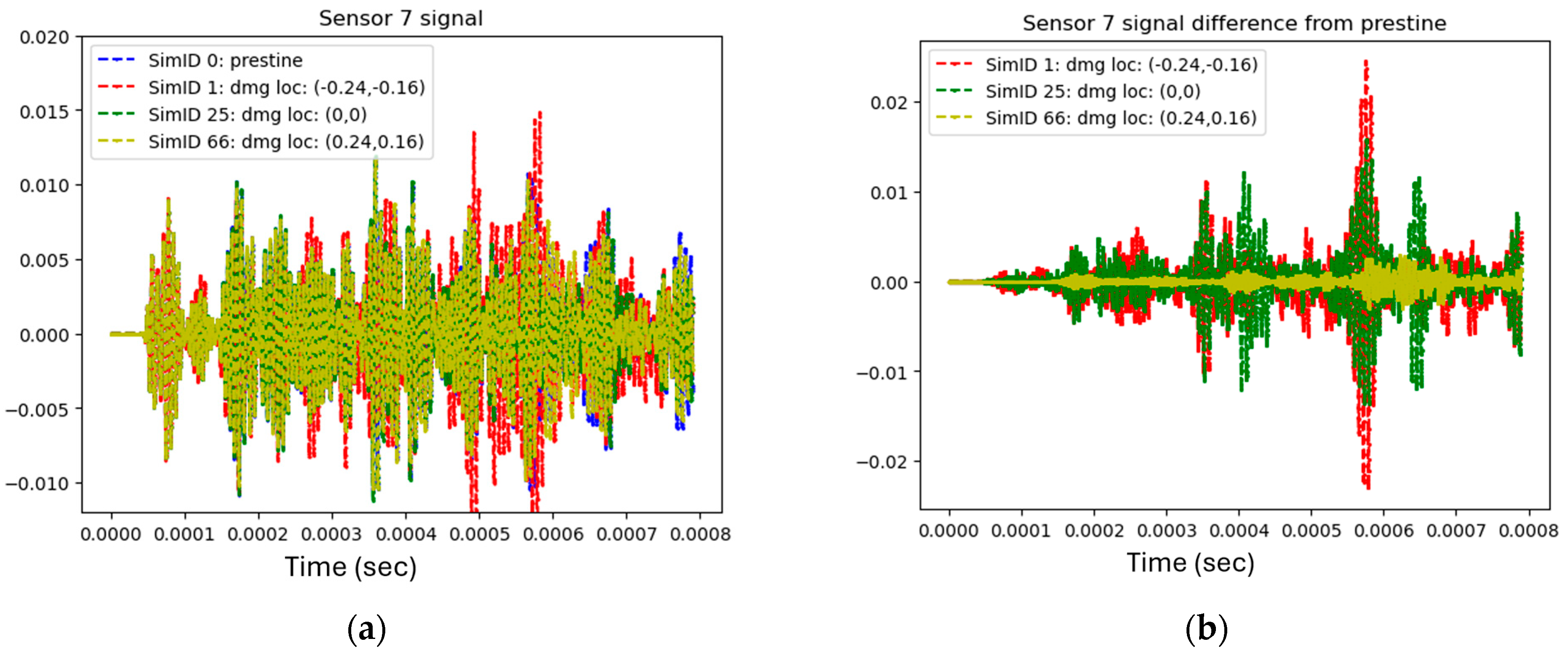
The pristine signal refers to the baseline signal generated in the absence of any damage, serving as a benchmark for comparison against damaged states. In this dataset, the raw sensor signals are very similar across simulations, regardless of whether damage is present at different locations or if the pristine (undamaged) state is simulated. While the most noticeable differences in the raw signals occur when damage is located directly beneath a sensor, the overall signal patterns remain quite comparable, making it challenging to identify and distinguish between various damaged locations using raw data alone.
To address this limitation, a pristine signal subtraction technique was implemented. By subtracting the pristine signal (zero damage) from the raw signals obtained from damaged scenarios, the areas where deviations appeared due to the presence of damage were pinpointed. This approach highlights the specific regions where damage impacts the signal, effectively enhancing the contrast between different damaged locations.
As shown in Figure 3, the differences in damage location are not readily apparent in the raw signal. However, after subtracting the pristine signal, the resulting signals exhibit much greater variation, making the differences between them more pronounced.
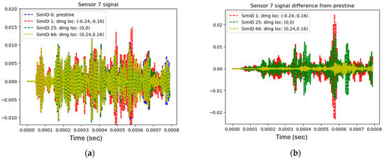
Figure 3.
Simulations from different damage locations. (a) Raw signal of simulations of different damage. (b) Raw signal subtracted with the pristine signal for the same simulations.
3.3. Windowing and Computation of Sum of Squares
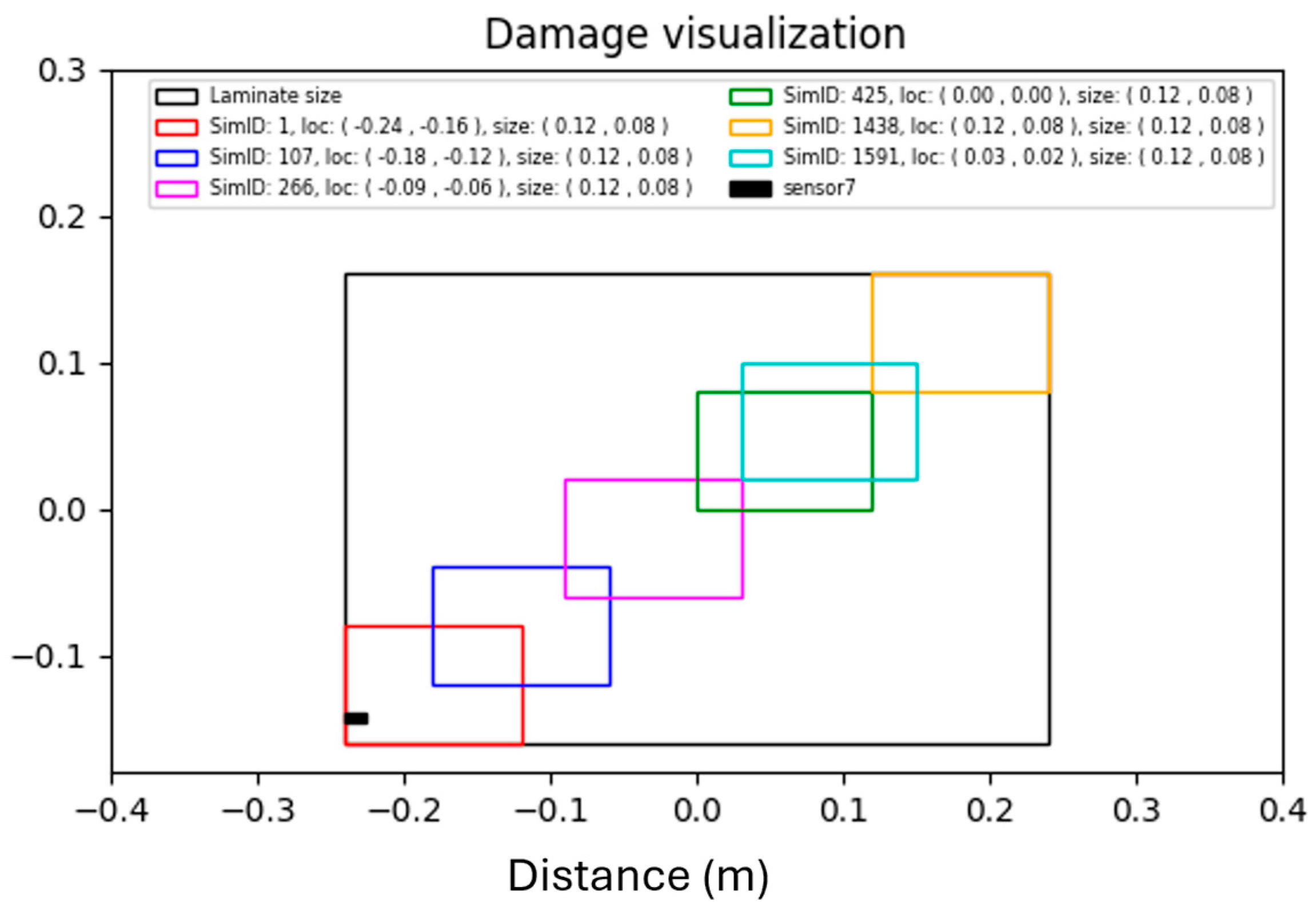
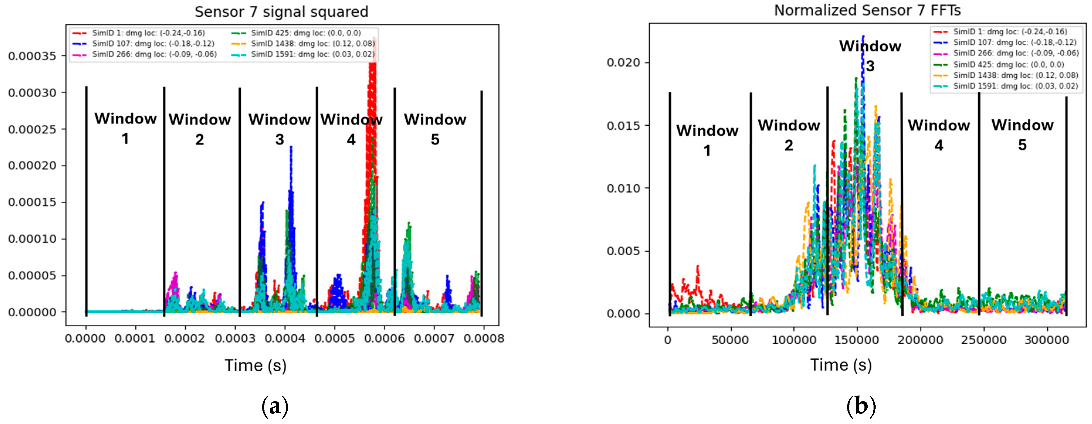
The signals were divided into five equally spaced time windows, and for each window, the sum of squares was calculated. The partitioning and computation were performed because, in some cases, the location of the damage (Figure 4) relative to the sensor was strongly correlated with the energy deposited in each time window. Figure 5 shows the raw signals from six different simulations, each represented by a different color, along with the corresponding damage size and location. It can be observed that in window 4, the signal in red corresponds to damage located at the bottom of the laminate, while in window 3, the signal in blue corresponds to damage to the bottom left of the laminate.
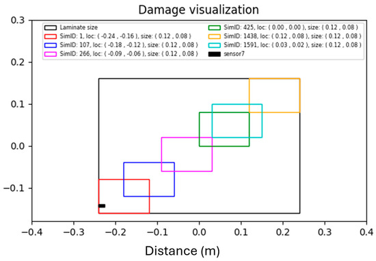
Figure 4.
The corresponding locations and size of the raw signals.

Figure 5.
Signals of different sizes and locations. (a) Raw signals of six different simulations. (b) FFTs of different sizes and locations.
3.4. Fast Fourier Transformation (FFT) and Normalization
Fast Fourier Transforms (FFTs) were applied to the signals to convert them from the time domain to the frequency domain. For each window, the resulting FFT distributions were normalized to unity, ensuring that emphasis was placed on the differences in their shapes. This normalization was crucial because “tails” appear in the frequency domain that are influenced by both the location and size of the damage, as illustrated in Figure 5b.
3.5. Calculation of Normalized FFT Sum of Squares
The sum of squares was computed for the normalized FFTs in each window. This summation of the squared frequencies represents the energy stored in the transformed signal. By calculating this for each window, meaningful features are generated, which machine learning models can more easily extract and utilize to capture relevant information.
3.6. Zero Simulation Sensor
The training dataset consists of simulations that involve damage. Consequently, training a machine learning model solely on this dataset would result in a model that cannot detect cases where no damage is present, since such instances were not included during training. To address this issue, an artificial sensor representing zero damage was created. For each location available in the original dataset, a corresponding pristine simulation datapoint was added. However, during the feature engineering process, through the substruction of the pristine simulation data, for each location, Gaussian noise was introduced to represent instances of zero damage.
4. Model Training and Validation
After data preprocessing and feature engineering, each simulation is represented by a single row with 90 columns. This includes the sum of squares computed for signals from nine sensors, each split into five windows, as well as the sum of squares for the normalized FFTs from the same nine sensors, also split into five windows. The target variables for the model are the coordinates x, y, representing the damage location and the size of the damage. The constructed model is a deep learning neural network with linear layers, which takes 90 features as input and predicts four target variables. The loss function used was Mean Squared Error (MSE) between the true and predicted values for both damage location and size. Additionally, an Adam optimizer with a learning rate scheduler was employed to gradually reduce the learning rate as training progressed, aiming to find the global minimum of the optimization function. An early stopping technique was implemented to halt the training process when performance metrics stopped improving after several epochs.
The dataset was split into three subsets: training, validation, and test sets. The training set was used exclusively for model training, while the validation set was employed for hyperparameter tuning. The test set was reserved for evaluating the model’s performance on unseen data and assessing its robustness.
To assess the performance of the developed model, the Euclidean distance was used to evaluate both the damage location and damage size. Additionally, a custom metric called the Overlap Percentage (OP) was developed to measure the overlap between the predicted damage size and the true damage size. The analytical form of this metric is given in Equation (1):
The Overlap Percentage metric ranges from 0 to 1, where values close to 1 indicate a perfect prediction, values greater than 0 indicate a good prediction, and a value of 0 could either represent a poor prediction with no overlap or a prediction that is adjacent to the true area but does not intersect with it.
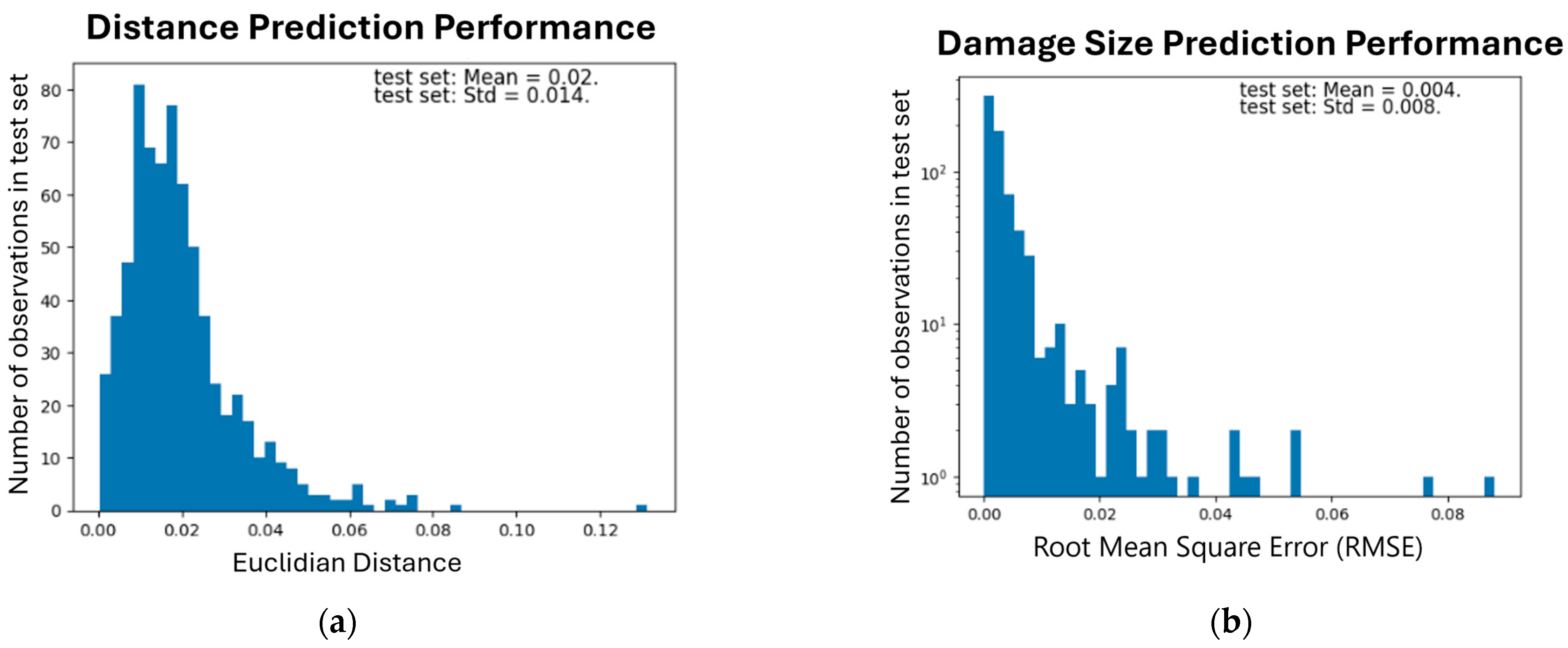
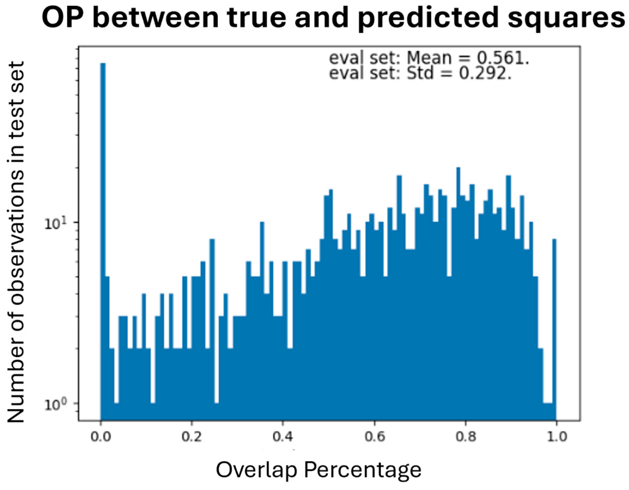
The model’s performance on the test set is visualized in Figure 6. From the left figure, it is evident that the distribution of the predictions is right-skewed and close to zero, indicating that the model accurately predicts the location of the damage. Similarly, the distribution of the predicted damage size is also right-skewed and close to zero. Regarding the OP metric, for 90% of the observations, the OP is above zero, while for the remaining cases, it is zero, as shown in Figure 7, suggesting that the location of the predictions and the true values overlap.

Figure 6.
Distributions of performance metrics. (a) Euclidian distance between the true and predicted damage locations. (b) Root Mean Square Error (RMSE) between true and predicted damage size prediction.

Figure 7.
Distribution of Overlap Percentage metric for the test set.
A second DoE was defined to assess the soundness of damage location algorithms under signal perturbations caused by operating conditions. Using 20 °C as the reference temperature and a fixed defect size of 0.12 m × 0.08 m, 42 simulations were conducted to generate a dataset, covering six temperature variations (±2, ±5, ±10 °C from the reference) at five defect positions plus a baseline condition without damage. The temperature variation was accounted for in the simulations as a change in the material properties of the composite laminate. This dataset was used exclusively for validation and not for training.
The model demonstrates good accuracy in predicting both the damage location and size, indicating that the engineered features exhibit robustness to this type of noise. Finally, the OP distribution had a mean of 0.78, indicating significant overlap between the predictions and the true values. Figure 8 illustrates the distribution of Euclidean distances for both damage size and damage location.
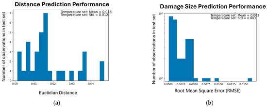
Figure 8.
Distributions of performance metrics on dataset of varied temperature. (a) Euclidian distance for the damage location. (b) Root Mean Square Error (RMSE) between the true and predicted damage size.
Author Contributions
Conceptualization, D.K, J.M.R., A.C.-E., V.T.-L. and E.K.; methodology, D.K., J.M.R., A.C.-E.; software, D.K., V.T.-L. and J.M.R.; validation, D.K., J.M.R., V.T.-L. and A.C.-E.; formal analysis, D.K., J.M.R. and A.C.-E.; investigation, D.K., J.M.R., J.H.-O., V.T.-L. and A.C.-E.; resources, D.K., J.M.R. and A.C.-E.; data curation, D.K., J.M.R. and A.C.-E.; writing—original draft preparation, P.K., J.H.-O., V.T.-L. and A.C.-E.; writing—review and editing, A.C.-E. and E.K.; visualization, P.K., D.K., J.M.R., J.H.-O. and A.C.-E.; supervision, A.C.-E. and E.K.; project administration, A.C.-E. and E.K.; funding acquisition, E.K. All authors have read and agreed to the published version of the manuscript.
Funding
“New end-to-end digital framework for optimized manufacturing and maintenance of next generation aircraft composite structures (GENEX)” was funded by the European Union under Grant Agreement No. 101056822. The views and opinions expressed are, however, those of the author(s) only and do not necessarily reflect those of the European Union or HADEA. Neither the European Union nor HADEA can be held responsible for them.
Institutional Review Board Statement
Not applicable.
Informed Consent Statement
Not applicable.
Data Availability Statement
Data are contained within the article.
Conflicts of Interest
The authors declare no conflict of interest.
References
- Perfetto, D.; Rezazadeh, N.; Aversano, A.; De Luca, A.; Lamanna, G. Composite Panel Damage Classification Based on Guided Waves and Machine Learning: An Experimental Approach. Appl. Sci. 2023, 13, 10017. [Google Scholar] [CrossRef]
- Sattarifar, A.; Nestorović, T. Emergence of Machine Learning Techniques in Ultrasonic Guided Wave-Based Structural Health Monitoring: A Narrative Review. Int. J. Progn. Health Manag. 2022, 13. [Google Scholar] [CrossRef]
- Schnur, C.; Goodarzi, P.; Lugovtsova, Y.; Bulling, J.; Prager, J.; Tschöke, K.; Moll, J.; Schütze, A.; Schneider, T. Towards Interpretable Machine Learning for Automated Damage Detection Based on Ultrasonic Guided Waves. Sensors 2022, 22, 406. [Google Scholar] [CrossRef] [PubMed]
- Nerlikar, V.; Mesnil, O.; Miorelli, R.; d’Almeida, O. Damage detection with ultrasonic guided waves using machine learning and aggregated baselines. Struct. Health Monit. 2024, 23, 443–462. [Google Scholar] [CrossRef]


Disclaimer/Publisher’s Note: The statements, opinions and data contained in all publications are solely those of the individual author(s) and contributor(s) and not of MDPI and/or the editor(s). MDPI and/or the editor(s) disclaim responsibility for any injury to people or property resulting from any ideas, methods, instructions or products referred to in the content. |
© 2025 by the authors. Licensee MDPI, Basel, Switzerland. This article is an open access article distributed under the terms and conditions of the Creative Commons Attribution (CC BY) license (https://creativecommons.org/licenses/by/4.0/).