Dynamic Modeling of Fuel Cells for Applications in Aviation ^†

Abstract

In the development of more electric aircraft, hydrogen powered fuel cells are one possible solution to progress towards emission reductions in aviation. Currently, there are numerous concepts for integrating fuel cells into future aircraft. The goal of this work was to develop a dynamic fuel cell model for simulations of the powertrain. The Modelica language together with the ThermoFluidStream (TFS) library from the German Aerospace Center (DLR) provided a suitable framework. The fuel cell model takes into account the electrochemical as well as thermodynamic behavior. Hence, the proposed multi-physics model allows simulating the whole fuel cell system, from the hydrogen tank to the electric grid. Under certain simplifications, this enables performing mission simulations of the complete powertrain of future aircraft. As such, polymer electrolyte membrane (PEM) fuel cells and solid oxide fuel cells (SOFC) were considered. The fuel cell models are checked for plausibility in a simple test case against data from the literature. Furthermore, two setups of possible applications are introduced: one for each fuel cell type, which come from two projects. The preliminary control systems of these architectures are presented. Afterwards, the first results of the fuel cell systems are discussed. These results show that the models ran robustly in various environments and operational states. They provided the desired accuracy to predict the behavior of a fuel cell, while maintaining low CPU times and being capable of enabling real-time simulations in the future.

1. Introduction

It is well-known that there has been a necessary push towards using less emissions in aviation to reduce its climate impact. Largely, this endeavor is approached by introducing alternative fuels, as well as more electric aircraft. Hereby, fuel cells can play a significant role, especially when powered by hydrogen, which eliminates CO₂ emissions. As indicated by [1,2], fuel cells could be especially applicable in a mild hybrid configuration as an auxiliary power unit (APU) or in regional aircraft as the main power source for propulsion. There have already been many studies on the component level of fuel cells, such as [3,4]. Additionally, some literature has focused on overall aircraft design (OAD) [1].

However, it is of great interest to understand the dynamic interaction of the components and subsystems in new powertrain architectures for future aircraft. A very detailed, steady-state study at a fuel cell system level was performed in [5], including an analysis on fuel cell stack sizing, considering the balance of plant components. However, there is little research to be found on dynamic system simulations. The latter go hand in hand with the development of a control scheme for the considered powertrain architectures. To progress towards both of these goals, gate-to-gate mission simulations can be carried out covering different flight phases. This is achieved at a fuel cell system level in this work. The term system in this case includes a simple version of the hydrogen supply and the air supply, as well as a thermal management system and a control logic.

As a framework, the Modelica environment is chosen, together with the in-house, open-source ThermoFluidStream (TFS) library by the German Aerospace Center (DLR). In the TFS library, there are already physics-based models for thermodynamic components such as compressors, turbines, valves, etc. However, one crucial element for performing the abovementioned multi-domain simulations is the fuel cell, which is not included in the TFS library. Hence, the goal of this work is to develop a physics-based fuel cell model that is able to connect the thermodynamic domain with the electric domain. As well as adhering to the aforementioned aspects of sufficiently low computational effort and high accuracy, another aspect of a fuel cell model is robustness in a wide application range. This will be achieved for the two most popular and most-researched types of fuel cells. One is the polymer electrolyte membrane (PEM) fuel cell, with studies concerning PEM in aviation such as [6,7]. The other is the solid oxide fuel cell (SOFC), where [8] gave a good overview of studies.

In this work, the modeling method is presented, first for the mutual parts of the two types of fuel cells, and subsequently the for type-specific aspects. Afterwards, an exemplary application is shown for each type of fuel cell, represented by one project each. A mission simulation of each fuel cell system is carried out and the results are discussed. Therefore, the focus lies on the proof that the fuel cell model is capable of running dynamic multi-domain simulations over a whole flight mission.

2. Fuel Cell Modeling

This section focuses on the methodology for modeling the two fuel cell types, following the TFS approach. For a better understanding, the TFS approach is discussed briefly, before presenting the two models. Although from an operational point of view, the PEM and SOFC differ widely, from a modeling perspective, especially at the fidelity level which is considered in this work, there are many common aspects. The latter are shown in the first subsection, covering the main thermodynamic properties and the electrochemical governing equations. Afterwards, the type-specific aspects are discussed for each model, which mainly include the mass balance and the electrochemical parameters. Additionally, the characteristics of each model are shown and compared to characteristics from the literature for a first verification of the models.

2.1. Common Modeling Aspects

When modeling physical systems, it is common practice to select two main variables: a flow and a potential variable. In the Modelica standard library, the flow variable for fluid flows is the mass flow and the potential variable is chosen as the static, thermodynamic pressure of the fluid as it drives the mass flow. This often leads to nonlinear equation systems, especially in larger simulation models, which are difficult to solve and often not very robust to simulate. One approach to tackle this problem was introduced by the TFS library, which considers a variable referred to as inertial pressure as the potential variable. After some derivation, this variable can be denoted as

$$\Delta r={\displaystyle \frac{d\dot{m}}{dt}}{\displaystyle \frac{\Delta s}{A}}$$

(1)

for the simple case of a straight pipe where $\dot{m}$ is the mass flow through the pipe, $\Delta s$ the length of the pipe and A the cross-sectional area. Thereby, the thermodynamic state is decoupled from the mass flow, which results in few to zero nonlinear equations and to more robust models than those of the Modelica standard library [9].

As a first attempt, the fuel cell was modeled completely arithmetically. This led to nonlinear equation systems, which were not robustly solvable. Therefore, as a second attempt, a volume was introduced for each electrode; i.e., more states were introduced. This allowed for a less strict coupling of the different mass flows into and out of the electrodes. Hence, the nonlinear equation system was much smaller and more robust to solve. To account for the interaction between the diffusional mass flow to the membrane and the mass flow of the consumed reactants, an additional state, the reactant concentration at the membrane, is introduced. The diffusional mass flow is then calculated according to Fick’s law of diffusion [10]. For now, the concentration of water as the product is not yet considered thermodynamically. However, it is indirectly included in the concentration loss, which will be discussed later in this section. Moreover, nitrogen diffusion and water backdiffusion are currently neglected. These mechanisms are mainly relevant for PEM fuel cells, where the hydrogen on the anode side becomes polluted by nitrogen and water vapor, which can diffuse through the membrane to the anode side.

The connection of the thermodynamic domain with the electric domain is realized by using Faraday’s law of electrolysis to derive the relation

$$i_{stack}={\displaystyle \frac{z_{H2}F{\dot{m}}_{H2,cons}}{\left(M_{H2}{N}_{cells}\right)}}$$

(2)

with the stack current $i_{stack}$, the amount of electrons transferred per hydrogen molecule $z_{H2}$, the Faraday constant F, the molar mass of hydrogen $M_{H2}$, and the number of cells $N_{cells}$. It should be noted that the number of cells is included as the mass flow of consumed hydrogen ${\dot{m}}_{H2,cons}$, evaluated for the whole stack and not for each cell individually [11,12].

To calculate the cell voltage $U_{cell}$, the thermodynamic potential, referred to as the open-circuit voltage $U_{OCV}$, has several voltage losses subtracted

$$U_{cell}=U_{OCV}-{\eta }_{act}-{\eta }_{ohm}-{\eta }_{con}$$

(3)

which are the activation loss ${\eta }_{act}$, the ohmic loss ${\eta }_{ohm}$, and the concentration loss ${\eta }_{con}$. The open-circuit voltage is assessed using the Nernst equation

$$U_{OCV}=E_0-c_T(T-T_0)-{\displaystyle \frac{RT}{2F}}·ln\left({\displaystyle \frac{p_{H2O}}{p_{H2}\sqrt{p_{O2}}}}\right)$$

(4)

with the the average stack temperature T and the normalized pressures p of water vapor, hydrogen, and oxygen, and several constants, which are the standard potential of the oxygen hydrogen reaction $E_0$, a temperature coefficient $c_T$, the reference temperature $T_0$, the universal gas constant R, and the Faraday constant F. Thus, the temperature term was added according to [11] to account for the high temperatures occurring in the SOFC. The activation loss is derived from the simplified Butler–Volmer equation as

$${\eta }_{act}={\displaystyle \frac{RT}{{\alpha }_{c}2F}}·ln\left({\displaystyle \frac{j}{j_0}}\right)$$

(5)

which mainly depends on the current density j. Additionally, the activation loss is parameterized by ${\alpha }_c$ and $j_0$, which are shown in

Table 1. Table of parameters which are used to adjust the fuel cell model to the corresponding application, where the major parameters for sizing the fuel cell stack are the number of cells and the active cell area. The membrane electrode assembly is referred to as MEA.

Symbol	Description	Unit	Mainly Affects
$N_{cells}$	Number of cells	-	Cell voltage
$A_{cell}$	Active cell area	m2	Current
$w_{mea}$	Width of the MEA	m	Volume of the MEA
$alph{a}_c$	Charge transfer coefficient	-	Activation loss
$j_0$	Exchange current density	A/m2	Activation loss
$ASR$	Area specific resistance	$\mathrm{\Omega }$ m2	Ohmic loss
$c_{con}$	Concentration loss coefficient	V	Concentration loss
$j_{lim}$	Limit current density	A/m2	Concentration loss

.

The ohmic loss is calculated by

$${\eta }_{ohm}=ASR·j$$

(6)

with the area specific resistance $ASR$ described in Table 1. This parameter is defined differently for each fuel cell type, and kept constant for now. In the future, however, $ASR$ should depend on the relative humidity in the case of a PEM fuel cell and on the temperature in the case of a SOFC. Lastly, the concentration loss is simplified compared to most literature, e.g., [13], to the relation

$${\eta }_{con}=c_{con}·ln\left({\displaystyle \frac{j_{lim}}{j_{lim}-j}}\right).$$

(7)

This is done as it is unlikely that the fuel cell will be operated near the limit current density. The parameters $c_{con}$ and $j_{lim}$ are shown in Table 1.

At a stack level, outside of the fuel cell model discussed here, pipe losses are considered by including the flow resistances of the TFS. Furthermore, a thermal capacity represents the thermal mass of the stack while connected to the fluid volumes of the electrodes. These components can be sized accordingly. Additionally, the parameters of the fuel cell stack presented in Table 1 can be adapted, e.g., to adjust the power level or the efficiency, which is influenced by the different voltage losses. Included in this table is a parameterization of the membrane electrode assembly (MEA) to specify its fluid volume, which further affects the diffusive mass transport.

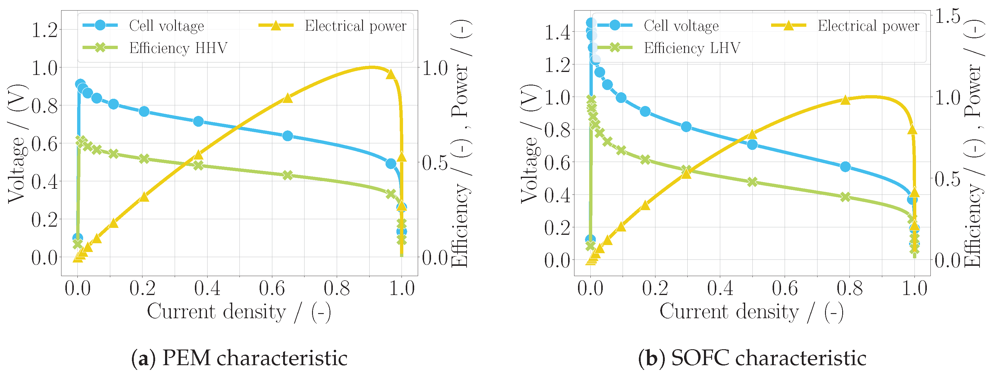
2.2. Type-Specific Models

The specific models of the two fuel cell types include the custom mass balances of the electrode volumes, since these depend on the location at which the water is produced, which differs. Additionally, the parameters of the voltage losses are defined individually. With the models being complete in regard to the equation system, a simplistic simulation was performed, where the current density was increased over the simulation time from zero to the value of $j_{lim}$ by increasing the electric power. From this simulation, the characteristics of each fuel cell type could be obtained, which are shown in Figure 1, including the voltage, the efficiency, and the normalized power output over the normalized current density. The efficiency of the PEM fuel cell was calculated using the higher heating value of hydrogen $HH{V}_{H2}$, assuming that the water was obtained in liquid form, as this is common practice when analyzing PEM fuel cells. The efficiency of the SOFC was calculated with the lower heating value $LH{V}_{H2}$, assuming that the water was obtained as vapor, due to the high temperatures. The calculation for the cell efficiency ${\eta }_{cell}$ follows the equation

$${\eta }_{cell}={\displaystyle \frac{P_{el,cell}}{{\dot{m}}_{H2,cons}·xH{V}_{H2}}}$$

(8)

with the electrical power output of the fuel cell $P_{el,cell}$, the consumed mass flow ${\dot{m}}_{H2,cons}$ and a placeholder for the corresponding heating value of hydrogen $xH{V}_{H2}$.

The polarization curve, i.e., the voltage over the current density, is depicted with the typical distribution for the fuel cell. While the voltage and the efficiency of the fuel cell simultaneously decreased over the current density, the output power increased before the concentration losses took over and ultimately all three quantities came to zero. When comparing this characteristic to more accurate models, including test data such as [14] for the PEM fuel cell and [13] for the SOFC, the good alignment of this polarization curve can be seen. This yields a first verification of the models developed in this work. Only in the case of the low current densities in the SOFC model was the voltage calculated too high, which was due to the simplification and the chosen parameterization of the activation loss. This is not considered a problem, since the current densities in aircraft applications are generally higher. Although a validation of the model is to be carried out in the future, the goal of the model is not to represent a specific fuel cell stack but rather to incorporate a general fuel cell behavior. If desired by the user, it could be parameterized to better match experimental data.

3. Applications in Aviation

In this chapter, one application is given for each fuel cell type, represented by one research project each. Both of the projects aim to analyze a powertrain of future aircraft, while also developing a control scheme. A brief overview of the architecture of the proposed powertrains is given, together with a first simple simulation setup of the fuel cell system. With this setup, an aircraft mission simulation was carried out. Hence, exemplary results of those simulations are discussed. However, the main goal of this chapter is not a detailed analysis of the systems but rather to show that the fuel cell model is capable of running in a multi-domain dynamic simulation environment for the duration of a whole aircraft mission.

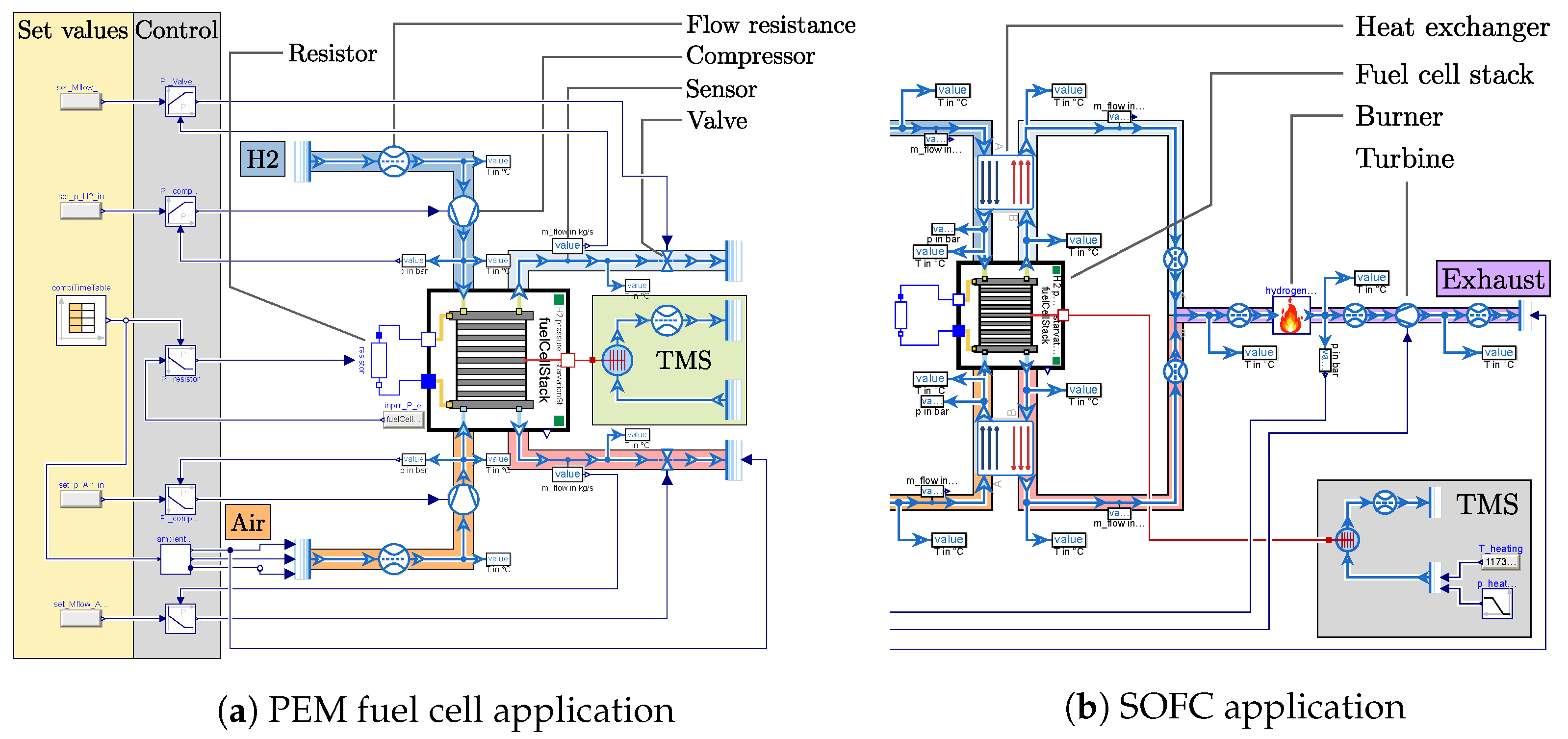
3.1. Project AMBER–PEM Fuel Cell

The PEM fuel cell model was exemplarily applied within the EU Clean Aviation project AMBER. This project focuses on demonstrating technology for a next-generation propulsion system for regional aircraft. The goal is to combine a MW class turboprop engine with a MW class PEM fuel cell system, reaching a hybridization rate of 50%. In a first step, a very simple version of the fuel cell system was modeled, without considering many subsystems such as the power electronics, the preconditioning of the reactants, and the recirculation of hydrogen. This was done as a starting point to run the fuel cell model combined with a simple control scheme over a whole aircraft mission. With this setup, computing times as low as 2 s could be achieved for a simulated mission time of 17,000 s. The simulation model is presented in Figure 2a using components from the TFS library.

The hydrogen path is marked by a blue envelope, where gaseous hydrogen is provided by a fluid source. The compressor is controlled to supply the desired pressure level for the fuel cell inlet. Behind the outlet of the fuel cell a valve is used to control the mass flow, before leading to a fluid sink, which would be the exhaust when speaking about an aircraft, thus neglecting a recirculation of the unused hydrogen, which is widely considered. Marked in orange and red is the air path, which is built the same as the hydrogen path, using a compressor for the pressure control and a valve for the mass flow control. In this simple configuration, it was found that the control can also be flipped, using the valve for controlling the pressure and the compressor for controlling the mass flow. This will be considered in the SOFC application in the following section. The electrical power of the fuel cell is regulated by adjusting a variable resistor. The thermal management system (TMS) is currently modeled ideally, to keep the stack temperature at a constant temperature. As mentioned above, mission simulations of this model were carried out for an arbitrary mission of a turboprop aircraft. The input variables were the electrical power of the fuel cell stack and the altitude. Considering the international standard atmosphere (ISA) [15], the altitude was used to calculate the ambient temperature and pressure, which was fed to the air source and sink. Here, only the static pressure at the inlet was considered, thus neglecting the dynamic part of the total pressure for now.

First results of the mission simulation are depicted in Figure 3, with the electrical power $P_{el,stack}$ as control input. Additionally, the total chemical power is shown, which is calculated by

$$P_{ch}={\dot{m}}_{H2,cons}·HH{V}_{H2}$$

(9)

similarly to the denominator in Equation (8). In blue, the net usable electric power $P_{net}$ of the fuel cell system is shown, which is the electric power of the stack subtracted by the sum of the power of the compressors $P_{compressor,i}$:

$$P_{net}=P_{el,stack}-\sum _{i=1}^2{P}_{compressor,i}=P_{el,stack}-P_{BoP}.$$

(10)

In this simple case, the sum of the compressor power can be expressed as the balance of plant power $P_{BoP}$. It can be seen that, especially in high-altitude conditions, the difference between the stack power and net power increases, meaning that the balance of plant power is higher. In high-power conditions, the stack efficiency is lower, resulting in the chemical power and the electrical power diverging. As can be seen in Figure 3, the stack efficiency defined as

$${\eta }_{stack}={\displaystyle \frac{P_{el,stack}}{P_{ch,stack}}}$$

(11)

is further evaluated in Figure 4 alongside the system efficiency

$${\eta }_{sys}={\displaystyle \frac{P_{net}}{P_{ch}}}.$$

(12)

Here, it is shown more clearly that the efficiencies decrease in high-power conditions. Additionally, they diverge in high-altitude conditions, accordingly with the power distribution.

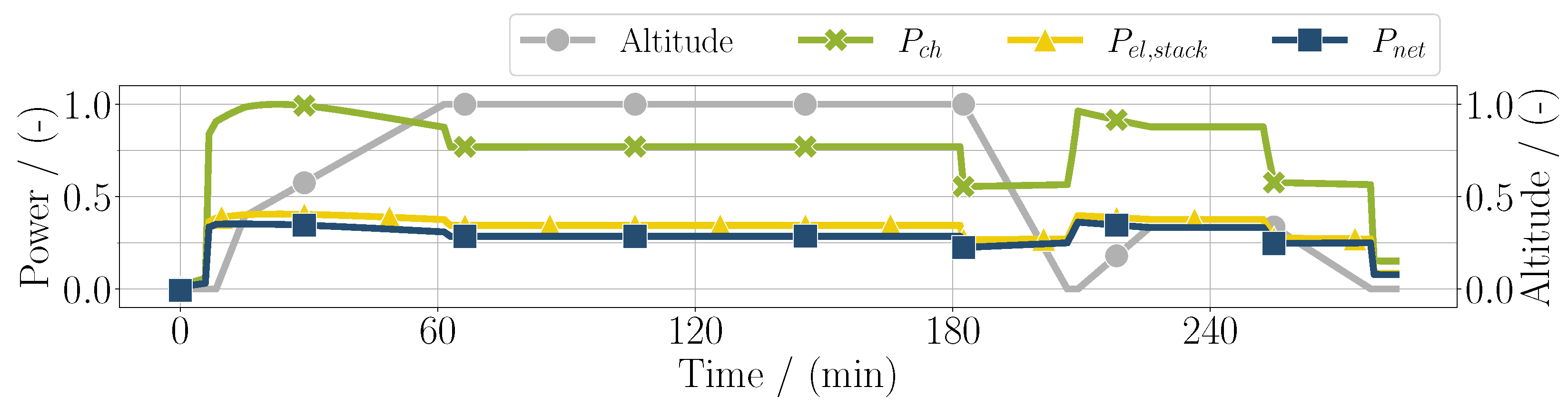
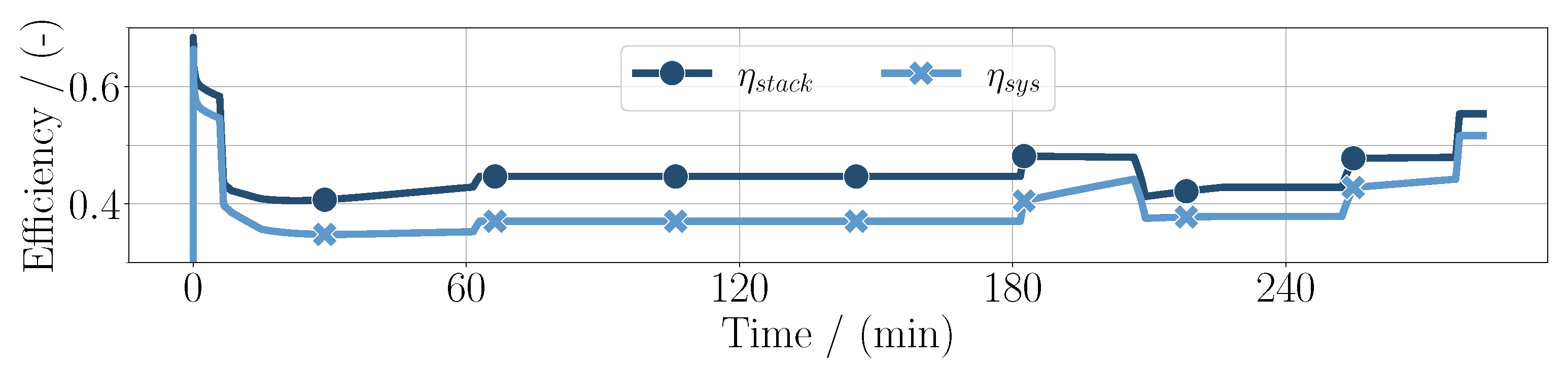
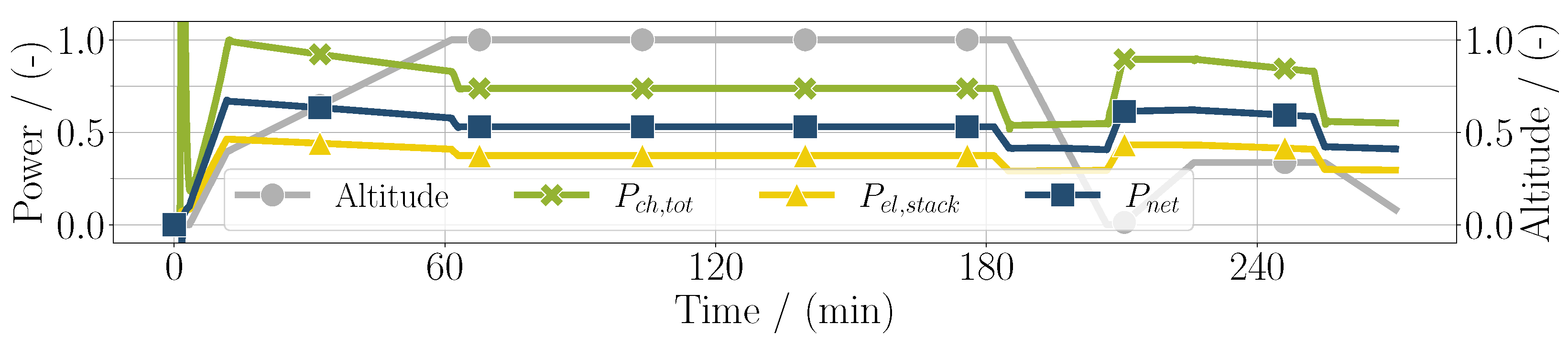
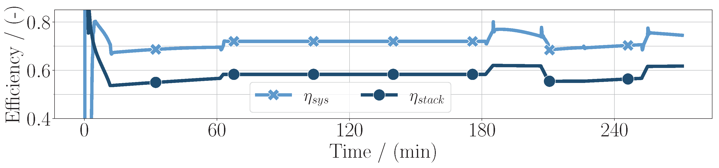
3.2. Project H2EAT–SOFC

The application for the SOFC model is the DLR-internal project H2EAT, considering a 2 MW class fuel cell system powering the complete propulsion. This is an early stage research project that focuses on the comparison between a fuselage-integrated and a nacelle-integrated concept, outlining advantages and disadvantages of each concept [16]. Similarly to the methodology described for the AMBER project, a simple architecture was modeled, to run simulations over the whole mission duration using a preliminary control system. The simulation setup, as depicted in Figure 2b, looks similar, with two major differences besides using an SOFC stack.

One difference with the PEM application is that two heat exchangers are introduced to condition the reactants. The other difference is that the two outlet gas streams of the stack are combined to burn the residual hydrogen in a combustion chamber. A turbine is then used to recuperate some of the heat energy from the combustion. In this architecture, it makes sense to use the aforementioned flipped control. Hence, the compressors are used to control the mass flow, while the turbine is used to control the pressure level. The advantage is that the pressure on both electrodes of the fuel cell is automatically almost the same. The TMS in this case is mainly included to compensate for a missing temperature control. The latter is not included, since this work focuses on fuel cell modeling.

The distributions of the electric power of the stack, the total chemical power, and the net power are presented in Figure 5. Here, the total chemical power was calculated with the mass flow of hydrogen being consumed by the stack and the burner combined. Additionally, the lower heating value of hydrogen was used for the calculation, as the water was assumed to be completely vaporized due to the high temperatures. Due to an artificially added overshoot at the beginning, which was needed to start the simulation, the chemical power was initially higher. Therefore, a more realistic maximum value was manually chosen. Since the turbine added to the net usable power output by partly recuperating the heat energy of the combustion, the latter was higher than the electrical power of the stack with the current assumptions for the compressor and the turbine efficiency. Although this needs further evaluation, the expectation is for the balance of plant power to be at least greater than zero, i.e., the power needed for the compressors can be compensated by the turbine.

Because of this power distribution, the system efficiency in this case was higher than the stack efficiency as presented in Figure 6. This is a great advantage over many PEM fuel cell systems, although the SOFC is currently too large and too heavy for an application in aviation.

4. Conclusions

The goal of building a fuel cell model for a PEM fuel cell and an SOFC, to perform dynamic mission simulations of a fuel cell system has been achieved. Although the models have not been validated yet, the comparison with more detailed studies from the literature yielded a first verification. The fidelity level was kept quite low, to enable fast computing times of less than 10 s for 17,000 s of simulated mission time on a personal computer. The models ran robustly in multi-domain simulations over a complete aircraft mission using a preliminary control scheme. This was applied in two exemplary systems, one for each fuel cell type. Although a detailed analysis was not the focus of this work, the first results of the applications show a plausible behavior for the fuel cell model.

References

1. Atanasov, G.; Wehrspohn, J.; Kühlen, M.; Cabac, Y.; Silberhorn, D.; Kotzem, M.; Dahlmann, K.; Linke, F. Short-Medium-Range Turboprop-Powered Aircraft as a Cost-Efficient Enabler for Low Climate Impact. In Proceedings of the AIAA AVIATION 2023 Forum, San Diego, CA, USA, 12–16 June 2023. [Google Scholar] [CrossRef]
2. Wehrspohn, J.; Rahn, A.; Papantoni, V.; Silberhorn, D.; Burschyk, T.; Schröder, M.; Linke, F.; Dahlmann, K.; Kühlen, M.; Wicke, K.; et al. A Detailed and Comparative Economic Analysis of Hybrid-Electric Aircraft Concepts Considering Environmental Assessment Factors. In Proceedings of the AIAA Aviation 2022 Forum, Chicago, IL, USA, 27 June–1 July 2022. [Google Scholar]
3. Salva, J.A.; Iranzo, A.; Rosa, F.; Tapia, E.; Lopez, E.; Isorna, F. Optimization of a PEM fuel cell operating conditions: Obtaining the maximum performance polarization curve. Int. J. Hydrogen Energy 2016, 41, 19713–19723. [Google Scholar] [CrossRef]
4. Calili, F.; Ismail, M.; Ingham, D.; Hughes, K.; Ma, L.; Pourkashanian, M. A dynamic model of air-breathing polymer electrolyte fuel cell (PEFC): A parametric study. Int. J. Hydrogen Energy 2021, 46, 17343–17357. [Google Scholar] [CrossRef]
5. Schröder, M.; Becker, F.; Kallo, J.; Gentner, C. Optimal operating conditions of PEM fuel cells in commercial aircraft. Int. J. Hydrogen Energy 2021, 46, 33218–33240. [Google Scholar] [CrossRef]
6. Campanari, S.; Manzolini, G.; Beretti, A.; Wollrab, U. Performance assessment of turbocharged PEM fuel cell systems for civil aircraft onboard power production. J. Eng. Gas Turbines Power 2008, 130, 021701. [Google Scholar] [CrossRef]
7. Donateo, T. Semi-Empirical Models for Stack and Balance of Plant in Closed-Cathode Fuel Cell Systems for Aviation. Energies 2023, 16, 7676. [Google Scholar] [CrossRef]
8. Fernandes, M.D.; Andrade, S.d.P.; Bistritzki, V.N.; Fonseca, R.M.; Zacarias, L.; Gonçalves, H.; de Castro, A.F.; Domingues, R.Z.; Matencio, T. SOFC-APU systems for aircraft: A review. Int. J. Hydrogen Energy 2018, 43, 16311–16333. [Google Scholar] [CrossRef]
9. Zimmer, D.; Bender, D.; Pollok, A. Robust Modeling of Directed Thermofluid Flows in Complex Networks. In Proceedings of the 2nd Japanese Modelica Conference, Tokyo, Japan, 17–18 May 2018; Modelica Conference Proceedings. Linköping University Press: Linköping, Sweden, 2008; pp. 39–48. [Google Scholar]
10. Weber, A.Z.; Newman, J. Modeling transport in polymer-electrolyte fuel cells. Chem. Rev. 2004, 104, 4679–4726. [Google Scholar] [CrossRef] [PubMed]
11. O’hayre, R.; Cha, S.W.; Colella, W.; Prinz, F.B. Fuel Cell Fundamentals; John Wiley & Sons: Hoboken, NJ, USA, 2016. [Google Scholar]
12. Wilson, J.A.; Wang, Y.; Carroll, J.; Raush, J.; Arkenberg, G.; Dogdibegovic, E.; Swartz, S.; Daggett, D.; Singhal, S.; Zhou, X.D. Hybrid solid oxide fuel cell/gas turbine model development for electric aviation. Energies 2022, 15, 2885. [Google Scholar] [CrossRef]
13. Njodzefon, J.C.; Klotz, D.; Kromp, A.; Weber, A.; Ivers-Tiffée, E. Electrochemical modeling of the current-voltage characteristics of an SOFC in fuel cell and electrolyzer operation modes. J. Electrochem. Soc. 2013, 160, F313. [Google Scholar] [CrossRef]
14. Pan, Y.; Wang, H.; Brandon, N.P. A fast two-phase non-isothermal reduced-order model for accelerating PEM fuel cell design development. Int. J. Hydrogen Energy 2022, 47, 38774–38792. [Google Scholar] [CrossRef]
15. Cavcar, M. The international standard atmosphere (ISA). Anadolu Univ. Turk. 2000, 30, 1–6. [Google Scholar]
16. Kazula, S.; Staggat, M.; de Graaf, S.; Geyer, T.; Link, A.; Keller, D.; Ramm, J.; Pick, M. Can SOFC-Systems Power Electric Regional Aircraft In 2050?—The DLR-Project H2EAT. In Proceedings of the DLRK 2024, Hamburg, Germany, 30 September–2 October 2024. [Google Scholar]
Figure 1. Characteristics of the fuel cell models in (a) for the PEM fuel cell and in (b) for the SOFC, including the polarization curve (U-j curve), the efficiency, and the electric power using the default parameterization of each model.
Engproc 90 00068 g001
Figure 2. Simulation model of the application of each fuel cell type in (a) for the EU Clean Aviation project AMBER and in (b) for the DLR-internal project H2EAT. Cut away in the visualization of (b) are the set values, the control, and the compressors, which are visually the same as in (a).
Engproc 90 00068 g002
Figure 3. Chemical power, electrical power of the fuel cell stack, and net usable power considering the balance of plant components throughout the whole mission duration for the PEM application.
Engproc 90 00068 g003
Figure 4. System efficiency and fuel cell stack efficiency throughout the whole mission duration for the PEM application.
Engproc 90 00068 g004
Figure 5. Chemical power, electrical power of the fuel cell stack, and net usable power considering the balance of plant components over the whole mission for the SOFC application.
Engproc 90 00068 g005
Figure 6. System efficiency and fuel cell stack efficiency for the whole mission duration for the SOFC application.
Engproc 90 00068 g006