Abstract
Reliable Position, Navigation, and Timing (PNT) is becoming more and more important, considering the proliferation of highly autonomous safety- and liability-critical systems. Due to their vulnerability to various threats such as deliberate Radio Frequency Interference (RFI), including jamming, spoofing, and others, there is significant research into finding backup/fallback solutions that allow safe mission completion or termination. This work compares two such systems: one based on Angle of Arrival (AoA) measurement and one based on cellular (4G and 5G) signals. The results are generated using simulations, which are substantiated by real-world performance measurements. It is shown that both systems have the potential to serve as backup navigation solutions and that the cellular system outperforms the AoA-based solution, albeit at a much higher price and with higher computational requirements.
1. Introduction
Recent years have brought significant progress in safety-critical and autonomous systems, which often rely heavily on the availability of Global Navigation Satellite System (GNSS) signals—GPS, Galileo, GLONASS, and Beidou. These signals not only provide Position, Navigation, and Timing (PNT) information but are also integral to most multi-sensor integrated navigation systems, where, integrated with an Inertial Measurement Unit (IMU), they are used for state estimation. Many such systems will fail within a very short period of time after loss of GNSS reception or try to yield control to a human operator, and while that is acceptable in some cases, this can quickly exceed tolerable risk limits for high-stakes operations (e.g., where there is a risk of injuries or monetary loss).
Despite their importance for modern technology, GNSSs are susceptible to multiple vulnerabilities. Its performance is degraded in, e.g., dense urban canyons and mountainous areas in high latitude regions. GNSS signal availability is limited in indoor environments, and the signals are also susceptible to accidental or deliberate Radio Frequency Interference (RFI), including jamming and spoofing. Clearly, for high-risk systems, it is necessary to have some resilience against GNSS outages. Many potential solutions for this problem already exist, all with their respective advantages and disadvantages. A typical disadvantage is the need to deploy dedicated additional infrastructure, such as radio transmitters.
The need to install dedicated infrastructure can be circumvented by relying on radio transmissions that are available without the user’s intervention—so-called Signals of Opportunity (SOPs). Potential signals include digital TV and radio broadcasts (DVB-T, DAB) [1], satellite constellations (Iridium-NEXT, Starlink) [2], cellular signals such as 4th-Generation Long-Term Evolution (LTE) and 5th-Generation (5G) signals [3], and others [4]. These approaches have proven to be very promising in testing [5].
The main drawback of SOP-based navigation is that the signals themselves are not optimized for navigation purposes; thus, certain limitations must be accepted. For example, the transmitter frequency and timing stability may not be controlled to a level that allows reasonable differential one-way ranging based on carrier wave cycles, simply because such close control is not necessary for its intended use case. Further complications arise if the parameters of interest are not specified or published.
The goal of this paper is to combine previous measurement and simulation campaigns by the authors to gain a comprehensive qualitative understanding of two different approaches using relatively low-cost hardware for backup navigation purposes. The simulation aspects are therefore purposefully designed to be as similar to each other as possible while still representative of the measurements and to be conservative whenever possible. However, a quantitative assessment of the performance of the system cannot be carried out with the approach chosen, since the assumptions made for this work, such as the geographical distribution of signal sources or the error characteristics of the IMU, are not necessarily representative of real-world conditions.
Previously, the authors designed and investigated a low-cost angle of arrival (AoA)-based localization system [6], which was subsequently investigated using an established in-house navigation suite [7]. Further work measured the time-domain stability of local cell towers in the vicinity of the author’s offices in Trondheim, Norway [8]. The time stability, while not representative of all potential error sources in a localization system, is a very important factor when using Time Difference of Arrival (TDOA) techniques.
2. Methodology
Using a signal for something for which it is not designed to be used implies accepting trade-offs that are caused by suboptimal signal structure as well as implementation details. Most importantly for practical reasons, the governing standards often do not specify aspects crucial to navigation, or specify them so vaguely that relying only on the standard would imply navigation performance so poor so as to be of little practical use. This is particularly true for cellular signals, as cellular communication is governed by an organically grown set of standards and regulations, with many optional features, and a conflation of terminology where, for example, “5G” is both a marketing term applied to telecommunication networks that may or may not actually be 5G networks, a broad set of technological standards defined by the 3GPP, and a more abstract idea of what the new generation of networks should achieve in terms of performance. To a user, it is virtually impossible to understand which parts of the standards and in which revision are implemented by the network operator, especially when it comes to optional features and architectural decisions that impact frequency stability.
As a preliminary step to this work, the authors investigated the time stability of real-world signals in the vicinity of Trondheim, Norway. Two of the three network operators exhibited strong time stability of the transmitter oscillators, with a peak-to-peak total clock error (i.e., combined transmitter and receiver clock error) of about 1 m to 5 m (equivalent to 3 ns to 16 ns) over a time period of one hour. The third operator exhibited stepped drift with piecewise constant drift rates of several hundred meters per hour, reinforcing the point that understanding the implementation details of the network in use is important. Thus, the reader is advised that all results derived in that work are quantitatively applicable to the measurements in Trondheim only and that care should be taken when trying to derive results for any other place.
The simulations used in [7] were used as a basis for this work. This is intended to provide a direct comparison between relatively low-cost angle of arrival and a somewhat more expensive but still affordable cellular-based system. It is assumed that the transmitter tower positions are known and that the receiver’s navigation solution has converged and is initially precisely known. The justification for the latter precondition is easy to assert: the intended use case for this navigation system is an Unmanned Aerial Vehicle (UAV) that encounters GNSS disturbances in flight and needs to gracefully end or safely abort the mission, or otherwise guide the platform out of the impacted area. The operators will simply not start the mission if initialization of the navigation platform is not possible. The former assumption is more problematic: in some countries, the positions of the cell phone towers are public information, while in others they are not. Norway concealed this information in 2022 [9]. However, even with this information not publicly known, it is possible either to estimate the transmitter position by inverting the localization problem while the UAV still has GNSS reception or to survey the area beforehand. The former solution essentially turns the navigation platform into a Simultaneous Localization and Mapping (SLAM) problem. Thus, while it clearly causes more work for the user and is overall a less desirable situation, this is not deemed a critical shortcoming.
2.1. Overview of AoA and Cellular-Based SOP Navigation
As mentioned in the introduction, there are many different approaches to exploiting radio signals for opportunistic navigation.
The previous work using the KerberosSDR [10] platform uses an antenna array and four coherent RTL-SDR receivers (RTL-SDR refers to a low-cost receiver based on a repurposed TV receiver chip, the RTL2832U). Each element receives the same signal at a slightly different time, and this can be used to estimate the AoA using established algorithms such as Multiple Signal Classification (MUSIC). This is computationally inexpensive but provides relatively low angular precision. In addition, there are non-linearities and singularities to consider. The system suffers from decreased performance with increasing range, since a constant angular measurement error provides a larger area of confidence if the range is increased. This approach is flexible with respect to the signals tracked, as long as the signal can be correctly associated with a transmitter position. The signals investigated in the previous work used the Automatic Identification System (AIS) signals. AIS broadcasts the transmitter position in a Time-Division Multiple Access (TDMA) scheme, thus allowing simple transmitter localization and AoA association.
For aiding through AoA, the measurement function important for the Error-State Kalman Filter (ESKF)—also called Multiplicative Extended Kalman Filter (MEKF)—used in this work is given by
where and are the distances from the UAV to the ith beacon to the east and north, respectively; is the current heading; and y is the resulting body-fixed bearing.
To track the cellular signals, we used STARE (real-time Software Receiver), which is an open-source project by the ESA for long-term monitoring of cellular towers that also provides the observables required for navigation. STARE tracks the epoch (time of arrival, ToA) of the Primary and Secondary Synchronization Signals (PSS and SSS, respectively) of the LTE and 5G frames [11,12]. It also tracks Doppler shift, yielding a velocity constraint along the Line-of-Sight (LoS) vector from the transmitter to the receiver. Neither the range nor the velocity constraint fundamentally decreases in performance with distance, and the measurement model, while not linear, is simpler.
For range-based aiding, the measurement model is given as
where the symbols are the same as before and is the height difference between the beacon and the UAV.
For velocity-based aiding, the measurement model is given as
where u, v, and w are the velocity components in the northward, eastward, and downward directions, respectively.
2.2. Simulated Scenario
For the previous work described in [7], a simulated flight trajectory (see Figure 1) was created using ArduPilot’s integrated flight simulator. ArduPilot was used to generate a ground truth state time series, representing a realistic flight model. From this ground truth state, the simulated measurements were derived using simple geometry.
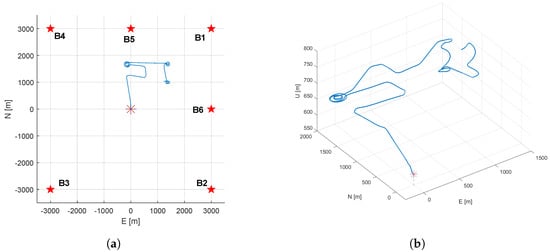
Figure 1.
Illustration of simulated scenario. (a) Top-down projection with beacons; (b) 3D representation of flight path.
2.3. Noise Model
Noise for the cellular-derived simulated measurements is assumed to be Gaussian. Gaussian noise does not capture all real-world noise effects, which are a superposition of a multitude of different influences, such as thermal noise and clock steering through feedback loops. However, over the short time frames considered for upset recovery in this work, most effects can be assumed to be static, such that the remaining randomness can be simplified to be Gaussian. To ensure a conservative estimate, the standard deviation is chosen to be much larger than experimentally encountered by the authors.
This ignores two major potential factors: a constant bias/drift and multipath. Not modeling transmitter clock drift can be justified, as the previous measurements have shown that the drift rate changes slowly enough that the changes expected over the test intervals presented here is negligible; the constant bias can be estimated while reliable GNSS reception is still available. The receiver clock error can be eliminated by monitoring multiple uncorrelated transmitter towers, ideally from different network providers.
For the purposes of this study, the noise parameters are always the same and can be found in Table 1. The values are chosen to be representative of the experimental results in [7,8]. Biases are not added. The IMU and compass measurements are not artificially corrupted, since this is not a study on the feasibility of dead reckoning. Instead, it was shown in previous works (see [7]) that the residual numerical noise and other factors are enough to induce error growth in dead reckoning integration, which causes filter divergence. Similarly, the focus of this work is not on the altitude component, and in fact, this was entirely ignored during the previous work, which is why the added noise for altitude measurements is low.

Table 1.
Noise characteristics used in simulations.
3. Results
The noise parameters used for this study can be found in Table 1. The sample rate for the AIS and cellular signals is at 1 except in the high-frequency case, where it is set to 25 in the cellular case.
In this scenario, there up to six available transmitters for all three aiding types. The transmitters are located at (3000, 3000); (−3000, 3000); (−3000, −3000); (3000, −3000); (3000, 0); and (0, 3000) , where the first number is the distance from the origin in the northward direction, while the second number is the distance in the eastward direction. All transmitters are located at 0 m altitude. The location of these transmitters is indicated in Figure 1a. For the one-, two-, and three-transmitter cases, the first one, the first and second, and the first through third are used, respectively.
Figure 2a illustrates the performance of the three investigated approaches projected into the horizontal plane. For this scenario, it is assumed that a compass measurement, an altimeter, and initial GNSS reception for the state estimates to converge are available. Unaided navigation is not shown but can be found in [7].
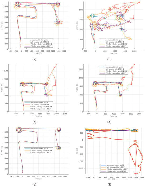
Figure 2.
Illustrations of performance (a) with six transmitters; (b) with one transmitter; (c) with two transmitters; (d) with three transmitters; (e) with two transmitters and a high sampling rate; (f) in the vertical plane, with six transmitters and no altimeter.
The advantages of the cellular approach become clearer when fewer transmitters are in use. While only one transmitter does not provide satisfactory navigation results even with the cellular approach (see Figure 2b), as few as two beacons already yield a good solution for the cellular system (Figure 2c,d), especially when used with a higher sample rate (Figure 2e, “2 B., high SR” in Table 2).
Table 2.
Error statistics (in m) for the different scenarios.
The cellular approach, due to the observability of the altitude, also clearly outperforms the AoA-based approach when no altimeter is present (Figure 2f, “6 B., no alt.” in Table 2). Since the performance of the system is virtually identical whether or not a heading sensor is available (“6 B., no comp.” in Table 2), this scenario is not included in the illustrations.
Qualitative numerical representation of these results can be found in Table 2. This table lists some error statistics of the aforementioned scenarios. At each epoch, the estimation error , where is the vector of the three-dimensional position and is the Kalman estimate, is calculated. The largest absolute error, the mean of the error, and the root mean square (RMS) of the error are presented.
4. Discussion
The results from Section 3 indicate that navigation based on cellular signals is very promising given the assumptions made there. They also indicate that the cellular system is seemingly superior to the AoA-based system. However, this does not mean that the cellular approach is superior in all regards, and a nuanced discussion about the respective advantages and drawbacks is warranted.
The simulations, while based on realistic assumptions to the best of the authors’ knowledge, also deliberately omit effects that are very hard to quantify without further investigation. The most prominent omission is that of the previously mentioned multipath effects, which are thought to be minimized by operating at altitude compared to operating at ground level, where the effects would be significant.
Similarly, the hardware requirements for the two systems are quite different. While the AoA-based system uses a KerberosSDR four-channel receiver and a Raspberry Pi 4 for processing, with a total hardware cost of approximately EUR 500, the cellular system currently requires an Ettus Research Universal Software Radio Peripheral (USRP) B200 for each tracked tower, a somewhat capable x86-based desktop PC, and potentially a highly stable rubidium oscillator. Currently, the monetary cost of this setup adds up to approximately EUR 10,000, although significant cost optimizations of the setup are possible.
4.1. Advantages of the Cellular Navigation System
In addition to its better overall navigation performance, the cellular system is much more versatile. LTE and 5G are deployed worldwide, covering most of Earth’s land area. Thus, the cellular navigation system has, in theory, the potential to work in any populated area. However, care must be taken when extrapolating the results from the previous paper [8] to other places, as the cellular parameters and key performance characteristics may vary considerably between two sites. The results from Trondheim may not be representative of the area of interest.
Cellular networks are also dense, increasing the likelihood of good geometry. They are diverse in frequency and technology, increasing resilience to accidental or deliberate attacks. Their complex signal features, while not optimized for this purpose, allow range and velocity measurements, which are much better suited to navigation than AoA measurements.
The main advantage of range and velocity measurements over AoA measurements is that in theory, they do not decrease in precision with increasing distance from the transmitter; thus, the performance of the system does not decrease if the transmitter network is less dense. The AoA-based system, on the other hand, suffers degraded performance if the beacons are far away. In addition, the propagation characteristics of the AIS signal, which uses a very low-datarate communications channel on a relatively low carrier frequency, increase the range significantly. This is desirable for its intended purpose, but it also increases the risk of unpredictable non-line-of-sight propagation paths that would be misleading if used for navigation.
The range and velocity measurements also provide information about altitude if the geometry allows it (i.e., if the flight altitude is high enough so that the slant range is appreciably larger than the projection onto a level plane). Out of practicality considerations, this is not realistically possible with the AoA-based setup. However, this will likely be of little real-world use, as barometric altimeters are cheap and precise for the time scales and geographic areas that are of interest.
4.2. Advantages of the AoA-Based Navigation System
One of the main drawbacks of the cellular navigation system is that it requires accurate knowledge about the transmitter position. Cell phone towers, however, do not broadcast their own positions. To what extent this information can be queried from other sources, such as public datasets issued by the network operators or spectrum management authorities, varies greatly from country to country. For instance, information on approved transmitter locations is public information in both Germany and Switzerland but is no longer accessible in Norway. If it is not available directly, either the towers must be localized by manual site surveys (e.g., by measuring the signal strength of visible towers using a mobile phone) or their positions must be co-estimated during the initial flight phase while full GNSS reception is still available. This is in contrast to the AIS-based system, where the transmitters send their own position estimates in the payload message, thus solving this problem.
As mentioned, this AoA system is poorly suited for three-dimensional positioning, but it does provide heading information, in contrast to the omnidirectional cellular navigation sensor. For practical uses, this is likely more valuable than altitude information: magnetic compasses have well-known limitations in certain situations, such as close to the magnetic poles, close to large amounts of magnetic material, or when the influence of on-board magnetic fields such as those from electric motors becomes significant and difficult to compensate.
4.3. Availability of Signal Sources, Sampling Rates, and Geometry
Figure 2e clearly shows that the cellular system profits from higher sampling rates, as errors average out more quickly. The same would be true for the AoA-based system, at least for constant biases and errors with a non-zero-median symmetric distribution.
However, for the AIS-based system, increasing the sample rate is not possible, as it is outside of operator control and consists of at most one sample per received AIS burst. Each vessel in range transmits one AIS burst every 2 s to 180 s; thus, the maximal sample rate is very much dependent on how many vessels are in view, what type of vessel they are, and how fast they are currently moving. In contrast, the maximal sample rate for the cellular system is much higher, and in theory, one observable could be produced for every PSS and SSS transmission for each cell in view, although a longer averaging period can have advantages as well. Additionally, a very high sample rate ⪆ 100 might also cause unacceptable computational demands.
AIS signals are broadcast on two known frequencies ( and ), which can both be received easily using a low-bandwidth radio. It is therefore straightforward to exploit all available signals, even with very low-cost hardware such as the RTL-SDR receivers. Thus, this system utilizes the available information optimally. On the other hand, the receiver requirements are much higher for the cellular system, and tracking more than one center frequency with one radio may only be possible in rare cases. Thus, for practical reasons it is currently necessary to select only a few cells, and no other available signals are exploited. In practice, this implies poor geometry and less redundancy with the current test setup.
The geometry used in this work, as illustrated in Figure 1, is meant to represent an expected distribution of available signals. Along more heavily used seaways, having several vessels geometrically spread around the vehicle seems realistic, but further investigation should consider a geometry where the vessels are all located to one side—such as when a UAV flies over the shore. For cellular networks, the geometry can vary significantly, from a multitude of towers in range in a dense urban settlement to only one tower every couple of kilometers. For the intended use case, the geometry is thus not likely to exist in this for in practice, but it is likely to be representative for this work.
5. Conclusions and Further Work
This work has shown that cellular signals of opportunity show great potential for navigation. It is superior to the AoA-based approach in performance, in the sense that it requires fewer transmitters in view and in the sense that it allows a higher sample rate with decreased noise characteristics—at the cost of a more complex and expensive system with a demand for more information to be known a priori, and potential problems caused by real-world concerns such as loss of lock. Thus, as with any system, careful consideration must be taken for the particular use case in mind.
The approach of combining real-world measurements with simulations clearly indicates that further research is required in order to achieve real-world applicability. Several further investigations are in preparation:
5.1. Acquisition of Signals and Loss of Lock
During this work, it was assumed that the tracking loops hold a continuous lock on the cellular signals. At this time, there are two problems with this assumption: First, the software (STARE) needs to be told manually which cell to track, requiring precise knowledge about the current situation. Second, the software does not handle loss of lock gracefully, sometimes causing rapid excursions of the state estimate before a fault condition is detected and the observables are discarded.
5.2. Parameter Variation
This study did not investigate the impacts of different setups, such as distance to, and number of, available signals. Further studies are planned to vary those parameters, investigating the tolerance of the two systems to variation in conditions outside of user control.
5.3. Tracking More Signals
Currently, one USRP is required per carrier frequency, even if multiple cells are available on adjacent frequencies within the available USRP bandwidth.
5.4. Clock Cost Optimization
Currently, it is assumed that a rubidium standard or other very stable oscillator is available on the vehicle. This should be redundant if enough uncorrelated signals are available, which shoud allow to compensate for the receiver clock error to some extent. While the approaches typical for GNSS receivers would not work for cellular networks, limited compensation based on statistical assumptions should be possible.
Author Contributions
Software development: A.W. and O.H.; data analysis: A.W.; original draft: A.W.; review: all authors; conceptualization and supervision: A.M. and N.S. All authors have read and agreed to the published version of the manuscript.
Funding
This research received no external funding.
Institutional Review Board Statement
Not applicable.
Informed Consent Statement
Not applicable.
Data Availability Statement
Not applicable.
Conflicts of Interest
A.W., A.M. and N.S. are employed by SINTEF Digital. O.H. is employed by the Norwegian University of Science and Technology. Except for the aforementioned employments, all authors declare that the research was conducted in the absence of any commercial or financial relationships that could be construed as a potential conflict of interest.
References
- Palmer, D. Position Estimation Using the Digital Audio Broadcast (DAB) Signal. Ph.D. Thesis, Institute of Engineering Surveying and Space Geodesy, The University of Nottingham, Nottingham, UK, 2010. Available online: https://eprints.nottingham.ac.uk/12456/1/539180.pdf (accessed on 28 July 2022).
- Neinavaie, M.; Khalife, J.; Kassas, Z.M. Acquisition, Doppler Tracking, and Positioning with Starlink LEO Satellites: First Results. IEEE Trans. Aerosp. Electron. Syst. 2022, 58, 2606–2610. [Google Scholar] [CrossRef]
- Del Peral-Rosado, J.A.; Raulefs, R.; López-Salcedo, J.A.; Seco-Granados, G. Survey of Cellular Mobile Radio Localization Methods: From 1G to 5G. IEEE Commun. Surv. Tutor. 2018, 20, 1124–1148. [Google Scholar] [CrossRef]
- Kapoor, R.; Ramasamy, S.; Gardi, A.; Sabatini, R. UAV Navigation using Signals of Opportunity in Urban Environments: A Review. Energy Procedia 2017, 110, 377–383. [Google Scholar] [CrossRef]
- Kassas, Z.M.; Khalife, J.; Abdallah, A.A.; Lee, C. I Am Not Afraid of the GPS Jammer: Resilient Navigation Via Signals of Opportunity in GPS-Denied Environments. IEEE Aerosp. Electron. Syst. Mag. 2022, 37, 4–19. [Google Scholar] [CrossRef]
- Winter, A.; Sokolova, N.; Morrison, A.; Johansen, T.A. GNSS-Denied Navigation using Direction of Arrival from Low-Cost Software Defined Radios and Signals of Opportunity. In Proceedings of the EUCASS, Lille, France, 3–8 July 2022. [Google Scholar] [CrossRef]
- Winter, A.; Sokolova, N.; Morrison, A.; Hasler, O.; Johansen, T.A. Low-cost angle of arrival-based auxiliary navigation system for UAV using signals of opportunity. In Proceedings of the 2023 IEEE/ION Position, Location and Navigation Symposium (PLANS), Monterey, CA, USA, 24–27 April 2023; pp. 1162–1169, ISSN 2153-3598. [Google Scholar] [CrossRef]
- Winter, A.; Morrison, A.; Sokolova, N. Analysis of 5G and LTE Signals for Opportunistic Navigation and Time Holdover. Sensors 2024, 24, 213. [Google Scholar] [CrossRef] [PubMed]
- Nasjonal Kommunikasjonsmyndighet. Deler av Tjenesten til Finnsenderen.no Tatt Bort. Available online: https://nkom.no/aktuelt/deler-av-tjenesten-til-finnsenderen.no-tatt-bort (accessed on 20 February 2024).
- Othernet. KerberosSDR-4x Coherent RTL-SDR. Available online: https://othernet.is/products/kerberossdr-4x-coherent-rtlsdr (accessed on 2 May 2024).
- Lapin, I.; Granados, G.S.; Samson, J.; Renaudin, O.; Zanier, F.; Ries, L. STARE: Real-Time Software Receiver for LTE and 5G NR Positioning and Signal Monitoring. In Proceedings of the 2022 10th Workshop on Satellite Navigation Technology (NAVITEC), Noordwijk, The Netherlands, 5–7 April 2022; pp. 1–11. [Google Scholar] [CrossRef]
- European Space Agency. ESA ESSR STARE. Available online: https://essr.esa.int/project/stare (accessed on 2 May 2024).
Disclaimer/Publisher’s Note: The statements, opinions and data contained in all publications are solely those of the individual author(s) and contributor(s) and not of MDPI and/or the editor(s). MDPI and/or the editor(s) disclaim responsibility for any injury to people or property resulting from any ideas, methods, instructions or products referred to in the content. |
© 2025 by the authors. Licensee MDPI, Basel, Switzerland. This article is an open access article distributed under the terms and conditions of the Creative Commons Attribution (CC BY) license (https://creativecommons.org/licenses/by/4.0/).