Abstract
Currently, the entire agricultural sector is under significant pressure. The causes that may explain this are different, such as climate change, market instability, and the decline in the population of agricultural workers. As a result, the agricultural tractor and machinery field is at the center of an intense technological revolution. One of the possible solutions to the aforementioned problems can be represented by agricultural vehicles equipped with autonomous driving systems. The key pillar of an autonomous driven vehicle is its autonomous driving algorithm which represents the link between the information coming from the vehicle’s sensor systems and the success of the vehicle’s operative mission. In this paper, an experimental assessment of the motion strategy for a four-wheel differential drive agricultural rover was conducted. This work is structured in three parts. First, the description of the working principles of the autonomous driving algorithm is proposed. Then, the case study and the scaled prototype designed for this purpose are described. In the end, the result obtained by the virtual model, which acts as reference case, is compared with the results that came out of the field test campaign. The outcomes show the overlap between the virtual and real results.
1. Introduction
In recent years, the agricultural machinery sector has been involved in an authentic technological revolution. There are several reasons linked to this phenomenon. One of the main causes is represented by climate change [1,2], since agriculture represents 11% of the total anthropogenic greenhouse gas (GHG) emissions [3]. Climate change, in its turn, is responsible for the increase in unexpected and intense weather events with unavoidable consequences for crop quality and quantity [4,5]. Also needing to be considered is the necessity of increasing food production, despite the population of agricultural workers declining [6,7], due to the actual growth trend of the world’s population [8]. In this challenging context, both the academic and industrial sectors are exploring several ways to achieve cleaner and more efficient operations in agriculture [9,10]. The consequences of these attempts are the design of agricultural vehicles equipped with innovative powertrains such as hybrid electric tractors [11,12,13], experimentation with alternative propellants [14,15], and the increasing implementation of IoT systems onboard agricultural vehicles [16,17]. In this context, agricultural robots can represent the best compromise, because they include all the aforementioned features [18,19,20]. Agricultural robots are intelligent and autonomous vehicles with a very large field of application. Indeed, they can be used in modern precision farming applications [21,22], such as monitoring field health status [23,24], or they can also perform traditional agricultural tasks like spraying or harvesting [25,26,27]. One of the most important features of these kinds of vehicles lies in their motion strategy [28,29,30].
To the authors’ knowledge, there is still a lack of understanding with respect to agricultural rovers equipped with four-wheel differential drive systems. Indeed, most of the work currently presented in the literature focuses on autonomous agricultural vehicles, operating in orchards, equipped with traditional steering systems. For example, some works focus on the optimization of steering maneuvers for front-wheel steering agricultural tractors [31,32,33,34] or on the fleet movement synchronization of tractors [35,36]. Other works focus on certain specific aspects that the autonomous tractor must consider during its mission such as fuel consumption optimization [37] or soil condition [38,39].
The aim of this work is to prove the applicability and the reliability of an autonomous driving strategy, developed in a virtual environment, for an agricultural rover equipped with a four-wheel differential drive system and operating in a vineyard/orchard environment. This paper must be considered in continuity with the work presented in [40], where the algorithm principles, developed by the same authors of this study, are described. Consequently, the proposed model would represent a powerful tool for developing control strategies for this kind of vehicle. After a description of the working principles of the autonomous driving algorithm, the case study and a scale prototype, specifically designed and assembled for this study, are described. Then, the results obtained from the virtual model are discussed and compared with the ones obtained during the field tests.
2. Materials and Methods
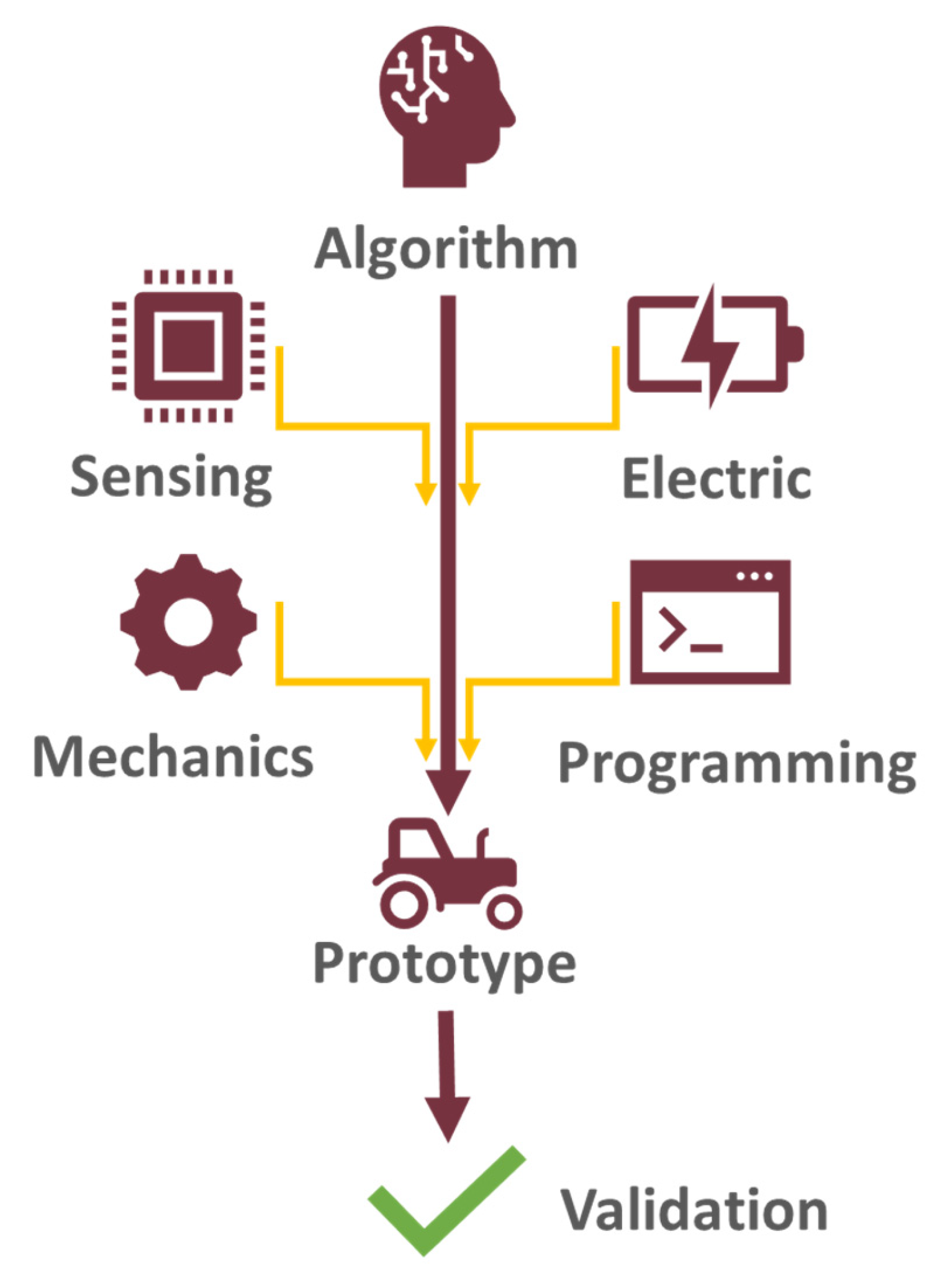
In this section, the autonomous driving algorithm and the case study under investigation are described. The flow chart of the conceptualization of this study is shown in Figure 1.

Figure 1.
Flow chart of the logic behind this study.
In particular, the autonomous driving algorithm and its execution in a virtual environment, which is taken as a reference case, represents the starting point. Then, a scale prototype, in which the algorithm can be implemented, was designed and built for this study, through a multidisciplinary approach. Then, a series of field tests were conducted in order to compare the experimental results with the modeled ones in order to eventually validate the autonomous driving model itself.
2.1. Autonomous Driving Algorithm
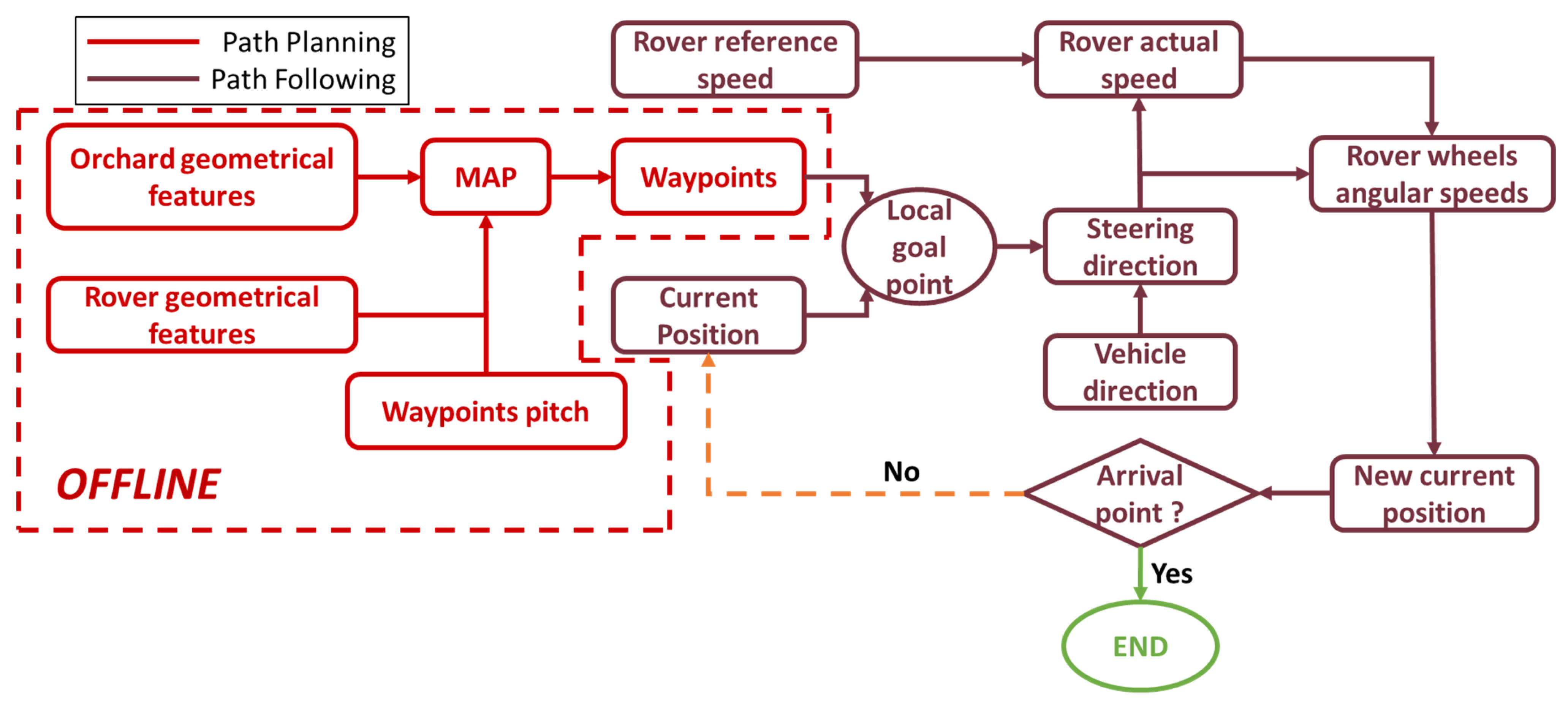
The autonomous driving algorithm is essentially made up of two main parts, as it is possible to observe in Figure 2: path planning and path following.
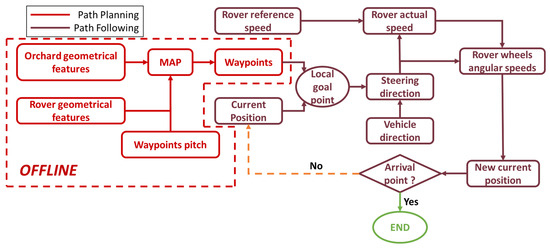
Figure 2.
Flow chart of working principles of autonomous driving algorithm.
The path-planning phase aims to define a succession of points, namely waypoints (WPs), that represent the path that the vehicle must follow in order to accomplish its mission. The motion planning process is performed in offline mode, i.e., before the vehicle’s mission starts. Once the rover’s ideal trajectory has been generated, it will be implemented in the rover control unit and used to perform the vehicle mission. The first step of the path-planning process is the reconstruction of the environment in which the rover will operate. The map consists of a matrix where only two possible values are permitted for each cell:
- 1 in the case of the presence of an obstacle;
- 0 in the case of a free path.
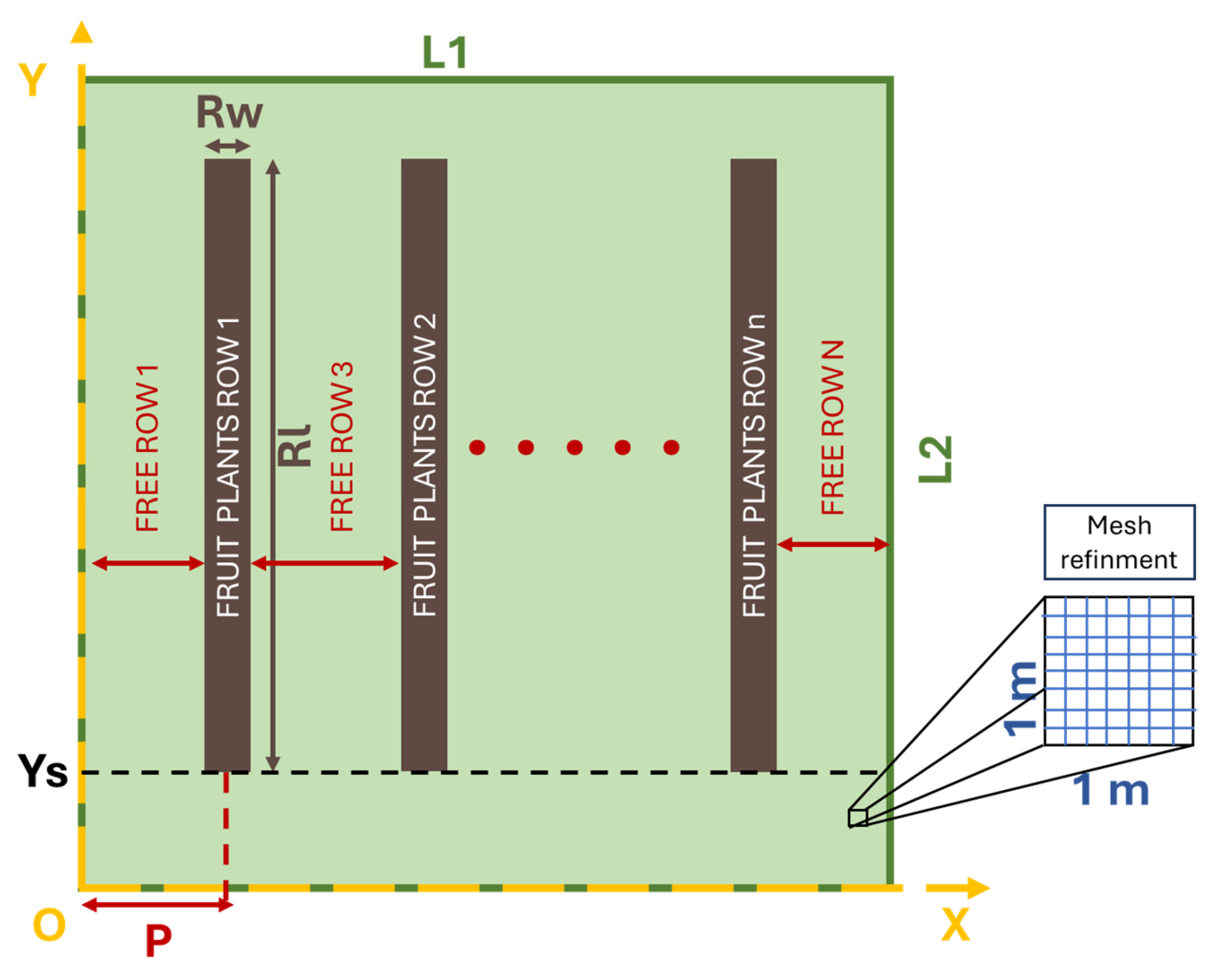
The generation of the map is managed automatically by the algorithm after the user defines several input parameters (Figure 3):
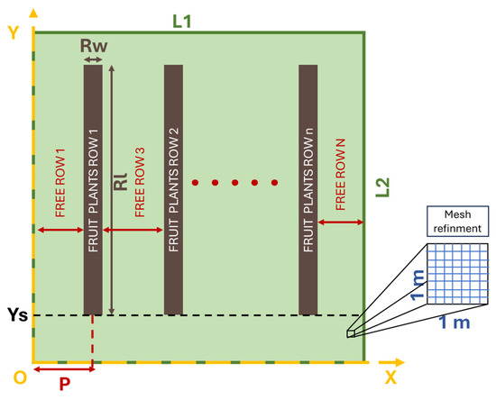
Figure 3.
Representation of the map generation input parameters.
- The number of fruit plant rows n;
- The width Rw and length Rl of fruit plant row;
- The width L1 and length L2 of the orchard field;
- The fruit plant row’s start position Ys;
- The mesh refinement m, which consists of the number of cells contained in each square meter;
- The number of free rows N = n + 1;
- The fruit plant row recurring step P = L1/N.
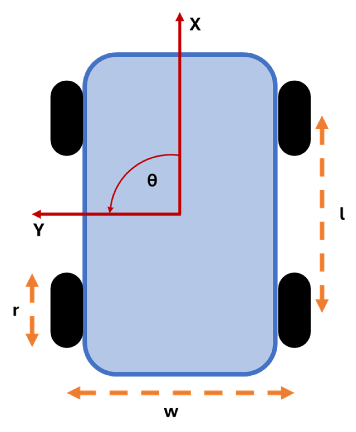
The next step, necessary for solving the motion planning process, is the definition of the input parameters related to the vehicle features. The developed algorithm is based on a 2D model; thus, the state of the vehicle is fully defined through three degrees of freedom, two translational (longitudinal X and lateral Y movements), and one rotational (yaw ϴ) around the axis perpendicular to the movement plane (Figure 4).
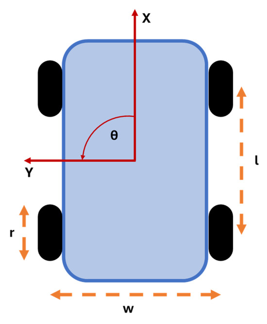
Figure 4.
Rover’s degrees of freedom (red) and its input parameters (orange).
In this regard, there are four vehicle parameters:
- Rover width w;
- Rover wheelbase l;
- Tire radius r;
- Minimum vehicle turning radius.
As can be seen, among the vehicle’s input parameters there is no information about the vehicle’s steering system. Indeed, the trajectory planned is independent of the steering system equipped on the rover, which is implemented in the path-following phase instead.
At this point, the ideal trajectory of the rover can be traced. The motion planning process is based on Dubins theory [41,42]. It consists of a geometrical planner according to which the trajectory of an object can be traced with a combination of segments and circular arcs, given a start and an arrival point and their relative orientation on the map. This kind of theory is particularly appropriate in the case of vineyards/orchards since there are mainly two kinds of trajectory executed by the rover:
- A straight line along the fruit plant row;
- Hairpin turns to go out from a free row and enter the next one.
The input variables that must be set in order to generate the planned trajectory are:
- Start and goal points and their respective orientations on the map.
- The number of checkpoints that are some known reference points through which the vehicle must pass.
- Waypoints pitch distribution (WPP), which consists of the distance between two consecutive waypoints.
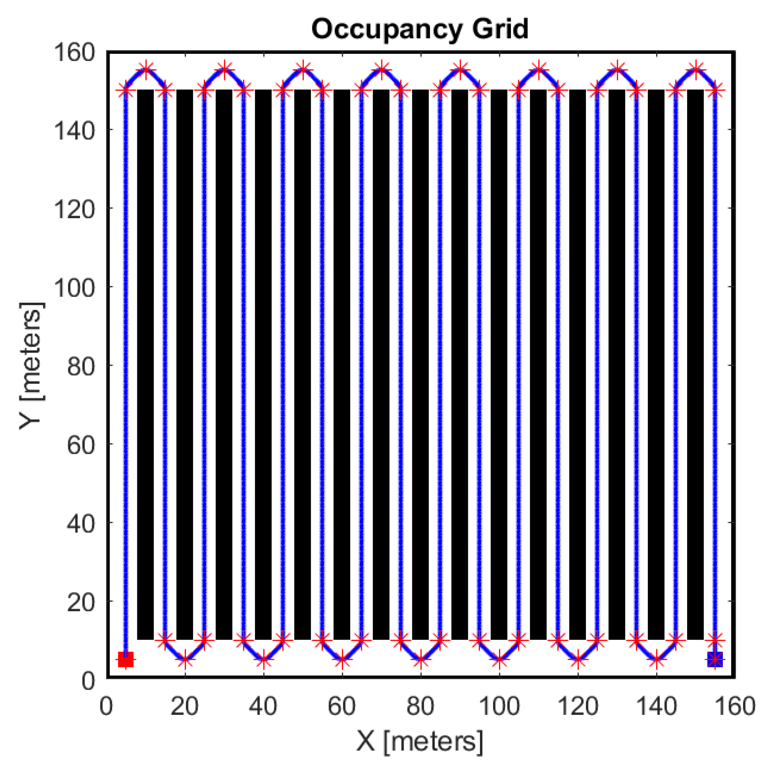
In particular, the checkpoints are inserted manually by the user. In Figure 5, an example of the results of the path-planning phase is shown.
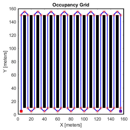
Figure 5.
Example of planned trajectory; the red stars represent the checkpoints.
The output of the path-planning phase represents the input of the path-following phase. The scope is to follow a predetermined trajectory (waypoints) adequately. The working principle of the path-following process, which is based on a pure-pursuit controller [43], is shown in Figure 6.
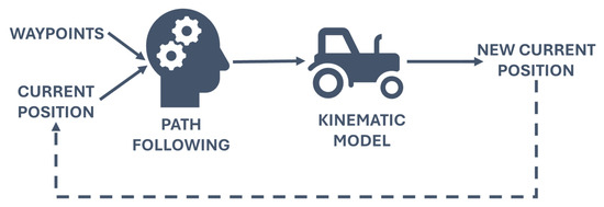
Figure 6.
Path-following working principle.
The input parameters of the path-following phase are:
- Cycle time t, which defines the time range in which the rover takes action.
- Distance threshold Dth, which represents the maximum distance below which the reference waypoint is considered reached.
- Look-ahead distance LD, which represents the radius of the circumference centered on the rover’s center of mass.
The path-following algorithm is structured in four steps. First, the algorithm identifies a local goal point (LGP), given by the intersection between the LD circumference and the ideal path (Figure 7). The LGP represents the provisional arrival point that the rover tries to reach in the cycle time considered.
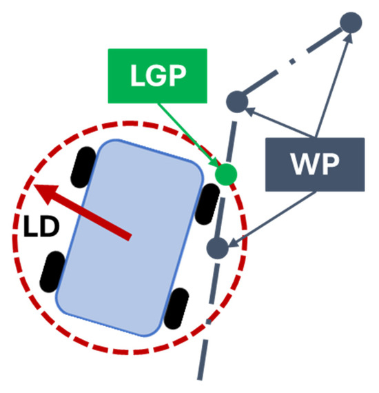
Figure 7.
Representation of LGP identification.
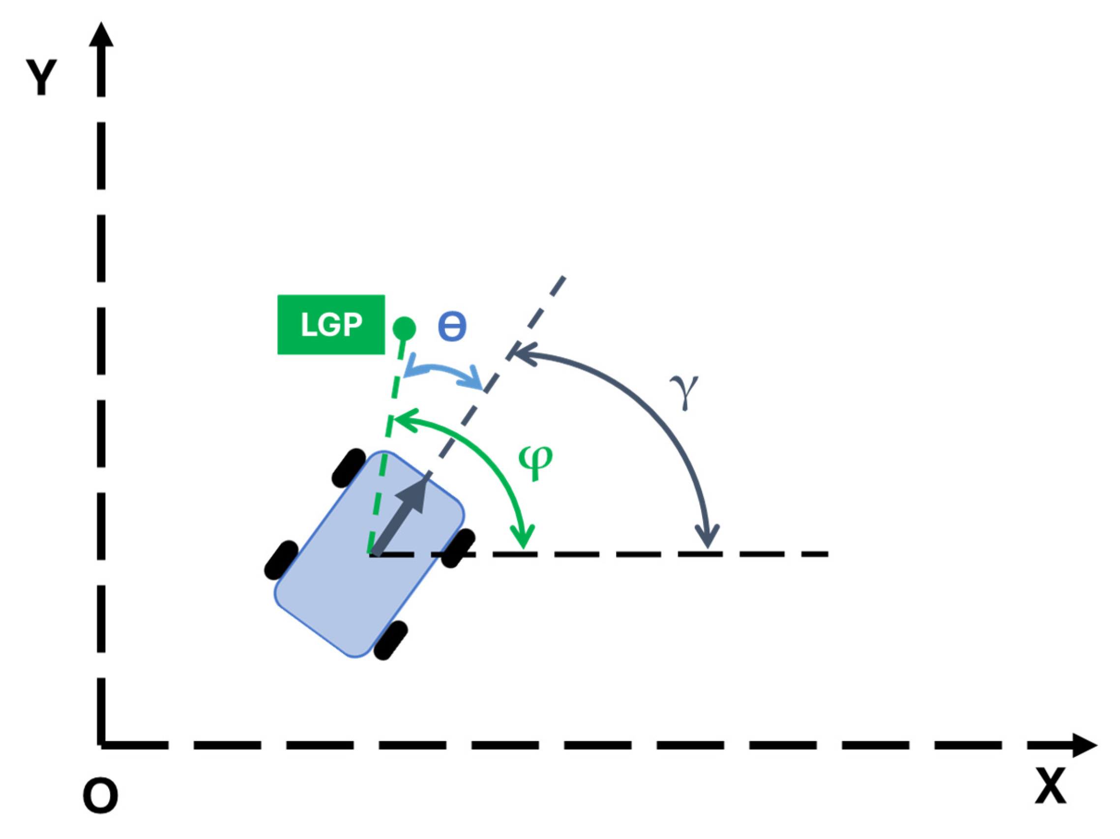
Then, the rover is able to define the LGP direction φ with respect to its position. Hence, given the rover’s orientation γ with respect to the map reference system, the algorithm calculates the yaw angle/steering angle ϴ (Figure 8) according to the following equation:

Figure 8.
Steering angle representation.
At this point, it is possible to determine the yaw speed:
The longitudinal speed v is calculated according to the following equation:
where
- vt represents the maximum rover speed;
- ϴmax is the maximum steering angle of the rover which, in this case, has been set to 360° because according to the kinematic model used the pivot maneuver is admissible.
Given the vehicle’s longitudinal and yaw speeds, the algorithm calculates the angular speeds that must be imposed on the left and right wheels, according to the differential drive kinematic model [44]:
where
- ωr/l represents the angular speeds of the right and left tires, respectively;
- v is the rover’s actual longitudinal speed;
- r is the tire radius;
- l is the rover’s wheelbase;
- represents the yaw speed.
In this way, the rover can reach the local goal point in the specific time cycle considered.
2.2. Case Study and Prototype
As stated previously, the scope of this study is the empirical assessment of an autonomous motion strategy for a four-wheel differential agricultural rover. The input parameters used in the algorithm are shown in Table 1:

Table 1.
Algorithm input parameters.
There are just two parameters that remain to be defined: the look-ahead distance LD and the waypoint pitch distribution WPP. Indeed, the aim of the virtual model is to find the best combination of these two parameters so that the rover is able to pursue the ideal trajectory in the best way possible. Both the virtual model and the simulations were carried out on MATLAB R2021b (Mathworks Inc., Natick, MA, USA). With respect to the input parameters, a scaled orchard was reconstructed (Figure 9) and a scaled prototype was designed and developed.
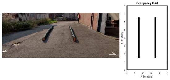
Figure 9.
Orchard replica and its virtual counterpart.
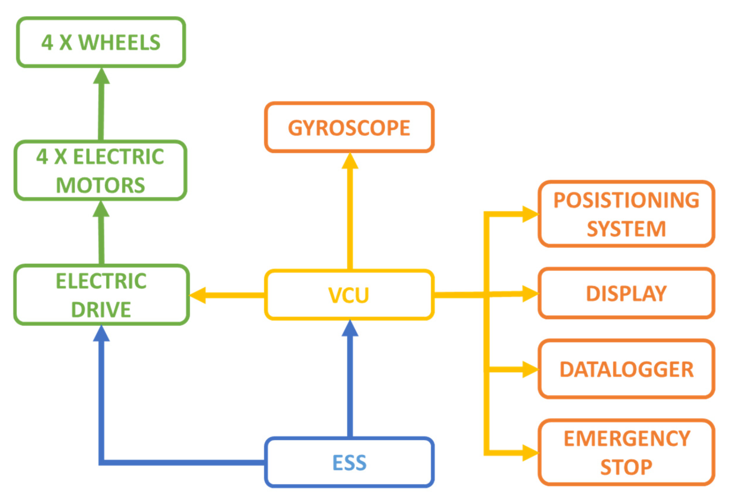
Focusing on the scale prototype, its functioning block diagram is represented in Figure 10.
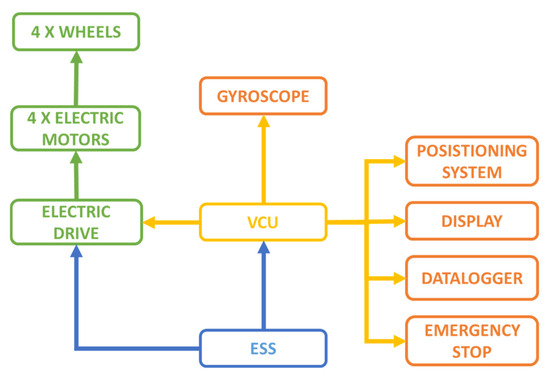
Figure 10.
Rover block diagram.
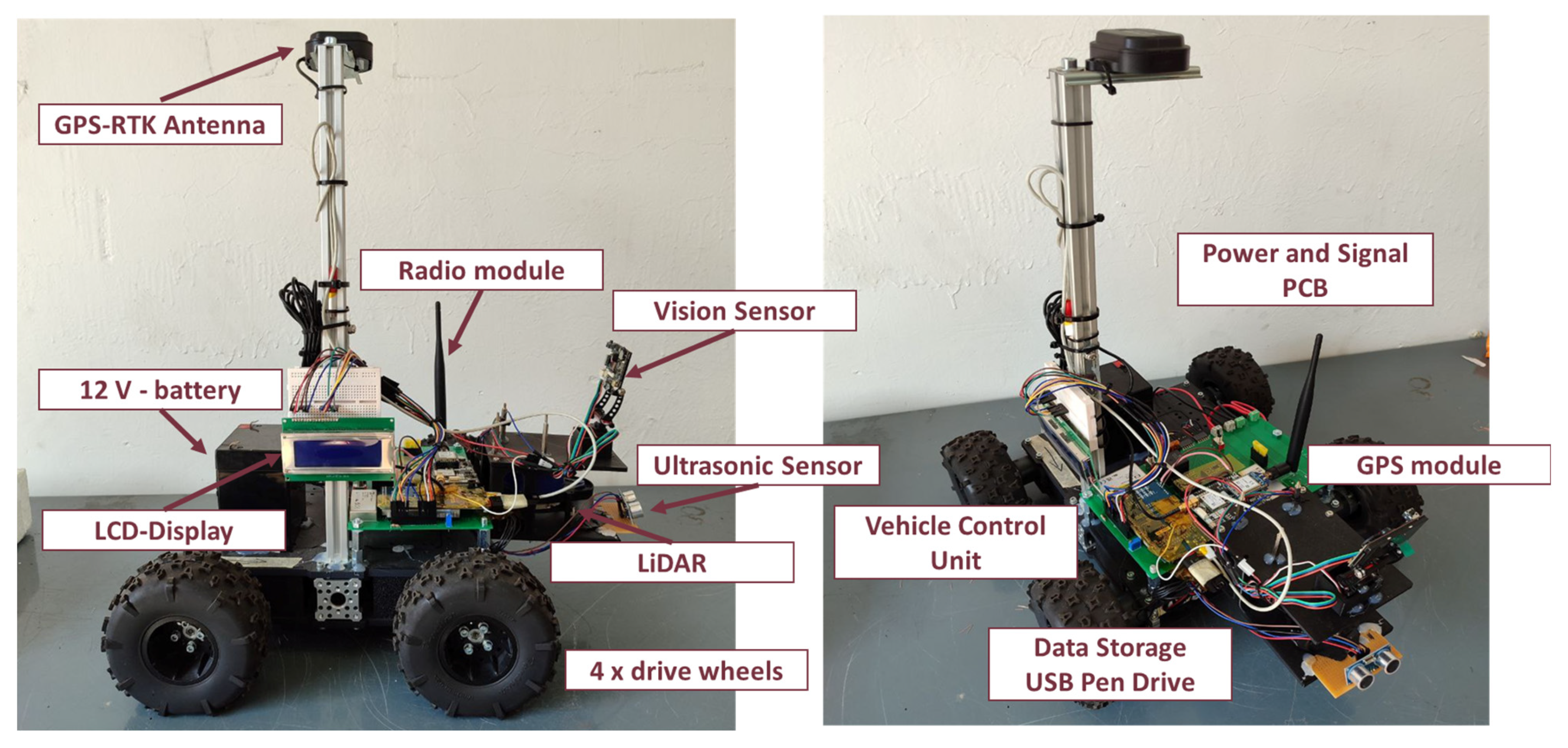
The rover is equipped with a 12 V lead-acid battery as an electric storage system (ESS). This provides electric energy both for traction and control. All the vehicle functionalities are managed by the vehicle control unit (VCU). There are several sensors connected to the VCU:
- A gyroscope sensor which is used to manage the steering angle and the vehicle’s direction on the map;
- A positioning system which is based on GPS-RTK technology that is composed of a GPS module and a radio module;
- A datalogger integrated into the VCU in order to collect all the information related to the actual status of the vehicle such as its position, direction, speed, etc.;
- A display making it possible to directly read information about the current status of the vehicle;
- LiDAR, ultrasonic, and vision sensors, which in this study are used as an emergency stop system.
The real aspect of the rover, highlighting its main components, is reported in Figure 11.
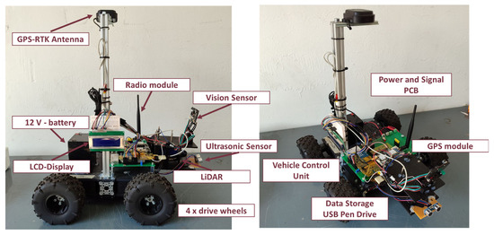
Figure 11.
Scale prototype and its main components.
3. Results and Discussion
In this section, the results obtained by the virtual model are compared with the experimental ones.
3.1. Virtual Model Results
As stated previously, once the input parameters linked to the field and vehicle characteristics have been defined, there are only two parameters that must be defined:
- Waypoint pitch distribution WPP;
- Look-ahead distance LD.
Indeed, the aim of the virtual model is to identify the best combination of these two parameters that, having fixed all the remaining variables, makes it possible to accomplish the mission of the vehicle in the best way possible. Hence, the opportunity to calibrate the algorithm virtually is a great advantage in terms of saving time and also security, because the user does not need to perform all the tuning phases in the real tests.
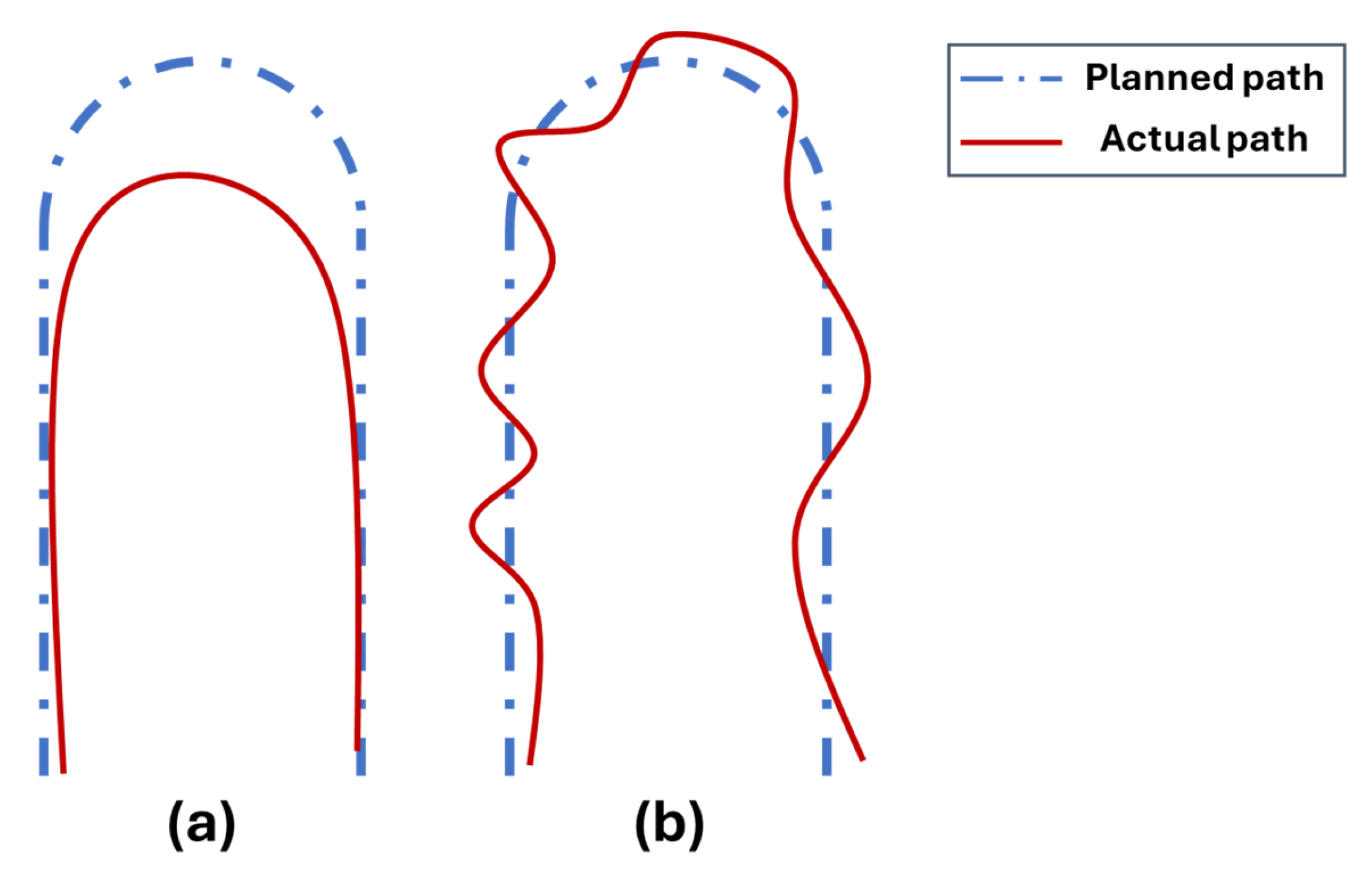
Several simulations with different values of LD and WPP were run. In particular, the LD range was varied from 0.25 to 1.2 m, whereas the WPP range was varied from 0.1 to 1 m. The aim was to avoid the rover following the planned trajectory as represented in Figure 12. All the simulations were performed using MATLAB R2021 according to the parameters defined in Table 1. Furthermore, since the simulations were run using a 2D virtual model, the following considerations were included:
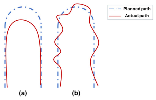
Figure 12.
Unwanted ways of path covering: (a) the rover follows the ideal path too closely; (b) the rover oscillates around the ideal path.
- The rover is completely defined with three degrees of freedom: lateral and longitudinal movements, and yaw rotation.
- The vehicle is represented as a rigid body and its wheels are in a condition of pure rolling with respect to the ground.
- The rover’s low operating speed implies that lateral slip can be ignored.
To evaluate the best possible combination of factors, the methodology defined in [40] was adopted. According to this method, the evaluation occurs through two parameters:
- The average trajectory deviation (ATD), which corresponds to the mean value of the trajectory deviation (expressed in meters) of the rover calculated for every occupied position with respect to the ideal path.
- The oscillating factor (OF), which takes into account the number of steering corrections performed by the rover to keep itself near to the ideal trajectory.
These two performance parameters are condensed into one single performance indicator, namely relative accuracy (RA), and are defined according to the following equation:
Hence, the simulation with the highest value of RA will correspond with the best combination of WPP and LD, because this means that the trajectory deviation and steering corrections are lower.
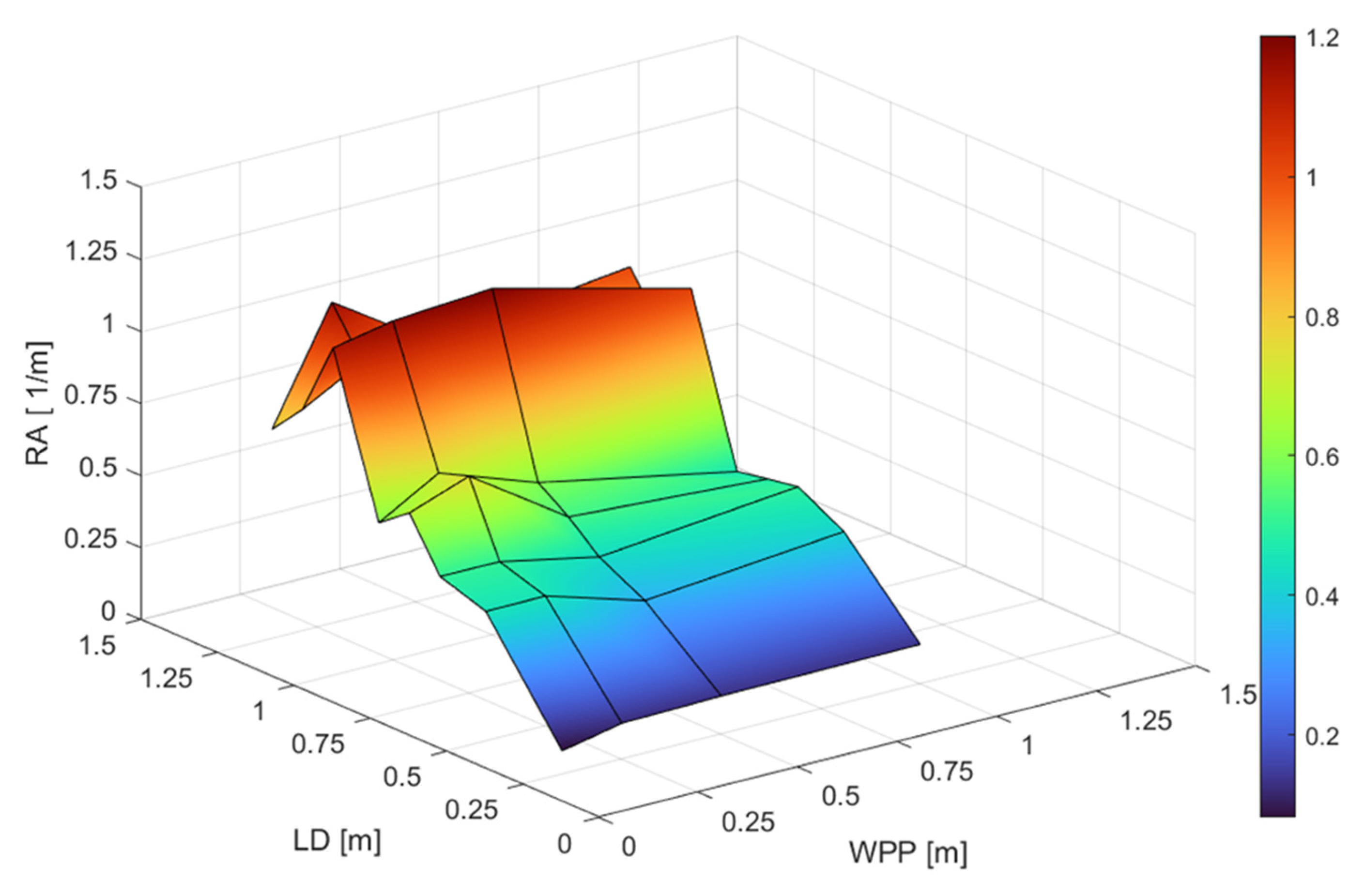
The RA trend as a function of WPP and LD is reported in Figure 13.

Figure 13.
RA surface as a function of LD and WPP.
Observing the chart, it can be noted that the best results in terms of RA occur when LD and WPP are equal to 1 m and to 0.5 m, respectively (Figure 14).
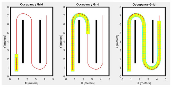
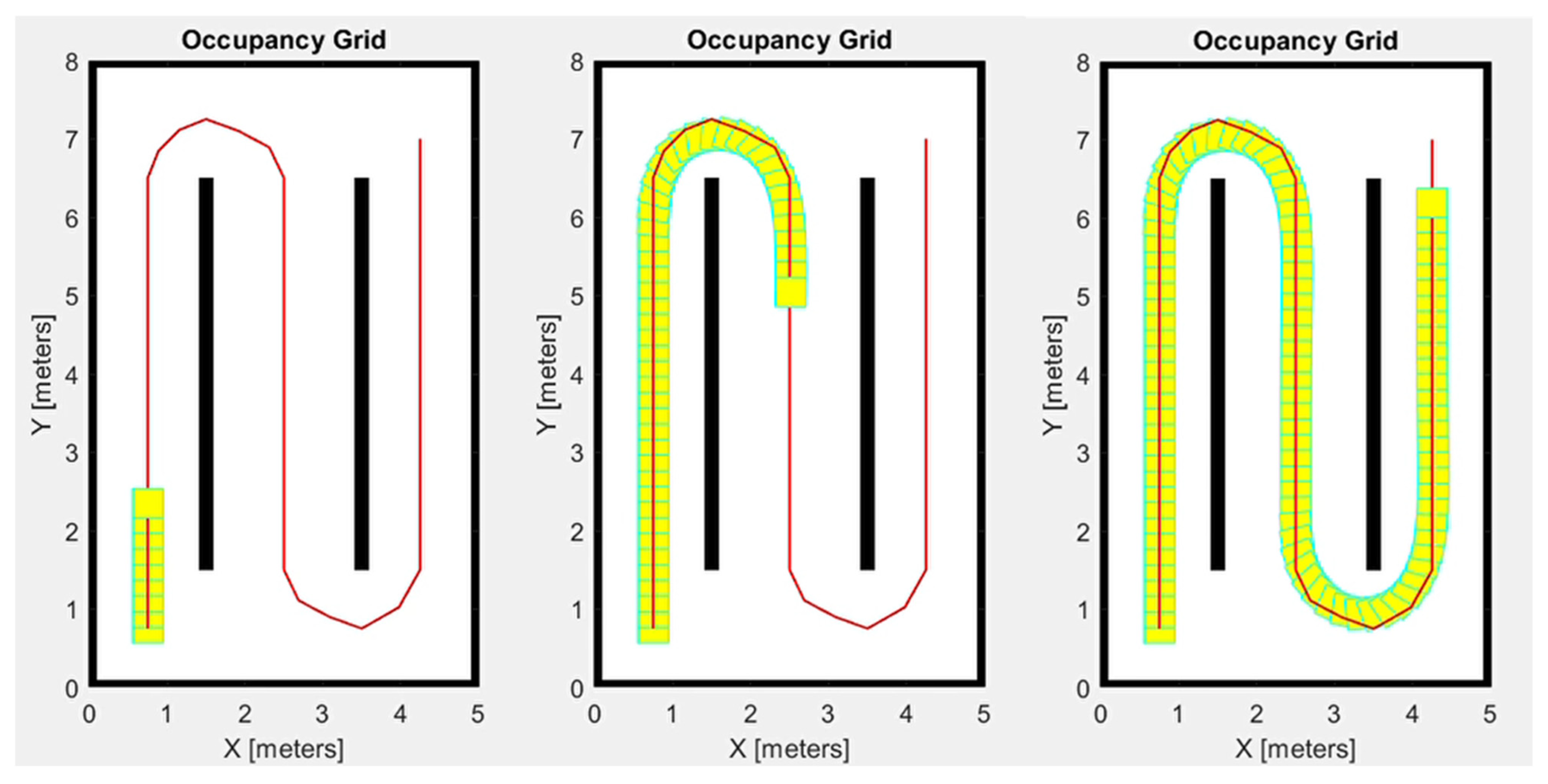
Figure 14.
In this figure, several frames from the start to the arrival point of the virtual simulation with the highest value of RA are shown; the highest value of RA occurs when LD and WPP are set to 1 m and 0.5 m, respectively, and this represents the best pursuit of the planned trajectory executed by the rover.
Once the best combination was identified, the accuracy error of the rover’s position was implemented to bring the simulations closer to the real-world case. The accuracy error consists of a random location error, added to the rover’s current position, before the calculation of the steering direction. The accuracy error varies at every time cycle and can range from 0 to the maximum settable accuracy error.
For this study, a maximum accuracy error of 2 cm was implemented, which is the maximum admissible accuracy value for a GPS-RTK positioning system [45,46,47], thus placing it in a worst-case condition. Furthermore, to improve the performance of the rover, a threshold value of 2.5° on the possible minimum steering angle was implemented. In this way, it is possible to avoid steering micro-corrections, which decrease the RA value without an actual decline in the vehicle performance. In Table 2, the results of three cases, the ideal one, the one with the accuracy error, and the one with the accuracy error and the steering angle threshold, are displayed.
Table 2.
Virtual model simulation results.
The third case represents the reference case, and it will be compared with the results obtained by the experimental field test.
3.2. Field Test Reuslts
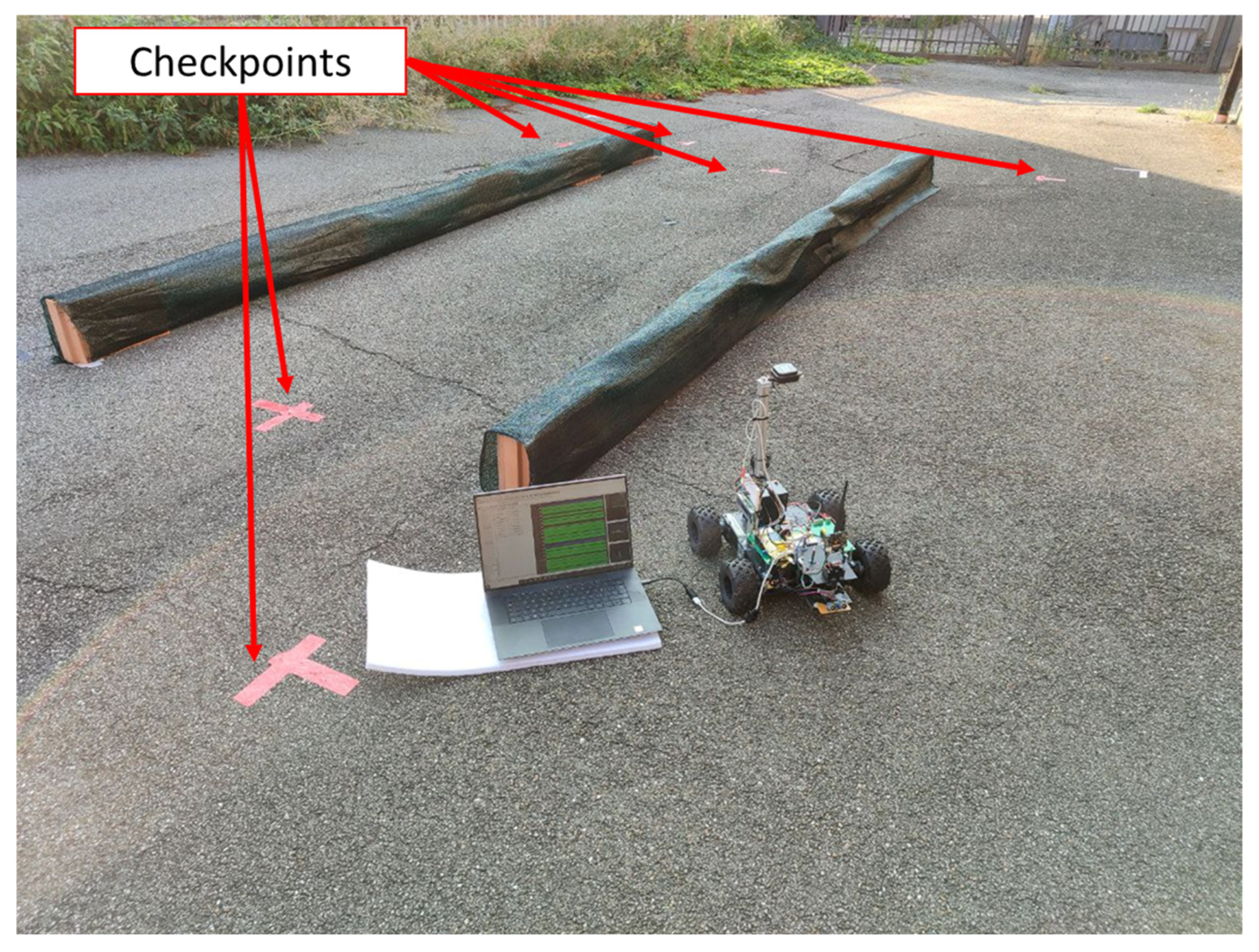
The field tests were performed according to the input parameters defined in Table 1 on the field visible in Figure 9. The first step of the field tests consists of the acquisition of the eight checkpoints (Figure 15).

Figure 15.
Checkpoint acquisition phase; red crosses marked on the road with adhesive tape represent the checkpoints defined for the execution of the field test.
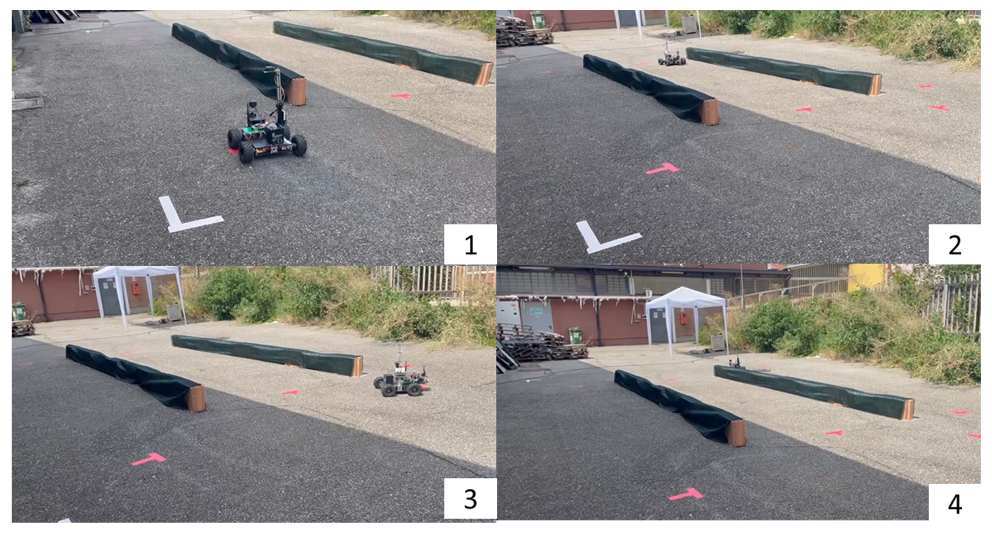
Then, the checkpoints and the values of LD and WPP, determined by the virtual model, were implemented in the algorithm. Hence, the field tests could be carried out correctly. Three field tests (Figure 16) were run to compare the experimental performance with the modeled tests. The parameters used for the field tests were the ones shown in Table 1 and they were the same as those used for the virtual analyses (WPP was set to 0.5 m and LD was set to 1 m) in order to compare them under the same conditions.
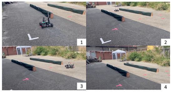
Figure 16.
Consecutive frames of one field test.
It must be noted that the algorithm works with a cartesian coordinate system, whereas the positioning system provides the rover’s position in terms of geodetic coordinates (latitude and longitude). Hence, the algorithm converts the geographical coordinates according to the following equation:
where
- X and Y are the projections of the geodetic coordinates in a cartesian reference system.
- Latitude and longitude are the geodetic coordinates provided by the positioning system.
- rearth is the mean value of the Earth’s radius and is equal to 6.371 × 10⁶ m.
Equations (6) and (7) are the projections of a sphere on a cartesian plane. This approximation of the geoid shape with a sphere surface can be considered valid when the considered surface is quite small like in this study. The trajectory of the three field tests obtained and referred to a cartesian coordinate system are shown in Figure 17.
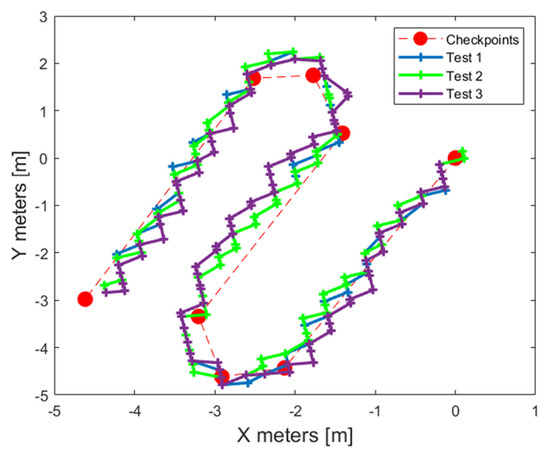
Figure 17.
Field test trajectories referred to the cartesian coordinate system.
The comparison between the field tests and the reference virtual case was made by evaluating the average trajectory deviations ATDs of each performance. Indeed, for real cases, it is quite impossible to evaluate the oscillating factor OF. In particular, during the simulation phase, the actual current position is always known, and the accuracy of the locating error operates only to determine the steering direction of the vehicle. Instead, during the real tests the current position of the vehicles is also affected by an accuracy error provided by the positioning system. The results of the field tests are shown in Table 3.
Table 3.
Field test results and comparison with the reference case.
The obtained results highlight that, in the majority of the performances carried out, the trajectory deviation is neglectable with respect to the virtual reference case. Actually, during Test 1, the performance was better than the virtual one. On average, the ATD percentage variation is around 10%. Speaking in absolute terms, the difference between the ATD of the real cases and the modeled one is just above 1 cm. Hence, the importance of the developed virtual model and its applicability in terms of developing the control logic for this kind of vehicle and applications emerged from the field tests campaign.
4. Conclusions
In this study, an autonomous driving strategy for an agricultural rover, equipped with a four-wheel differential drive system and operating in a vineyard/orchard environment was proposed. Then, a scale prototype was designed and assembled in order to verify the reliability of the developed autonomous driving algorithm. In this way, the virtual model developed could represent a powerful tool for the development of control logic for this kind of vehicle and these kinds of operative environments. The autonomous driving strategy is structured into two main parts: path planning and path following. The first step consists of the definition of the ideal trajectory that allows the rover to accomplish its mission. The second one allows the vehicle to follow the ideal trajectory in order to reach its specific goals. Two fundamental parameters must be tuned in order to enable the vehicle to follow the ideal trajectory properly, namely the look-ahead distance and the waypoint pitch distribution. Indeed, the aim of the virtual model is to find the best combination of these two parameters, on the basis of some performance indicators: average trajectory deviation, oscillating factor, and relative accuracy. Once the best combination was defined, an accuracy locating error and a minimum steering angle threshold were set. In this way, the behavior of the rover could be closer to the real case. At this point, a scale prototype was designed and assembled, and a vineyard/orchard replica was built in order to carry out some field tests and verify the applicability and reliability of the described motion strategy. From the campaign, it emerged that, in the majority of the performed tests, the differences with respect to the reference case were neglectable. So, the validity of the virtual model proposed can be considered verified and reliable. However, the results obtained from this study can be viewed as a starting point for further analysis and development. In particular, the virtual model can be improved especially during the execution of corners in order to reach higher values of relative accuracy. Another further improvement of the proposed strategy is the implementation of an obstacle avoidance strategy in order to avoid unexpected obstacles. In the end, the design of a 1:1 scale prototype is also necessary, so that several tests can be performed in a real vineyard/orchard environment.
Author Contributions
Conceptualization, S.M. and F.M.; methodology, S.M. and F.M.; software, S.M.; validation, S.M. and F.M.; formal analysis, S.M.; investigation, S.M.; data curation, S.M.; writing—original draft preparation, S.M.; writing—review and editing, S.M. and F.M.; visualization, S.M.; supervision, S.M and F.M. All authors have read and agreed to the published version of the manuscript.
Funding
This research received no external funding.
Institutional Review Board Statement
Not applicable.
Informed Consent Statement
Informed consent was obtained from all subjects involved in the study.
Data Availability Statement
The original contributions presented in this study are included in the article. Further inquiries can be directed to the corresponding author(s).
Conflicts of Interest
The authors declare no conflicts of interest.
References
- Martelli, S.; Mocera, F.; Somà, A. Carbon Footprint of an Orchard Tractor through a Life-Cycle Assessment Approach. Agriculture 2023, 13, 1210. [Google Scholar] [CrossRef]
- Praveen, B.; Sharma, P. A Review of Literature on Climate Change and Its Impacts on Agriculture Productivity. J. Public Aff. 2019, 19. [Google Scholar] [CrossRef]
- Wollenberg, E.; Richards, M.; Smith, P.; Havlík, P.; Obersteiner, M.; Tubiello, F.N.; Herold, M.; Gerber, P.; Carter, S.; Reisinger, A.; et al. Reducing Emissions from Agriculture to Meet the 2 °C Target. Glob. Change Biol. 2016, 22, 3859–3864. [Google Scholar] [CrossRef]
- Patz, J.A.; Campbell-Lendrum, D.; Holloway, T.; Foley, J.A. Impact of Regional Climate Change on Human Health. Nature 2005, 438, 310–317. [Google Scholar] [CrossRef]
- Stott, P. How Climate Change Affects Extreme Weather Events. Science 2016, 352, 1517–1518. [Google Scholar] [CrossRef]
- Christiaensen, L.; Rutledge, Z.; Taylor, J.E. Viewpoint: The Future of Work in Agri-Food. Food Policy 2021, 99, 101963. [Google Scholar] [CrossRef]
- Cirera, X.; Masset, E. Income Distribution Trends and Future Food Demand. Philos. Trans. R. Soc. B Biol. Sci. 2010, 365, 2821–2834. [Google Scholar] [CrossRef]
- Gohara-Beirigo, A.K.; Matsudo, M.C.; Cezare-Gomes, E.A.; de Carvalho, J.C.M.; Danesi, E.D.G. Microalgae Trends toward Functional Staple Food Incorporation: Sustainable Alternative for Human Health Improvement. Trends Food Sci. Technol. 2022, 125, 185–199. [Google Scholar] [CrossRef]
- Martelli, S.; Martini, V.; Mocera, F.; Soma’, A. Life Cycle Assessment Comparison of Orchard Tractors Powered by Diesel and Hydrogen Fuel Cell. Energies 2024, 17, 4599. [Google Scholar] [CrossRef]
- Bacenetti, J.; Lovarelli, D.; Facchinetti, D.; Pessina, D. An Environmental Comparison of Techniques to Reduce Pollutants Emissions Related to Agricultural Tractors. Biosyst. Eng. 2018, 171, 30–40. [Google Scholar] [CrossRef]
- Radrizzani, S.; Panzani, G.; Trezza, L.; Pizzocaro, S.; Savaresi, S.M. An Add-On Model Predictive Control Strategy for the Energy Management of Hybrid Electric Tractors. IEEE Trans. Veh. Technol. 2024, 73, 1918–1930. [Google Scholar] [CrossRef]
- Wang, S.; Wu, X.; Zhao, X.; Wang, S.; Xie, B.; Song, Z.; Wang, D. Co-Optimization Energy Management Strategy for a Novel Dual-Motor Drive System of Electric Tractor Considering Efficiency and Stability. Energy 2023, 281, 128074. [Google Scholar] [CrossRef]
- Gade, C.R.; Wahab, R.S. Conceptual Framework for Modelling of an Electric Tractor and Its Performance Analysis Using a Permanent Magnet Synchronous Motor. Sustainability 2023, 15, 14391. [Google Scholar] [CrossRef]
- Martini, V.; Mocera, F.; Somà, A. Carbon Footprint Enhancement of an Agricultural Telehandler through the Application of a Fuel Cell Powertrain. World Electr. Veh. J. 2024, 15, 91. [Google Scholar] [CrossRef]
- Jeon, H.-H.; Baek, S.-Y.; Baek, S.-M.; Choi, J.-Y.; Kim, Y.-S.; Kim, W.-S.; Kim, Y.-J. Efficiency Analysis of Powertrain for Internal Combustion Engine and Hydrogen Fuel Cell Tractor According to Agricultural Operations. Sensors 2024, 24, 5494. [Google Scholar] [CrossRef]
- Sharma, K.; Shivandu, S.K. Integrating Artificial Intelligence and Internet of Things (IoT) for Enhanced Crop Monitoring and Management in Precision Agriculture. Sens. Int. 2024, 5, 100292. [Google Scholar] [CrossRef]
- Mahore, V.; Patidar, P.; Soni, P.; Nagar, H.; Chouriya, A.; Paul, A. An IoT-Enabled Tractor Data Sensing System for Precision Agriculture. In Proceedings of the 2023 2nd International Conference on Futuristic Technologies (INCOFT), Belagavi, India, 24–26 November 2023; IEEE: Piscataway, NJ, USA, 2023; pp. 1–4. [Google Scholar]
- Roshanianfard, A.; Noguchi, N.; Okamoto, H.; Ishii, K. A Review of Autonomous Agricultural Vehicles (The Experience of Hokkaido University). J. Terramech. 2020, 91, 155–183. [Google Scholar] [CrossRef]
- Cheng, C.; Fu, J.; Su, H.; Ren, L. Recent Advancements in Agriculture Robots: Benefits and Challenges. Machines 2023, 11, 48. [Google Scholar] [CrossRef]
- Thakur, A.; Venu, S.; Gurusamy, M. An Extensive Review on Agricultural Robots with a Focus on Their Perception Systems. Comput. Electron. Agric. 2023, 212, 108146. [Google Scholar] [CrossRef]
- Sparrow, R.; Howard, M. Robots in Agriculture: Prospects, Impacts, Ethics, and Policy. Precis. Agric. 2021, 22, 818–833. [Google Scholar] [CrossRef]
- Archila, J.F.; Moreira, J.M.; Van Halts, V.I.; Alves, L.A.N.; Rueda, O.E.; Becker, M. Simulation of Rovers for Precision Agriculture. In Proceedings of the 2014 Joint Conference on Robotics: SBR-LARS Robotics Symposium and Robocontrol, Sao Carlos, Brazil, 18–23 October 2014; IEEE: Piscataway, NJ, USA, 2014; pp. 229–234. [Google Scholar]
- Crocetti, F.; Bellocchio, E.; Dionigi, A.; Felicioni, S.; Costante, G.; Fravolini, M.L.; Valigi, P. ARD-VO: Agricultural Robot Data Set of Vineyards and Olive Groves. J. Field Robot. 2023, 40, 1678–1696. [Google Scholar] [CrossRef]
- Wakchaure, M.; Patle, B.K.; Mahindrakar, A.K. Application of AI Techniques and Robotics in Agriculture: A Review. Artif. Intell. Life Sci. 2023, 3, 100057. [Google Scholar] [CrossRef]
- Mail, M.F.; Maja, J.M.; Marshall, M.; Cutulle, M.; Miller, G.; Barnes, E. Agricultural Harvesting Robot Concept Design and System Components: A Review. AgriEngineering 2023, 5, 777–800. [Google Scholar] [CrossRef]
- Ghafar, A.S.A.; Hajjaj, S.S.H.; Gsangaya, K.R.; Sultan, M.T.H.; Mail, M.F.; Hua, L.S. Design and Development of a Robot for Spraying Fertilizers and Pesticides for Agriculture. Mater Today Proc. 2023, 81, 242–248. [Google Scholar] [CrossRef]
- Lochan, K.; Khan, A.; Elsayed, I.; Suthar, B.; Seneviratne, L.; Hussain, I. Advancements in Precision Spraying of Agricultural Robots: A Comprehensive Review. IEEE Access 2024, 12, 129447–129483. [Google Scholar] [CrossRef]
- Li, S.; Xu, H.; Ji, Y.; Cao, R.; Zhang, M.; Li, H. Development of a Following Agricultural Machinery Automatic Navigation System. Comput. Electron. Agric. 2019, 158, 335–344. [Google Scholar] [CrossRef]
- Juman, M.A.; Wong, Y.W.; Rajkumar, R.K.; H’ng, C.Y. An Integrated Path Planning System for a Robot Designed for Oil Palm Plantations. In Proceedings of the TENCON 2017—2017 IEEE Region 10 Conference, Penang, Malaysia, 5–8 November 2017; IEEE: Piscataway, NJ, USA, 2017; pp. 1048–1053. [Google Scholar]
- Bai, Y.; Zhang, B.; Xu, N.; Zhou, J.; Shi, J.; Diao, Z. Vision-Based Navigation and Guidance for Agricultural Autonomous Vehicles and Robots: A Review. Comput. Electron. Agric. 2023, 205, 107584. [Google Scholar] [CrossRef]
- Martelli, S.; Mocera, F.; Somà, A. Co-Simulation of a Specialized Tractor for Autonomous Driving in Orchards; SAE International: Warrendale, PA, USA, 2022. [Google Scholar]
- Bayar, G.; Bergerman, M.; Koku, A.B.; Konukseven, E. ilhan Localization and Control of an Autonomous Orchard Vehicle. Comput. Electron. Agric. 2015, 115, 118–128. [Google Scholar] [CrossRef]
- Wang, H.; Noguchi, N. Autonomous Maneuvers of a Robotic Tractor for Farming. In Proceedings of the 2016 IEEE/SICE International Symposium on System Integration (SII), Sapporo, Japan, 13–15 December 2016; IEEE: Piscataway, NJ, USA, 2016; pp. 592–597. [Google Scholar]
- Peng, C.; Wei, P.; Fei, Z.; Zhu, Y.; Vougioukas, S.G. Optimization-based Motion Planning for Autonomous Agricultural Vehicles Turning in Constrained Headlands. J. Field Robot. 2024, 41, 1984–2008. [Google Scholar] [CrossRef]
- Han, X.; Lai, Y.; Wu, H. A Path Optimization Algorithm for Multiple Unmanned Tractors in Peach Orchard Management. Agronomy 2022, 12, 856. [Google Scholar] [CrossRef]
- Lujak, M.; Sklar, E.; Semet, F. Agriculture Fleet Vehicle Routing: A Decentralised and Dynamic Problem. AI Commun. 2021, 34, 55–71. [Google Scholar] [CrossRef]
- Gonzalez-de-Soto, M.; Emmi, L.; Gonzalez-de-Santos, P. Hybrid-Powered Autonomous Robots for Reducing Both Fuel Consumption and Pollution in Precision Agriculture Tasks. In Agricultural Robots-Fundamentals and Applications; IntechOpen: London, UK, 2019. [Google Scholar]
- Santos, L.; Santos, F.; Mendes, J.; Costa, P.; Lima, J.; Reis, R.; Shinde, P. Path Planning Aware of Robot’s Center of Mass for Steep Slope Vineyards. Robotica 2020, 38, 684–698. [Google Scholar] [CrossRef]
- Conesa-Muñoz, J.; Gonzalez-de-Soto, M.; Gonzalez-de-Santos, P.; Ribeiro, A. Distributed Multi-Level Supervision to Effectively Monitor the Operations of a Fleet of Autonomous Vehicles in Agricultural Tasks. Sensors 2015, 15, 5402–5428. [Google Scholar] [CrossRef]
- Martelli, S.; Mocera, F.; Somà, A. Autonomous Driving Strategy for a Specialized Four-Wheel Differential-Drive Agricultural Rover. AgriEngineering 2024, 6, 1937–1958. [Google Scholar] [CrossRef]
- Dubins, L.E. On Curves of Minimal Length with a Constraint on Average Curvature, and with Prescribed Initial and Terminal Positions and Tangents. Am. J. Math. 1957, 79, 497. [Google Scholar] [CrossRef]
- Hameed, I.A. Coverage Path Planning Software for Autonomous Robotic Lawn Mower Using Dubins’ Curve. In Proceedings of the 2017 IEEE International Conference on Real-time Computing and Robotics (RCAR), Okinawa, Japan, 14–18 July 2017; IEEE: Piscataway, NJ, USA, 2017; pp. 517–522. [Google Scholar]
- Macenski, S.; Singh, S.; Martín, F.; Ginés, J. Regulated Pure Pursuit for Robot Path Tracking. Auton. Robot. 2023, 47, 685–694. [Google Scholar] [CrossRef]
- Cornejo, J.; Magallanes, J.; Denegri, E.; Canahuire, R. Trajectory Tracking Control of a Differential Wheeled Mobile Robot: A Polar Coordinates Control and LQR Comparison. In Proceedings of the 2018 IEEE XXV International Conference on Electronics, Electrical Engineering and Computing (INTERCON), Lima, Peru, 8–10 August 2018; IEEE: Piscataway, NJ, USA, 2018; pp. 1–4. [Google Scholar]
- Ekaso, D.; Nex, F.; Kerle, N. Accuracy Assessment of Real-Time Kinematics (RTK) Measurements on Unmanned Aerial Vehicles (UAV) for Direct Geo-Referencing. Geo-Spat. Inf. Sci. 2020, 23, 165–181. [Google Scholar] [CrossRef]
- Baertlein, H.; Carlson, B.; Eckels, R.; Lyle, S.; Wilson, S. A High-Performance, High-Accuracy RTK GPS Machine Guiadance System. GPS Solut. 2000, 3, 4–11. [Google Scholar] [CrossRef]
- Pirti, A. Evaluating the Repeatability of RTK GPS. Surv. Rev. 2011, 43, 177–186. [Google Scholar] [CrossRef]


Disclaimer/Publisher’s Note: The statements, opinions and data contained in all publications are solely those of the individual author(s) and contributor(s) and not of MDPI and/or the editor(s). MDPI and/or the editor(s) disclaim responsibility for any injury to people or property resulting from any ideas, methods, instructions or products referred to in the content. |
© 2025 by the authors. Licensee MDPI, Basel, Switzerland. This article is an open access article distributed under the terms and conditions of the Creative Commons Attribution (CC BY) license (https://creativecommons.org/licenses/by/4.0/).