A Combined Approach of Experimental Testing and Inverse FE Modelling for Determining Homogenized Elastic Properties of Membranes and Plates ^†

Abstract

Accurately determining the mechanical properties of complex materials is a key challenge in structural analysis, especially when using the finite element method (FEM). While homogeneous materials can be modeled with relative ease, heterogeneous materials such as composites or biological tissues with multiphase compositions pose significant difficulties due to the variability in their internal structures. The most used approach is numerical homogenization, which allows for the estimation of effective material properties by combining the characteristics of individual phases; however, this technique may not always be feasible, especially for materials with irregular or unknown phase distributions. This paper proposes an original methodology that combines non-destructive experimental testing with an inverse finite element modeling to extract the anisotropic elastic properties of quasi two-dimensional structures such as membranes and plates. The method involves modeling the component using membrane or plate finite elements, but managing a global stiffness matrix expressed analytically. While geometric information is incorporated in the global stiffness matrix, the material properties, specifically the components of the anisotropic elasticity matrix, remain unknown. The experimental data, comprising force and displacement measurements, are used to solve a nonlinear system, allowing for the identification of the material’s constitutive properties via numerical computation. To validate this approach, two experimental setups were conducted. The first involved a hyperelastic neoprene membrane, subjected to various biaxial preloading conditions, while the second focused on PLA plates produced through additive manufacturing including both homogeneous and reinforced variants. In both cases, the method successfully captured the full anisotropic elastic response, yielding accurate estimates of Young’s moduli, Poisson’s ratios, shear modulus, and orthotropy system orientation, in agreement with independent mechanical tests. This combined approach offers a practical and efficient solution for determining the elastic properties of complex materials, particularly in cases where traditional homogenization techniques are impractical or inadequate. Furthermore, this method can be a versatile tool for evaluating the damaging and aging effects on materials subjected to cyclic loading or those with irregular and complex internal structures.

1. Introduction

In structural analysis, commonly performed through the finite element method (FEM), the precise knowledge of mechanical properties of complex materials, especially those with a multiphase composition, is an important issue. The mechanical performance of a material directly influences the reliability and accuracy of structural simulations, which are essential for designing safe and efficient engineering systems. For structures made from homogeneous materials, creating a CAD model and dividing it into subregions for the subsequent FE analysis is often straightforward and sufficient [1,2]. However, the process becomes more challenging when dealing with heterogeneous materials such as composites or biological materials with varying internal phases. In such cases, an unknown or irregular composition can lead to significant difficulties in modeling and simulation.

The principal trouble in these situations lies in accurately defining the mechanical properties and geometry of each phase present within the material or structure. For instance, in multi-material tubes, composite plates, or membranes composed of biological tissues, granular or porous materials, each phase may exhibit distinct mechanical behaviors [1,3]. These behaviors could include variations in stiffness, strength, or anisotropy that are dependent on the material’s internal structure. The challenge, therefore, is to either fully characterize each phase mechanically and geometrically or, at a minimum, to determine an overall mechanical response that represents a homogenized or averaged behavior of the entire material.

One effective approach to address this complexity is through the application of homogenization techniques [4,5,6,7]. Homogenization is a method that allows for the derivation of the effective mechanical properties of a composite or multiphase material by combining the properties of its individual constituents and considering their spatial arrangement. The result is a set of averaged or “homogenized” properties that can be used in structural analysis as a substitute for detailed phase-specific information. This approach is particularly useful in engineering applications where modeling the full complexity of the material on a phase-by-phase basis would be computationally prohibitive or impractical.

Homogenization techniques typically rely on the construction of a representative volume element (RVE) [8], a small but sufficiently detailed model of the material that captures its essential characteristics. The RVE is used to simulate the mechanical response of the material under various loading conditions. By analyzing the behavior of this element, it is possible to derive an effective elastic constitutive matrix that represents the homogenized mechanical properties of the material. These properties include stiffness and anisotropic behavior, which are essential for predicting how the material performs in engineering applications. The accuracy of this homogenization process depends on several factors including the size of the RVE, the orientation and geometry of the individual phases, and the level of discretization used in the model.

The success of this approach has led to its widespread adoption in many fields of engineering, particularly for materials with complex microstructures such as fiber-reinforced composites, porous materials, and cellular structures. In these materials, the mechanical properties can vary significantly at the microscopic level, but homogenization allows one to obtain a macroscopic description suitable for structural design and analysis.

Despite its widespread use, numerical homogenization is not always feasible or applicable. There are certain classes of materials for which the standard homogenization techniques may encounter significant difficulties. These materials often exhibit complex internal phase distributions that cannot be easily captured by traditional modeling approaches. For example, materials with a pseudo-random distribution of phases, such as composites with medium to short fibers or biological tissues with irregular structures, pose a significant challenge [9,10]. In these cases, the geometric arrangement of the phases, their volumetric fractions, and their individual mechanical behaviors may not be fully known or may be too complex to model accurately.

Other examples where numerical homogenization may fail include structurally damaged materials such as reinforced concrete elements or composite plates subjected to cyclic loading or aging, where the material’s microstructure has been altered in unpredictable ways [11,12]. Another important case concerns biological materials, where the internal phase distribution may not only be random, but also vary between samples due to natural biological variation. Additionally, mechanical components that require a multiphysics approach, such as hollow pipes filled with internal gas and subjected to bending, present other layers of complexity; in these cases, the interaction between different physical phenomena cannot be adequately captured through numerical homogenization techniques.

For materials with such complex internal structures, the homogenized anisotropic elastic response may only be obtainable through direct experimental testing. By subjecting the mechanical component or material to controlled loading and boundary conditions, it is possible to measure the material’s overall response and derive its effective mechanical properties empirically. The experimental information encompasses all the complexity of the material, offering a more accurate means of determining the effective mechanical properties when numerical approaches fall short or prove inadequate.

To address this issue, Iandiorio and Salvini [13] proposed a combined approach of experimental testing and inverse FE modeling based on flexibility to obtain the elastic constitutive properties of composite beam elements.

In order to extend the idea to higher order type of elements and geometries, this paper discusses a method through which it is possible to determine the homogenized elastic anisotropic constitutive matrix of quasi two-dimensional elements, such as membranes and plates, using a combined approach of experimental testing and inverse finite element (FE) modeling. The required experimental stiffness measurements are simple and of the non-destructive type, making this method particularly useful for assessing the damage state of materials subjected to cyclic loading. In other words, the proposed approach offers a practical solution for evaluating complex materials where conventional methods may be insufficient and can be applied without compromising the integrity of the material.

2. The Idea to Combine Experimental Tests and an Inverse Finite Element Analysis and How to Implement It

Iandiorio and Salvini in [13] proposed a method to obtain the anisotropic elastic constitutive properties of rectilinear beam elements. The method exposed in [13] involves conducting flexibility measurements, which are simpler than stiffness tests for beam elements, and then processing the results through inverse flexibility-based finite element modeling [14,15] to build-up the stiffness matrix of the element. By employing the relationship between the complementary energy and flexibility, [13] showed how to extract the components that define the constitutive matrix of the material, containing information on the material, geometry, and inertia of the beams’ cross-section for the beam elements.

Before developing the procedure presented in this paper, we attempted to extend the flexibility-based finite element modeling approach from [13] to membrane and plate elements. However, this approach was not pursued due to the significant challenges associated with using a flexibility-based method for higher-order elements. We believe it is beneficial for the reader to summarize these difficulties. The flexibility-based finite element method has been a leading approach in engineering for nearly three decades, on par with stiffness-based methods [16,17]. Its appeal, especially at a time when computational power was much more limited than in recent decades, lies in the fact that it handles smaller systems of equations and, in cases where only the displacements at the free degrees of freedom are of interest, it does not require matrix inversion. However, its decline compared with stiffness-based approaches stems from difficulties in managing the redundant constraint forces [18] of large structures and formulating stress-based shape functions for 2D and 3D elements. For planar elements, stress-based shape functions are derived from integrating the Beltrami–Mitchell equations [19]. As is well-known, this can only be carried out analytically and leads to the exact form only in specific cases. For a finite element with a generic number of nodes, one must settle for a truncated power series expansion of the stress potential function (Airy’s function). Furthermore, the core issue is that the Beltrami–Mitchell equations are material-independent only in the case of isotropic materials. For materials with generic anisotropy, as in the case addressed in this paper, the shape functions derived using this approach would already depend on the components of the elastic matrix of the material, which is not the case for stiffness-based elements. These complications, along with the fact that most commercial codes are stiffness-based, led the authors to abandon the flexibility approach in favor of a stiffness-based formulation.

In what follows, this section outlines the idea and the procedure for combining simple experimental tests with an inverse FE modeling approach, based on stiffness, to determine the homogenized elastic matrix of the material within a quasi-two-dimensional mechanical component.

As is well-known, the fundamental equation that governs the statics of the linear deformable structure discretized according the stiffness-based FE modeling is [20]:

$$\left[\mathit{K}\right]\left\{\mathit{U}\right\}=\left\{\mathit{F}\right\}$$

(1)

where $\left\{\mathit{U}\right\}$ is the displacements vector, $\left\{\mathit{F}\right\}$ is the forces vector, and $\left[\mathit{K}\right]$ is the global stiffness matrix that is derived from the assembling procedure of all the stiffness matrices of the elements. The stiffness matrix of a single element is defined as:

$$\left[{\mathit{K}}^{el}\right]=\underset{V}{\int }{\left[\mathit{B}\right]}^T\left[\mathit{D}\right]\left[\mathit{B}\right]dV$$

(2)

where $\left[\mathit{B}\right]$ is the matrix that gives the deformation vector of the elements knowing the nodal displacements vector of the element itself; $V$ is the element’s volume; $\left[\mathit{D}\right]$ is the symmetric elastic constitutive matrix of the material forming the element. It depends, in its general anisotropic form and for two-dimensional elements, on six elastic constants $d_{ij}$:

$$\left[\mathit{D}\right]=\left[\begin{array}{ccc}{d}_{11}& d_{12}& d_{13}\\ & d_{22}& d_{23}\\ Sym& & d_{33}\end{array}\right]$$

(3)

The key point is that the presented method deals with an unknown material and aims to determine the six elastic constants that define $\left[\mathit{D}\right]$. To achieve this, one can analytically integrate Equation (2), incorporating only the geometric information of the element after the integration, while leaving the six material constants as unknown variables. This is complex to perform by hand calculations but is quite straightforward using symbolic algebra software. Clearly, transitioning to a fully analytical expression of Equation (2) has limitations regarding the types of elements that can be used. Specifically, it is not possible to analytically integrate Equation (2) for isoparametric elements [20], which are known to involve a complex expression of the Jacobian matrix determinant during the transformation to natural coordinates. However, this can be conducted for non-isoparametric elements such as membrane elements [21] and plates defined in the physical reference system [22]. If this is carried out, Equation (1) becomes:

$$\left[\mathit{K}\left(d_{ij}\right)\right]\left\{\mathit{U}\right\}=\left\{\mathit{F}\right\}$$

(4)

where $\left[\mathit{K}\left(d_{ij}\right)\right]$ is the assembled global stiffness matrix of the structure, that is function of the six material constants $d_{ij}$.

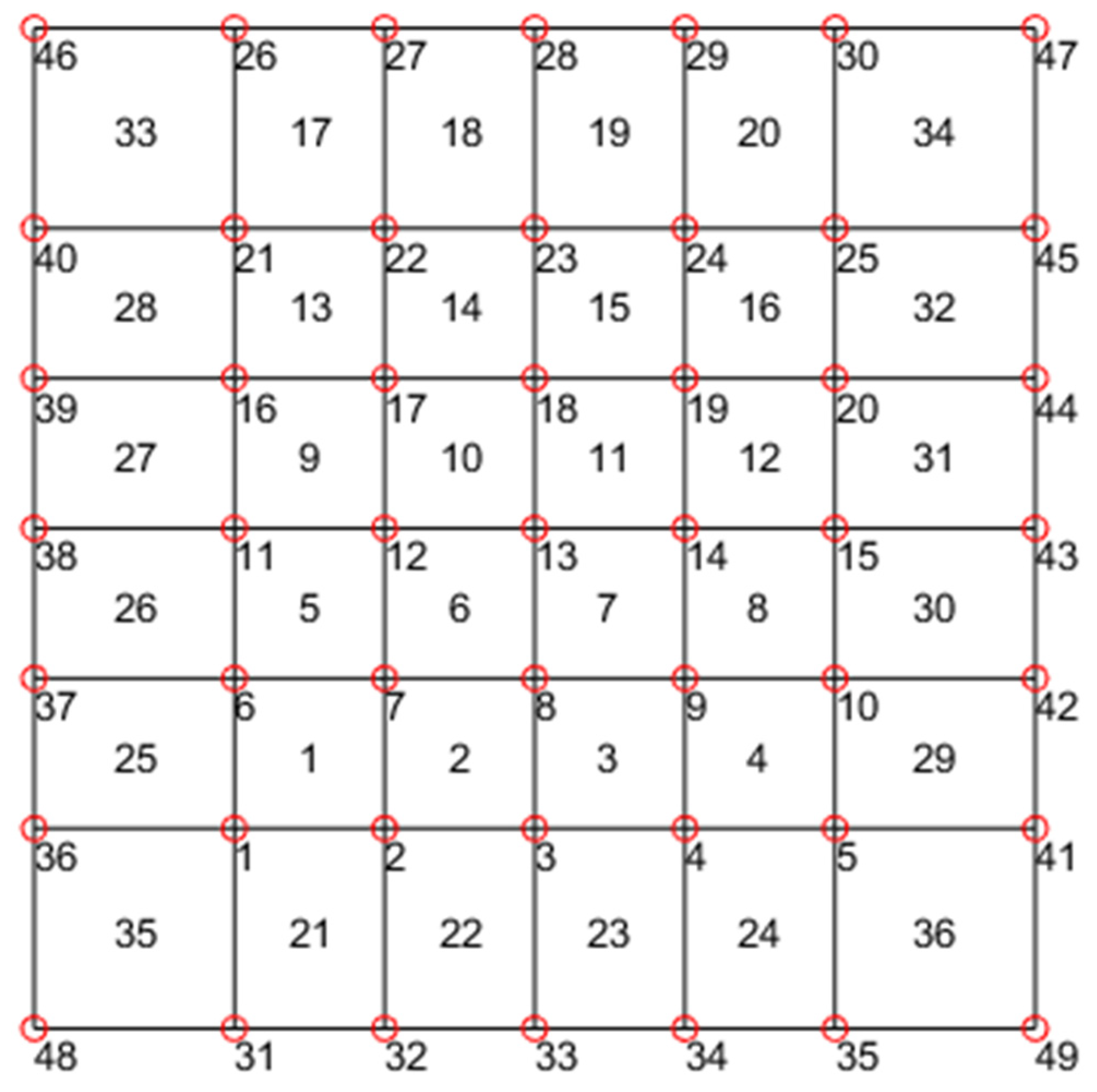
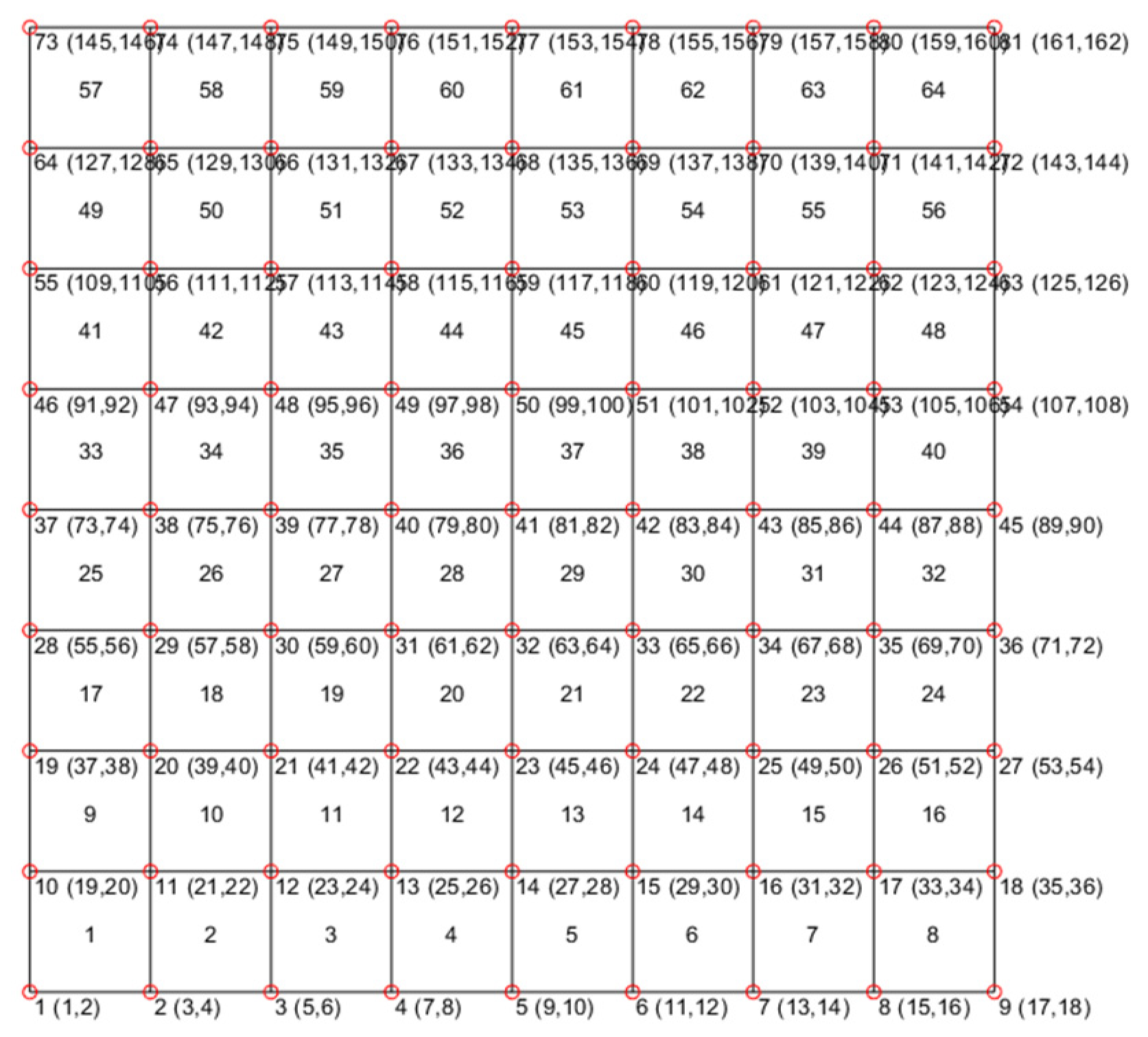
Equation (4) should be interpreted differently from Equation (1), as now the idea is that some components of the vectors $\left\{\mathit{U}\right\}$ and $\left\{\mathit{F}\right\}$ are already known from the experimental tests. To better understand this step, refer to the example in Figure 1, which shows a plate clamped at the edges and loaded at its center perpendicularly to its plane. If this plate is discretized using plate elements, a distinction must be made between the free and constrained degrees of freedom (DOFs). Therefore, the partitioned form of Equation (4) becomes:

$$\left[\begin{array}{cc}\left[{\mathit{K}}_{ff}\left(d_{ij}\right)\right]& \left[{\mathit{K}}_{fc}\left(d_{ij}\right)\right]\\ \left[{\mathit{K}}_{cf}\left(d_{ij}\right)\right]& \left[{\mathit{K}}_{cc}\left(d_{ij}\right)\right]\end{array}\right]\left\{\begin{array}{c}\left\{{\mathit{U}}_f\right\}\\ \left\{{\mathit{U}}_c\right\}\end{array}\right\}=\left\{\begin{array}{c}\left\{{\mathit{F}}_f\right\}\\ \left\{{\mathit{F}}_c\right\}\end{array}\right\}$$

(5)

where the subscripts “f” and “c” denote the free and constrained DOFs, respectively.

The displacements associated with the constrained degrees of freedom are zero, thus $\left\{{\mathit{U}}_c\right\}=\left\{\mathbf{0}\right\}$, while no assumptions can be made regarding the forces acting along those constrained DOFs. Regarding the displacements and forces on the free DOFs, it is useful to distinguish them into two subsets, referred to as master and slave: $\left\{{\mathit{U}}_f\right\}={\left\{\left\{{\mathit{U}}_{fm}\right\},\left\{{\mathit{U}}_{fs}\right\}\right\}}^T$ and $\left\{{\mathit{F}}_f\right\}={\left\{\left\{{\mathit{F}}_{fm}\right\},\left\{{\mathit{F}}_{fs}\right\}\right\}}^T$. The displacements and forces associated with the free master DOFs (i.e., $\left\{{\mathit{U}}_{fm}\right\},\left\{{\mathit{F}}_{fm}\right\}$) are those DOFs for which both the forces and displacements are known from the experimental data. These are the points where the load is applied (e.g., in Figure 1, the only master DOF is indicated in red). As a consequence, no external forces are applied at the free DOFs of slave type (i.e., $\left\{{\mathit{F}}_{fs}\right\}=\left\{\mathbf{0}\right\}$).

Equation (5) can therefore be partitioned as follows:

$$\left[\begin{array}{ccc}\left[{\mathit{K}}_{fmfm}\left(d_{ij}\right)\right]& \left[{\mathit{K}}_{fmfs}\left(d_{ij}\right)\right]& \left[{\mathit{K}}_{fmfc}\left(d_{ij}\right)\right]\\ \left[{\mathit{K}}_{fsfm}\left(d_{ij}\right)\right]& \left[{\mathit{K}}_{fsfs}\left(d_{ij}\right)\right]& \left[{\mathit{K}}_{fsc}\left(d_{ij}\right)\right]\\ \left[{\mathit{K}}_{cfm}\left(d_{ij}\right)\right]& \left[{\mathit{K}}_{cfs}\left(d_{ij}\right)\right]& \left[{\mathit{K}}_{cc}\left(d_{ij}\right)\right]\end{array}\right]\left\{\begin{array}{c}\left\{{\mathit{U}}_{fm}\right\}\\ \left\{{\mathit{U}}_{fs}\right\}\\ \left\{\mathbf{0}\right\}\end{array}\right\}=\left\{\begin{array}{c}\left\{{\mathit{F}}_{fm}\right\}\\ \left\{\mathbf{0}\right\}\\ \left\{{\mathit{F}}_c\right\}\end{array}\right\}$$

(6)

Considering only the free DOFs and applying the static condensation [22] to eliminate the slave DOFs, since the displacement vector $\left\{{\mathit{U}}_{fs}\right\}$ is unknown from experimental tests, the following expression is obtained:

$$\left[{\mathit{K}}_{cond}\left(d_{ij}\right)\right]\left\{{\mathit{U}}_{fm}\right\}=\left\{{\mathit{F}}_{fm}\right\}$$

(7)

where the condensed stiffness matrix is:

$$\left[{\mathit{K}}_{cond}\left(d_{ij}\right)\right]=\left(\left[{\mathit{K}}_{fmfm}\left(d_{ij}\right)\right]-\left[{\mathit{K}}_{fmfs}\left(d_{ij}\right)\right]{\left[{\mathit{K}}_{fsfs}\left(d_{ij}\right)\right]}^{-1}\left[{\mathit{K}}_{fsfm}\left(d_{ij}\right)\right]\right)$$

(8)

Generally, to gather sufficient information to reliably derive the elasticity matrix in Equation (3), it is necessary to apply the load individually at different points. In this case, to build-up the nonlinear system, Equation (8) must be written as many times as the number of load tests performed, resulting in:

$$\left\{\begin{array}{c}\left[{\mathit{K}}_{cond}^1\left(d_{ij}\right)\right]\left\{{\mathit{U}}_{fm}^1\right\}=\left\{{\mathit{F}}_{fm}^1\right\}\\ \left[{\mathit{K}}_{cond}^2\left(d_{ij}\right)\right]\left\{{\mathit{U}}_{fm}^2\right\}=\left\{{\mathit{F}}_{fm}^2\right\}\\ \begin{array}{c}⋮\\ \begin{array}{c}⋮\\ \left[{\mathit{K}}_{cond}^n\left(d_{ij}\right)\right]\left\{{\mathit{U}}_{fm}^n\right\}=\left\{{\mathit{F}}_{fm}^n\right\}\end{array}\end{array}\end{array}\right.$$

(9)

where $n$ is the number of loadings.

It is worth pointing out that for each load, the enumeration of master and slave DOFs taken into account on each row of Equation (9) changes.

Equation (9) can be visualized as a generic nonlinear system of equations, in other words,

$$\left\{\mathit{f}\left(d_{ij}\right)\right\}=\left\{\mathbf{0}\right\}$$

(10)

The solution to Equation (10) can only be obtained numerically. Even solving it through numerical techniques is not straightforward, as the solution must satisfy the constraint of positive definiteness of Equation (3). To address this issue, we chose to adopt a reliable technique recently used in [23,24,25] to solve a structural problem, similar to Equation (10), involving a thousand number of unknowns. It consists of solving Equation (10) by using the power of optimization algorithms, therefore transforming the problem of Equation (10) into:

$$\left\{\begin{array}{c}\min \Psi \left(d_{ij}\right)\\ \\ \mathrm{s}\mathrm{u}\mathrm{c}\mathrm{h}\mathrm{t}\mathrm{h}\mathrm{a}\mathrm{t}{d}_{11},d_{22},d_{33}>0\end{array}\right.$$

(11)

where:

$$\Psi \left(d_{ij}\right)=‖\left\{\mathit{f}\left(d_{ij}\right)\right\}‖$$

(12)

Due to the convexity of Equation (12), it becomes clear that if Equation (10) is fully satisfied, then Equation (12) reaches a condition of strong minimum.

One significant advantage of Equation (11) is its feature to offer insights into the nature of the solution. In most optimization algorithms, it is generally difficult to determine whether a solution corresponds to a weak or strong minimum. However, in this case, the residue produced when the solution of Equation (11) is substituted into Equation (10) can be evaluated. This unique feature enables the use of a straightforward and robust convergence criterion:

$${\displaystyle \frac{\Psi \left(d_{ij}\right)}{‖{\mathit{F}}_{fm}‖}}\le tol$$

(13)

where $tol$ is a tolerance value, and $‖\left\{{\mathit{F}}_{fm}\right\}‖=‖{\left\{\left\{{\mathit{F}}_{fm}^1\right\},\left\{{\mathit{F}}_{fm}^2\right\},\dots ,\left\{{\mathit{F}}_{fm}^n\right\}\right\}}^T‖$.

Another important aspect is the choice of a trial solution. In the following examples, a reliable starting solution was provided using an isotropic elasticity matrix, which requires only two material constants. Typically, the order of magnitude of these constants for the material being analyzed is known, offering a solid initial approximation.

3. Validation of the Procedure: Experimental Tests on Membranes and Plates

This section presents two experimental case studies, one for membranes and one for plates, where the procedure outlined in the previous section was applied.

3.1. Determination of the Anisotropic Elastic Properties of Membranes

To carry out experimental tests on the membranes, neoprene, commonly used in diving suits, was the chosen material due to its elastomeric properties. The material strips were cut from the front of the suit, which exhibited different textures and stitching patterns in two orthogonal directions, leading to variations in resistance along these axes. To assess these differences, tensile tests were conducted on two separate strips of material aligned with the aforementioned orientations. The results of these tests, as presented in Figure 2, revealed that both cases yielded an initial tangent modulus of 0.3 MPa. The latter value is useful for assessing the following outcomes concerning the determination of the membrane’s constitutive matrix.

The membrane sample was fitted with nine studs (see Figure 3a), in order to establish specific load application zones. This sample was then locked within a wooden frame designed to allow for the application of a pre-load on the membrane. The membrane was loaded using calibrated harmonic steel springs (Figure 4), which were applied between the central stud and one of the lateral studs for a total of eight applications. The loading sequences are illustrated in Figure 5.

Through digital image acquisition of the deformed configurations, we proceeded to collect the displacements on the loaded DOFs, which were used in Equation (9). The acting forces were determined from the displacements via the elastic constants of the springs shown in Figure 4. The membrane was modeled using four-node plane elements [21], and the mesh utilized in our custom software for data processing is represented in Figure 6. Given the simple geometry of the analyzed membrane, the mesh consisted of 64 geometrically identical elements, allowing for the analytical computation of the stiffness matrix.

The loading procedure was applied for various preload levels of the membrane. The preload was introduced by applying a strain of 15% or 30% relative to the initial length of the membrane’s side. Specifically, the test cases included 0–30%, 15–30%, and 30–30%, where the first number in the pair indicates the preload along the strong direction (red arrow in Figure 3a), and the second number indicates the preload along the weak direction (blue arrow in Figure 3a).

The results of the post-processing of the experimental tests, conducted in accordance with the procedure outlined in Section 2, are summarized in

Table 1. Results with a preload of 0% and 30% along the strong and weak directions, respectively.

Elastic Constants in the Experimental Reference System	Elastic Constants in the Orthotropy Reference System
	$\vartheta =-0.013\mathrm{d}\mathrm{e}\mathrm{g}$	$G_{1^{\prime }{2}^{\prime }}=0.007\mathrm{M}\mathrm{P}\mathrm{a}$
${\left[\mathit{D}\right]}_{0-30}={10}^5\left[\begin{array}{ccc}1.439& 4.315& 0.004\\ & 1.585& 0.003\\ Sym& & 0.070\end{array}\right]$	$E_{1^{\prime }}=0.115\mathrm{M}\mathrm{P}\mathrm{a}$	$E_{2^{\prime }}=0.127\mathrm{M}\mathrm{P}\mathrm{a}$
	${\nu }_{1^{\prime }{2}^{\prime }}=0.422$	${\nu }_{2^{\prime }{1}^{\prime }}=0.465$

,

Table 2. Results with a preload of 15% and 30% along the strong and weak directions, respectively.

Elastic Constants in the Experimental Reference System	Elastic Constants in the Orthotropy Reference System
	$\vartheta =31.13\mathrm{d}\mathrm{e}\mathrm{g}$	$G_{1^{\prime }{2}^{\prime }}=0.007\mathrm{M}\mathrm{P}\mathrm{a}$
${\left[\mathit{D}\right]}_{15-30}={10}^5\left[\begin{array}{ccc}1.860& 1.932& -0.253\\ & 2.494& -0.381\\ Sym& & 0.011\end{array}\right]$	$E_{1^{\prime }}=0.131\mathrm{M}\mathrm{P}\mathrm{a}$	$E_{2^{\prime }}=0.254\mathrm{M}\mathrm{P}\mathrm{a}$
	${\nu }_{1^{\prime }{2}^{\prime }}=0.248$	${\nu }_{2^{\prime }{1}^{\prime }}=0.486$

and

Table 3. Results with a preload of 30% and 30% along the strong and weak directions, respectively.

Elastic Constants in the Experimental Reference System	Elastic Constants in the Orthotropy Reference System
	$\vartheta =-17.56\mathrm{d}\mathrm{e}\mathrm{g}$	$G_{1^{\prime }{2}^{\prime }}=0.01\mathrm{M}\mathrm{P}\mathrm{a}$
${\left[\mathit{D}\right]}_{30-30}={10}^5\left[\begin{array}{ccc}4.043& 3.710& -0.048\\ & 3.124& -0.274\\ Sym& & 0.018\end{array}\right]$	$E_{1^{\prime }}=0.337\mathrm{M}\mathrm{P}\mathrm{a}$	$E_{2^{\prime }}=0.244\mathrm{M}\mathrm{P}\mathrm{a}$
	${\nu }_{1^{\prime }{2}^{\prime }}=0.486$	${\nu }_{2^{\prime }{1}^{\prime }}=0.352$

. On the left side of each table, the anisotropic elastic matrix resulting directly from the computation of Equation (11) is shown. This matrix already contains all the information regarding the homogenized elastic properties of the component, but can be further investigated. As is well-known from elasticity theory, the tensor $\left[\mathit{D}\right]$ expressed in the reference system $\left\{\mathrm{1,2}\right\}$ (Figure 3a) can be expressed in a rotated reference system $\left\{1^{\prime },2^{\prime }\right\}$ through the following change of basis [25]:

$$\left[{\mathit{D}}_{rot}\right]=\left[\mathit{T}\right]\left[\mathit{D}\right]{\left[\mathit{T}\right]}^T$$

(14)

where $\left[\mathit{T}\right]$ is the change in the basis matrix, expressed through the knowledge of the angle $\vartheta$, which is the angle that aligns the original reference system with the new reference system, measured counterclockwise:

$$\left[\mathit{T}\right]=⌈\begin{array}{ccc}{\cos }^2\vartheta & {\sin }^2\vartheta & -2\sin \vartheta \cos \vartheta \\ {\sin }^2\vartheta & {\cos }^2\vartheta & 2\sin \vartheta \cos \vartheta \\ \sin \vartheta \cos \vartheta & -\sin \vartheta \cos \vartheta & {\cos }^2\vartheta -{\sin }^2\vartheta \end{array}⌉$$

(15)

Using Equation (14), it is possible to search for there exists an orthotropic reference system for the obtained results in Table 1, Table 2 and Table 3 (i.e., an angle $\vartheta$ such that $d_{13}=d_{31}=d_{23}=d_{32}=0$). This result was achieved in the three cases examined, and the elastic constants in the orthotropic reference system, including its angular orientation with respect to the reference system used for the experimentation (Figure 3a), are reported on the right side of Table 1, Table 2 and Table 3. The values of the elastic constants in the orthotropic reference systems are easier and more intuitive to evaluate. Indeed, from these, it can be seen how the stiffness values $E_{1^{\prime }}$ and $E_{2^{\prime }}$ were in accordance with what was measured experimentally through tensile tests (Figure 2). Furthermore, they also adequately reflected the stiffening of the material in the preloaded direction. This is because, as a consequence of homogenization based on the experimental data, stress stiffening influenced the results, and thus the constitutive matrix of the apparent (homogenized) material.

3.2. Determination of the Anisotropic Elastic Properties of Plates

The proposed method’s validity was further assessed for the plate components. For the experimentation, two PLA rectangular plates were fabricated through 3D printing (Figure 7). One of the plates was reinforced by additional material strips to introduce a controlled anisotropy due to the geometry of the component that did not stem from the inherent properties of the material, but from the geometric configuration of the component itself. This intentional “geometric anisotropy” was designed to simulate directional stiffness variations, allowing for a more complex assessment of the proposed numerical procedure’s ability to capture and reflect these structural features within the homogenized elastic matrix.

Two tests were conducted on the 3D-printed material to evaluate its Young’s modulus: a tensile test and a bending test (Figure 8), yielding values of $E_{traction}=3.1$ GPa and $E_{bending}=1.6$ GPa, respectively. As with the previous case in Section 3.1, these values are useful for assessing the accuracy of the homogenized elastic matrix obtained through the proposed method.

The data required to compute the material’s homogenized matrix were obtained by loading the two plates at the 15 points shown in Figure 7. The plates were clamped at the four corners and subjected to imposed displacements. A compression machine equipped with a load cell was used to apply the displacements and measure the applied loads. The experimental setup is illustrated in Figure 9.

The plates were modeled using 34 four-node plate elements [22]; the mesh is represented in Figure 10. It is important to highlight that, although the mesh size may seem relatively coarse, each element carries with it a stiffness matrix that exhibits significant nonlinearity with respect to the components $d_{ij}$. As a result, excessively refining the mesh could introduce substantial numerical challenges and computational inefficiencies.

However, the mesh size showed in Figure 9 was carefully validated through a mesh convergence study, ensuring that it struck an optimal balance between accuracy and computational feasibility. The chosen mesh was able to provide reliable results for the elasticity matrix while allowing Equation (11) to be solved in a matter of seconds, without compromising the robustness of the solution.

The results of the post-processing of the experimental tests are summarized in

Table 4. Results of the non-reinforced plate.

Elastic Constants in the Experimental Reference System	Elastic Constants in the Orthotropy Reference System
	$\vartheta =7.28\mathrm{d}\mathrm{e}\mathrm{g}$	$G_{1^{\prime }{2}^{\prime }}=2.01\mathrm{G}\mathrm{P}\mathrm{a}$
${\left[\mathit{D}\right]}_{\begin{array}{c}not\\ reinforced\end{array}}={10}^9\left[\begin{array}{ccc}1.707& 0.420& -0.056\\ & 2.391& 0.631\\ Sym& & 1.897\end{array}\right]$	$E_{1^{\prime }}=1.57\mathrm{G}\mathrm{P}\mathrm{a}$	$E_{2^{\prime }}=2.07\mathrm{G}\mathrm{P}\mathrm{a}$
	${\nu }_{1^{\prime }{2}^{\prime }}=0.23$	${\nu }_{2^{\prime }{1}^{\prime }}=0.31$

and

Table 5. Results of the reinforced plate.

Elastic constants in the Experimental Reference System	Elastic Constants in the Orthotropy Reference System
	$\vartheta =-23.09\mathrm{d}\mathrm{e}\mathrm{g}$	$G_{1^{\prime }{2}^{\prime }}=3.25\mathrm{G}\mathrm{P}\mathrm{a}$
${\left[\mathit{D}\right]}_{reinforced}={10}^9\left[\begin{array}{ccc}2.060& 1.204& 0.037\\ & 3.826& 0.519\\ Sym& & 1.361\end{array}\right]$	$E_{1^{\prime }}=2.03\mathrm{G}\mathrm{P}\mathrm{a}$	$E_{2^{\prime }}=4.06\mathrm{G}\mathrm{P}\mathrm{a}$
	${\nu }_{1^{\prime }{2}^{\prime }}=0.19$	${\nu }_{2^{\prime }{1}^{\prime }}=0.39$

. The procedure outlined in Section 3.1 was once again employed to search the orthotropic reference frame and the corresponding elastic constants, starting from the anisotropic matrix defined in the experimental reference system (Figure 7). The results expressed in the orthotropic reference frame revealed that the stiffness values $E_{1^{\prime }}$ and $E_{2^{\prime }}$ were included between those obtained from the tensile and bending tests (Figure 8). Interestingly, the case presented in Table 4, corresponding to the non-reinforced plate, showed a non-isotropic constitutive matrix. This outcome can be attributed to the fact that, contrary to what might be desired, the 3D printing process does not yield an isotropic material due to the layered deposition of filaments and likely variations in cooling across different regions of the print bed. Furthermore, in Table 5, which refers to the reinforced plate, it is noteworthy that the stiffness $E_{2^{\prime }}$ doubled when compared with the non-reinforced case in Table 4. This underscores the capability of the proposed method to capture the influence of geometric reinforcement on material stiffness, demonstrating the robustness of the approach in detecting significant variations in the homogenized elastic properties.

4. Conclusions

Homogenization techniques offer a powerful tool for determining the effective mechanical properties of complex materials, but they are not universally applicable. The accuracy and reliability of the methods depend on a range of factors including the geometric arrangement of the phases, the level of detail in the CAD model, and the material’s environmental conditions. In some cases, particularly those involving irregular or unknown phase distributions, as in the case of damaged mechanical components, direct experimental testing may be the only viable solution.

To address such challenges, this paper presented a novel methodology that combined data from simple, non-destructive experimental tests with inverse finite element modeling to determine the anisotropic elastic properties of quasi two-dimensional elements such as membranes and plates. The central idea was to model the component using membrane or plate elements while expressing the global stiffness matrix (assembled) analytically. The geometric information was incorporated, but the information of the material properties (i.e., the components of the anisotropic elasticity matrix) were left as unknowns and represented analytically and in nonlinear form into the global stiffness matrix.

The resulting nonlinear system (nonlinear due to the unknown material’s constants) that linked the stiffness matrix to the displacement vectors and consequently to the nodal force vector was then condensed to focus on the master free degrees of freedom, where the force and displacement data from the experimental tests were available. This process yielded a nonlinear system where the only unknowns were the components of the material’s constitutive matrix. The nonlinear system was solved using a constrained numerical optimization technique.

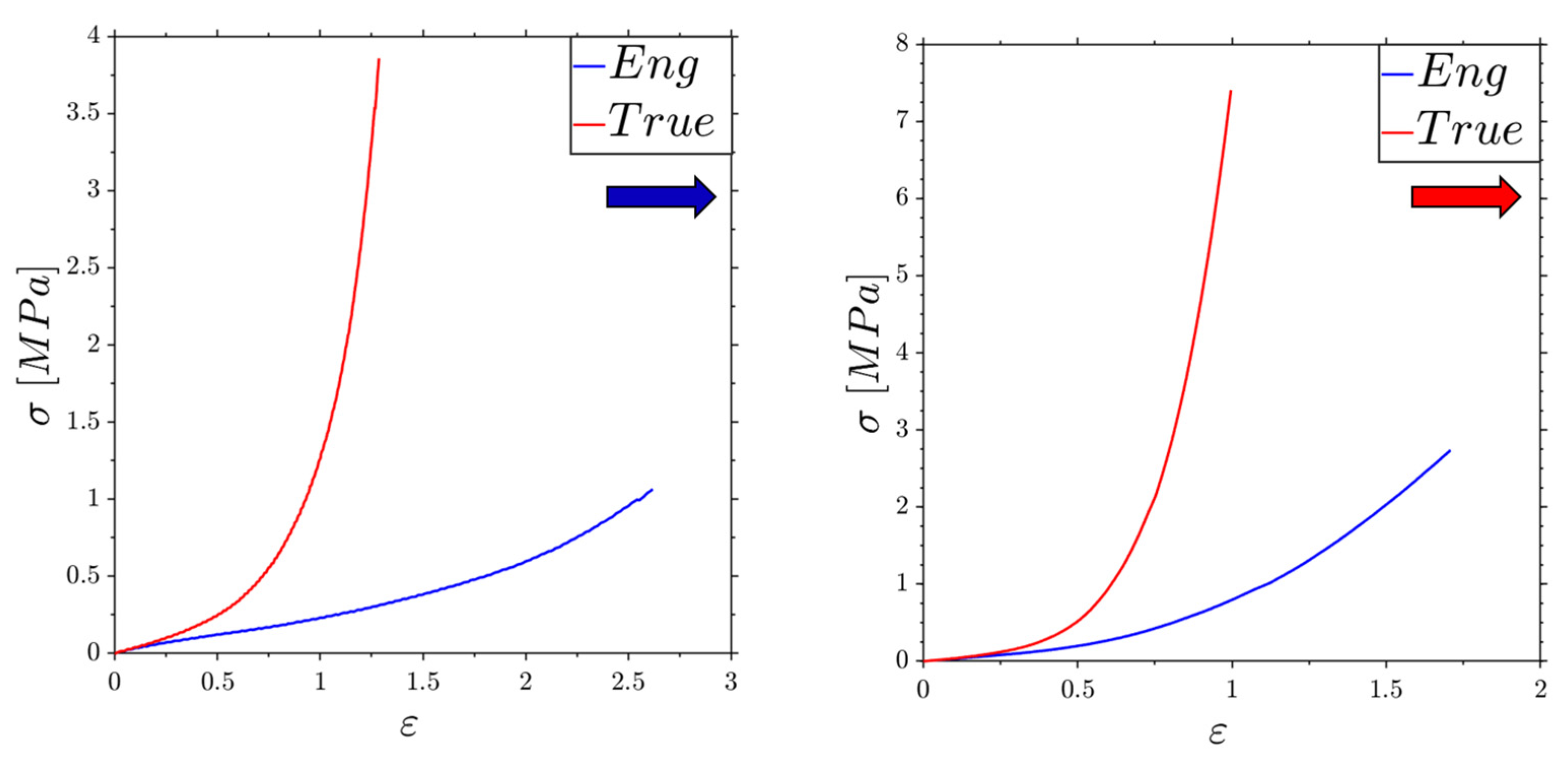
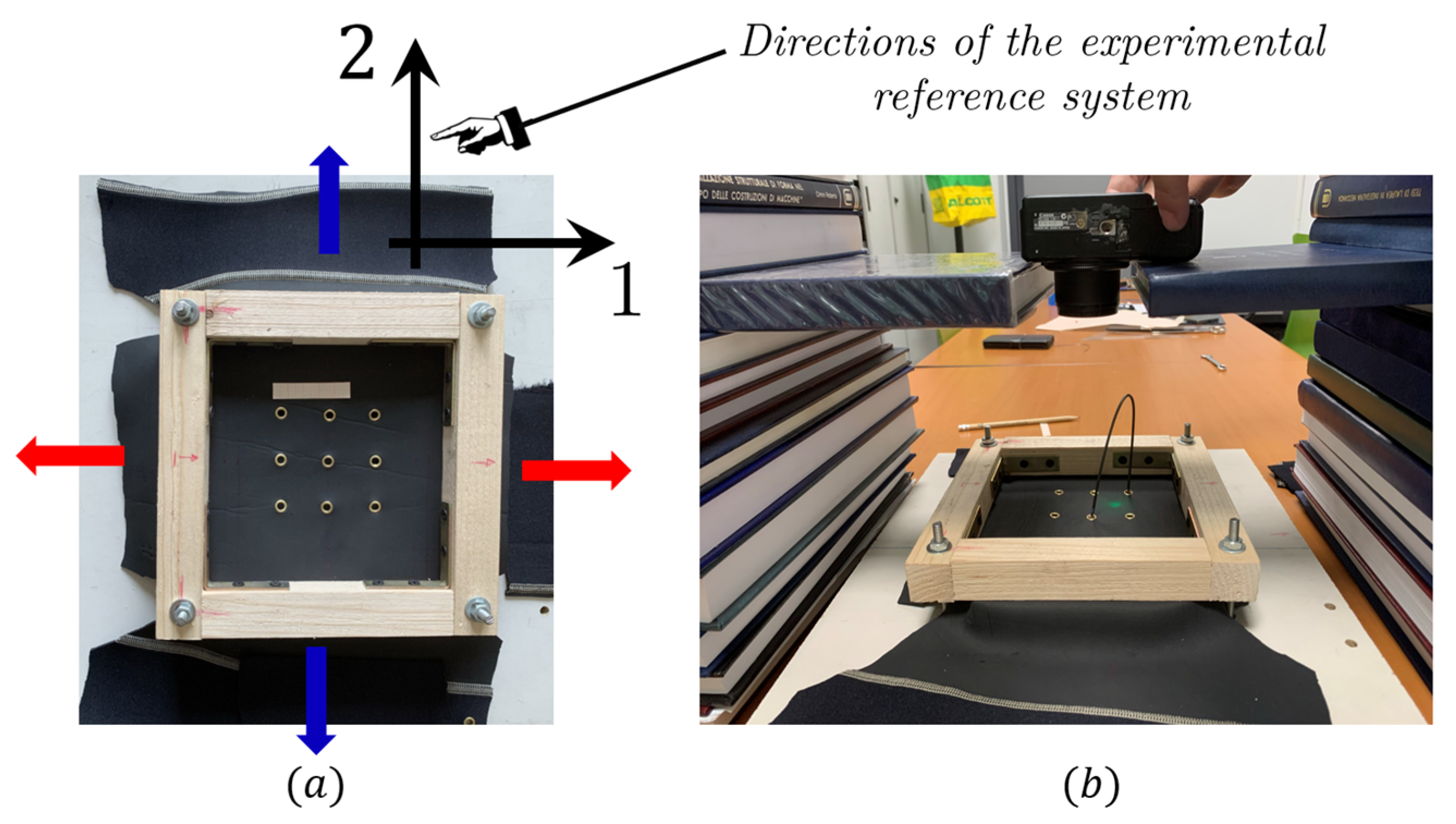
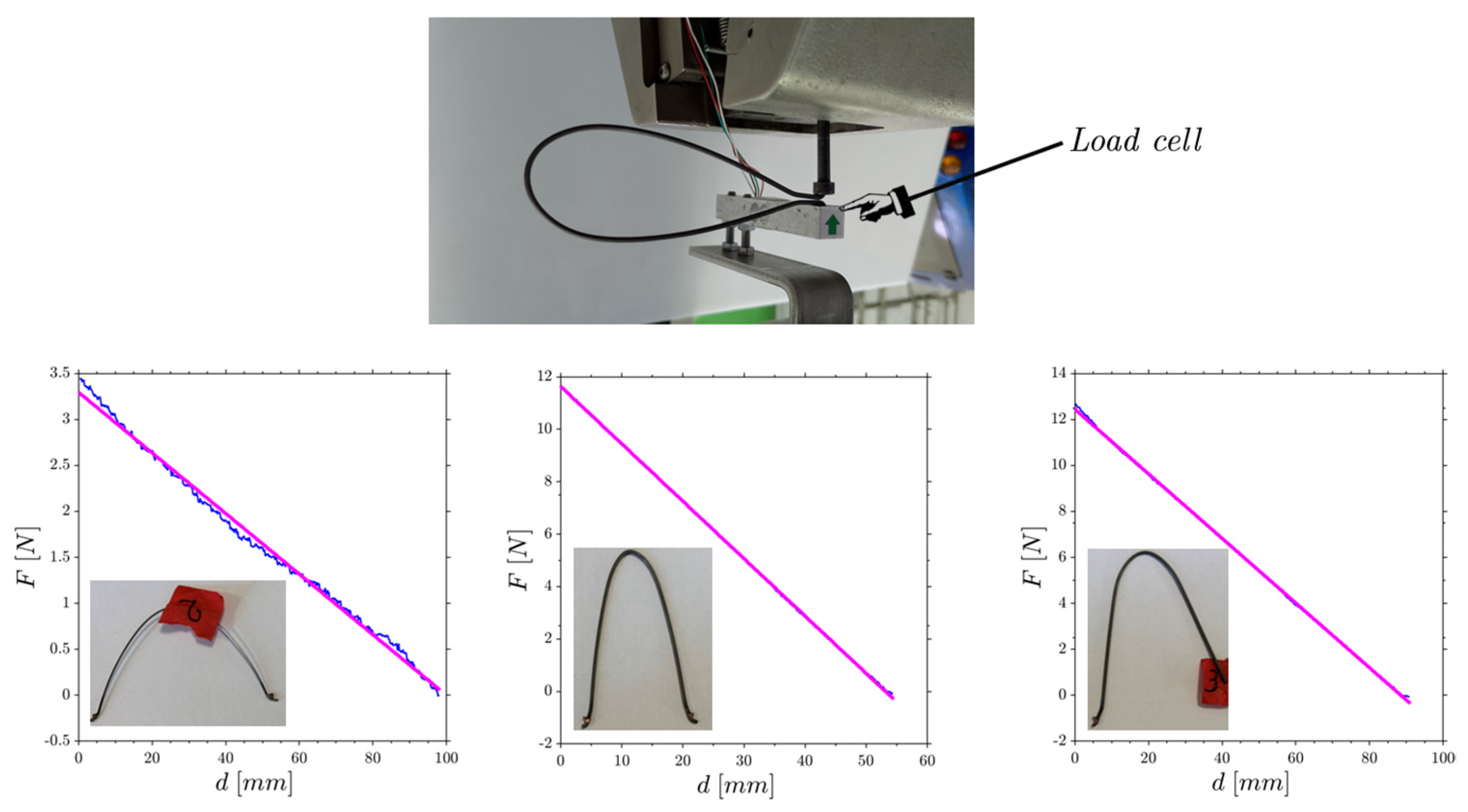
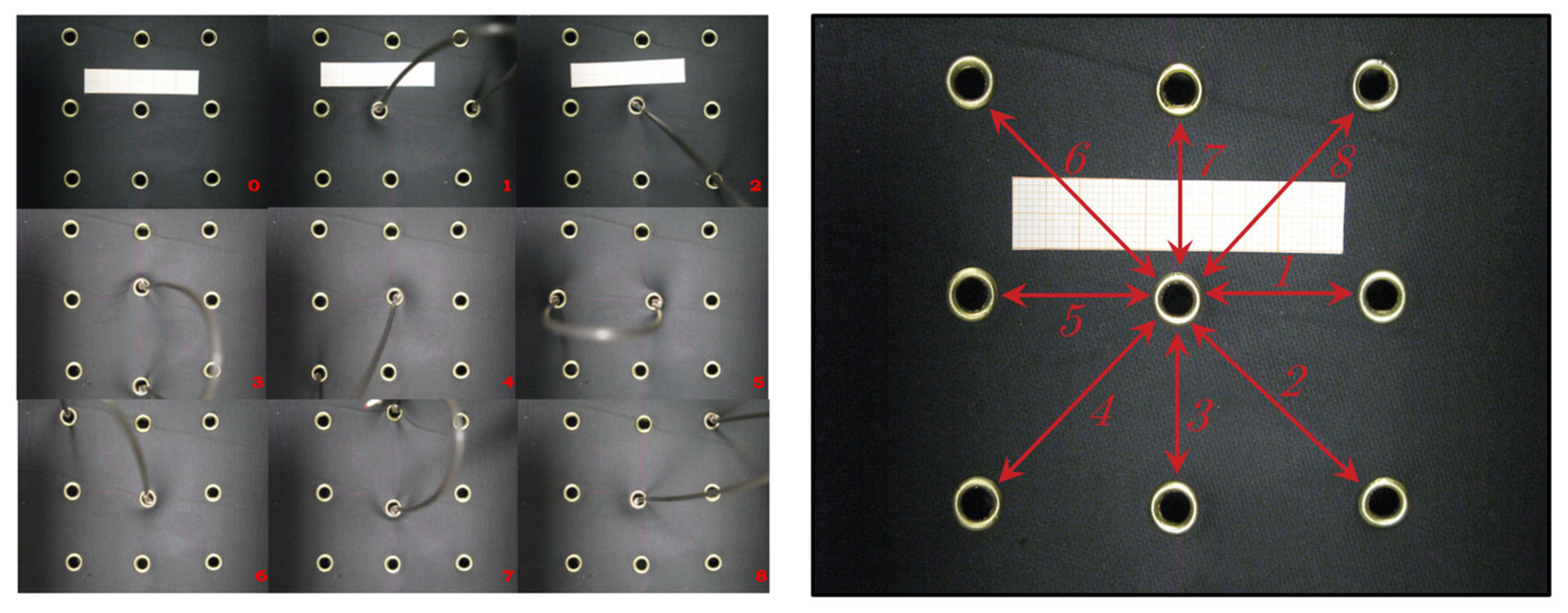
The proposed method was validated through two experimental setups. The first experiment involved a hyperelastic neoprene membrane, which was initially characterized through a tensile test to determine its stiffness. The membrane was then mounted on a wooden frame, and multiple tests were performed under different biaxial preloading conditions. The resulting homogenized secant constitutive matrices provided both the orthotropic elastic matrix and the orientation of the orthotropy reference system. The values obtained for the Young’s moduli, Poisson’s ratios, and shear moduli were consistent with the uniaxial stiffness measured during the tensile test and accurately captured the stiffening behavior in one or the other direction, depending on the applied preloading on the membrane.

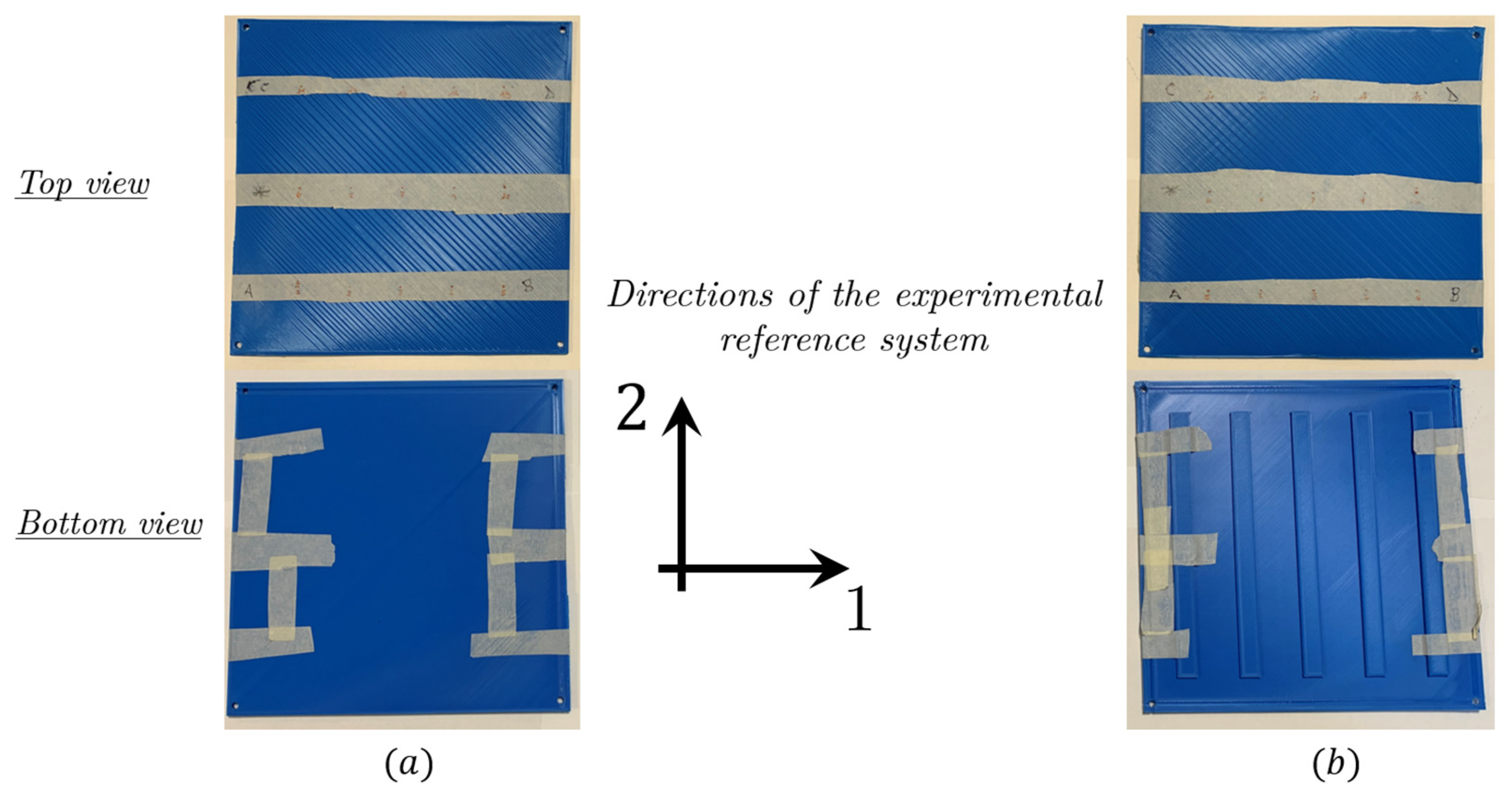
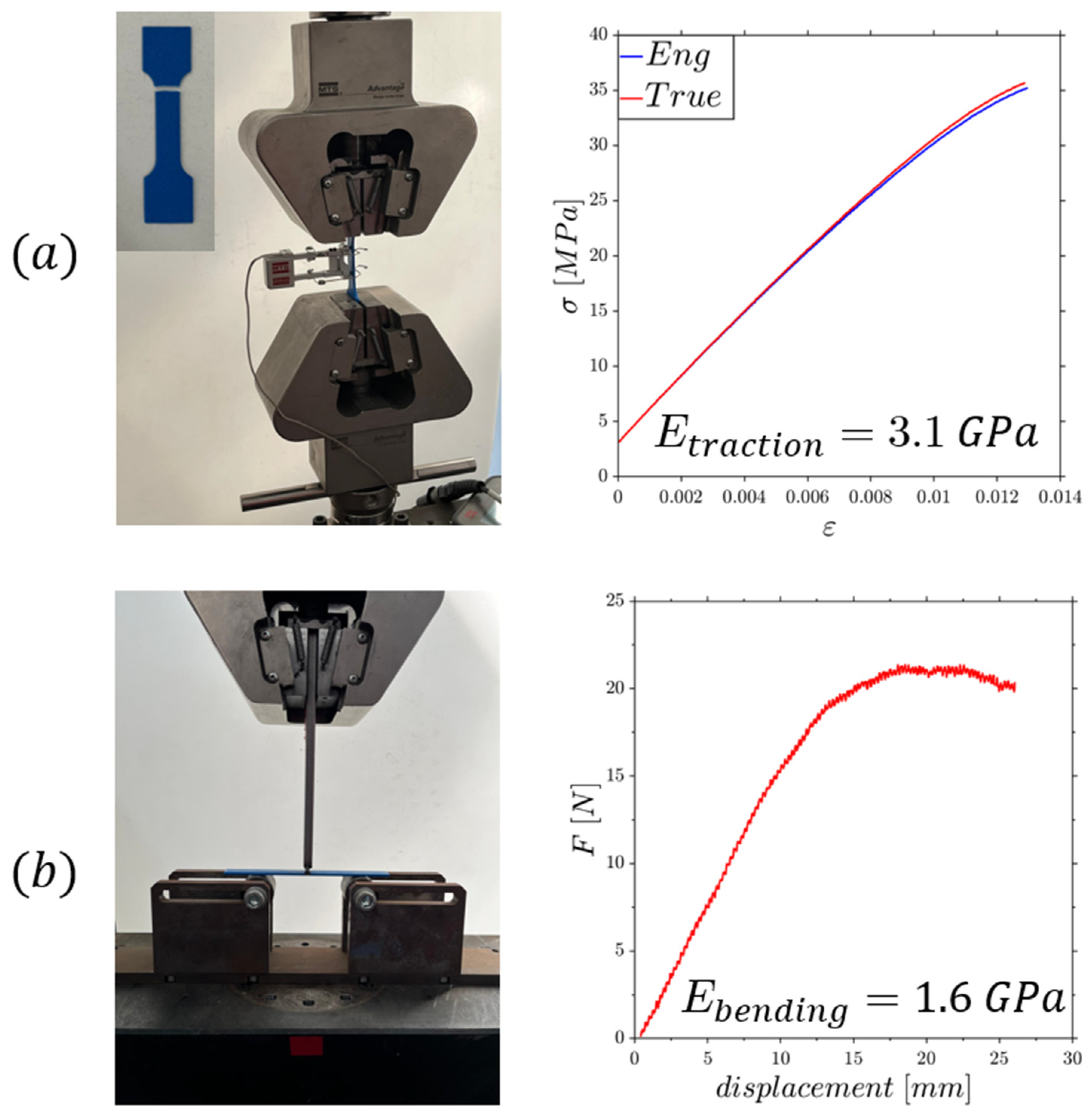
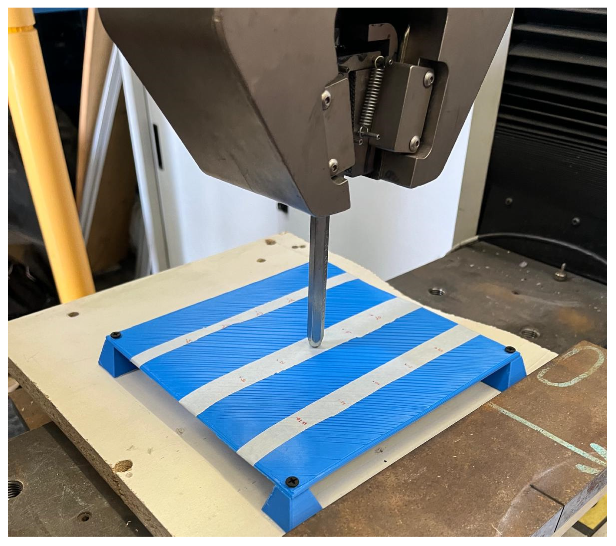
The second test was conducted on PLA plates fabricated through additive manufacturing. Two types of plates were tested: one geometrically homogeneous, and the other featuring reinforcements along one direction, making it geometrically non-homogeneous. The 3D-printed material was first characterized under both tensile and flexural tests. The plates were then clamped at four corners and loaded under displacement-controlled conditions using a compression machine and a load cell. The data processed with the proposed calculation method successfully returned the full elastic constitutive matrix of the material, providing both the orthotropic stiffness parameters and the orientation of the orthotropic reference system. The values of orthotropic stiffness obtained in the two directions were in agreement with the axial stiffness measured during the flexural test and clearly caught the reinforcement effect of the non-homogeneous plate compared with the isotropic one.

Overall, this method was proven to be highly straightforward from an experimental standpoint and is capable of providing comprehensive information regarding the entire elastic constitutive matrix of complex materials. It offers a practical and efficient approach to characterize the anisotropic elastic properties of materials in cases where traditional modeling may be difficult or not applicable.

References

1. Andreassen, E.; Andreasen, C.S. How to determine composite material properties using numerical homogenization. Comput. Mater. Sci. 2014, 83, 488–495. [Google Scholar] [CrossRef]
2. Boso, D.P.; Lefik, M.; Schrefler, B.A. Recent developments in numerical homogenization. Comput. Assist. Mech. Eng. Sci. 2009, 16, 161–183. [Google Scholar]
3. Hollister, S.J.; Kikuchi, N. Comparison of Homogenization and Standard Mechanics Analyses for Periodic Porous Composites. Comput. Mech. 1992, 10, 73–95. [Google Scholar] [CrossRef]
4. Fang, Z.; Sun, W.; Tzeng, J.T. Asymptotic Homogenization and Numerical implementation to Predict the Effective Mechanical Properties for Electromagnetic Composite Conductor. J. Compos. Mater. 2004, 38, 1371–1385. [Google Scholar] [CrossRef]
5. Hashin, Z.; Shtrikman, S. A variational approach to the theory of composite elastic materials. J. Mech. Phys. Solids 1963, 11, 127–140. [Google Scholar] [CrossRef]
6. Hassani, B.; Hinton, E. A Review of Homogenization and Topology Optimization I—Homogenization Theory for Media with Periodic Structure. Comput. Struct. 1998, 69, 707–717. [Google Scholar] [CrossRef]
7. Hassani, B.; Hinton, E. A Review of Homogenization and Topology Optimization II—Analytical and Numerical Solution of Homogenization Equations. Comput. Struct. 1998, 69, 719–738. [Google Scholar] [CrossRef]
8. Berryman, J.G.; Milton, G.W. Microgeometry of random composites and porous-media. J. Phys. D-Appl. Phys. 1988, 21, 87–97. [Google Scholar] [CrossRef]
9. Chen, H.; Kubo, K.Y. Bone three-dimensional microstructural features of the common osteoporotic fracture sites. World J. Orthop. 2014, 5, 486–495. [Google Scholar] [CrossRef] [PubMed]
10. Lu, Y. Computational modelling of bone microstructure. In Computational Modelling of Biomechanics and Biotribology in the Musculoskeletal System; Woodhead Publishing: Cambridge, UK, 2021; pp. 251–256. [Google Scholar] [CrossRef]
11. Almansour, H.; Mohammed, A.; Lounis, Z. Modeling the resilience of aging concrete bridge columns subjected to corrosion and extreme climate events. In Life Cycle Analysis and Assessment in Civil Engineering: Towards an Integrated Vision; CRC Press: Boca Raton, FL, USA, 2018; pp. 251–256. ISBN 9781315228914. [Google Scholar]
12. Coronelli, D.; Gambarova, P. Structural assessment of corroded reinforced concrete beams: Modeling guidelines. J. Struct. Eng. 2004, 130, 1214–1224. [Google Scholar] [CrossRef]
13. Iandiorio, C.; Cafolla, F.; Salvini, P. Homogenized Stiffness Matrix of Two-Node Elements through Experimental Flexibility tests. In IOP Conference Series: Materials Science and Engineering; IOP Publishing: Bristol, UK, 2024; Volume 1306, p. 012039. [Google Scholar] [CrossRef]
14. Iandiorio, C.; Salvini, P. Elastic-plastic analysis with pre-integrated beam finite element based on state diagrams: Elastic-perfectly plastic flow. Eur. J. Mech.-A/Solids 2023, 97, 1214–1224. [Google Scholar] [CrossRef]
15. Iandiorio, C.; Salvini, P. Updated Lagrangian Curvilinear Beam Element for 2D Large Displacement Analysis. In Proceedings of the 5th International Conference on Numerical Modelling in Engineering, Gent, Belgium, 23–24 August 2022; Lecture Notes in Mechanical Engineering. Springer: Singapore, 2023. [Google Scholar] [CrossRef]
16. Gupta, K.K.; Meek, J.L. A brief history of the beginning of the finite element method. Int. J. Numer. Methods Eng. 1996, 39, 3761–3774. [Google Scholar] [CrossRef]
17. Samuelsson, A.; Zienkiewicz, O.C. History of the stiffness method. Int. J. Numer. Methods Eng. 2006, 67, 149–157. [Google Scholar] [CrossRef]
18. Felippa, C.A.; Park, K.C. A direct flexibility method. Comp. Meth. Appl. Mech. Eng. 1997, 149, 319–337. [Google Scholar] [CrossRef]
19. Sadd, M.H. Elasticity: Theory, Applications, and Numerics; Academic Press: Cambridge, MA, USA, 2009; ISBN 978-0323163460. [Google Scholar]
20. Zienkiewicz, O.C.; Taylor, R.L. The Finite Element Method, Solid Mechanics; Wiley: Hoboken, NJ, USA, 2000; Volume 2, ISBN 978-0750650557. [Google Scholar]
21. Przemieniecki, J.S. Finite Element Structural Analysis: New Concepts; Amer Inst of Aeronautics & Astronautics: Reston, VA, USA, 2009; ISBN 978-1563479977. [Google Scholar]
22. Bathe, K.J.; Wilson, E.L. Numerical Methods in Finite Element Analysis; Prentice-Hall: Hoboken, NJ, USA, 1976; ISBN 978-0136271901. [Google Scholar]
23. Iandiorio, C.; Cafolla, F.; Salvini, P. Optimal Uniform Strength Design of Frame and Lattice Structures. Comput. Struct. 2024, 301, 10743024. [Google Scholar] [CrossRef]
24. Iandiorio, C.; Cirelli, M.; Salvini, P.; Valentini, P.P. Elasto-Kinematics and second-order pseudo-rigid model of cross-axis flexure hinges. Mech. Mach. Theory 2025, 205, 105894. [Google Scholar] [CrossRef]
25. Daniel, I.M.; Ishai, O. Engineering Mechanics of Composite Materials; OUP: Oxford, UK, 2005; ISBN 978-0195150971. [Google Scholar]
Figure 1. Plate loaded orthogonally to its plane on a single node (red point).
Engproc 85 00027 g001
Figure 2. Tensile tests on strips of materials taken from orthogonal directions of the diving suit. The blue and red arrows indicate the weak and strong direction according to Figure 3.
Engproc 85 00027 g002
Figure 3. (a) Wooden frame for locking the membrane and adjusting its preloading. (b) Deformation measurement system utilizing digital image acquisition.
Engproc 85 00027 g003
Figure 4. Calibration of the three harmonic steel springs used to load the membrane.
Engproc 85 00027 g004
Figure 5. The eight loading tests conducted on the membrane.
Engproc 85 00027 g005
Figure 6. Mesh composed of 64 four-node plane elements utilized for processing the experimental data.
Engproc 85 00027 g006
Figure 7. Top and bottom views of the non-reinforced plate (a) and reinforced plate (b).
Engproc 85 00027 g007
Figure 8. Tensile test (a) and bending test (b) on the PLA specimens.
Engproc 85 00027 g008
Figure 9. Experimental setup for testing the plates.
Engproc 85 00027 g009
Figure 10. Mesh composed of 34 four-node plate elements utilized to process the experimental data.
Engproc 85 00027 g010