Abstract
This study developed a non-destructive testing (NDT) method using infrared thermography to inspect tubes with holes and slots made by electro-erosion and additive manufacturing. CO2 was used as a tracer gas to verify the opening and evaluate the flow shape from the holes and slots. To improve the signal contrast, a controlled hot background was used as a reference, and infrared cameras monitored the thermal response to detect flow variations caused by different geometries. The tests included different diameters, pitches, and aspect ratios, comparing results between additive manufacturing and electro-erosion under various conditions. Moreover, a preliminary setup using compressed air and inductive heating was developed to assess hole openings by cooling the piece, aiming to eliminate CO2 use. The comparison of results, the post-processing analysis of quantitative indices, and specific thermal features enabled a non-destructive evaluation of the holes by using different technologies, providing an assessment of the opening conditions, outlet, geometry, and flow shape.
1. Introduction
The cooling of complex mechanical components, such as those of gas turbine nozzles, is crucial for enhancing performance and maintenance [1,2,3,4,5]. Advanced cooling systems help to maintain theoretical temperature conditions, increasing component reliability and ensuring structural integrity. Non-destructive techniques can be employed to detect the closure or partial obstruction of cooling holes before the service or during operating conditions [1,2,3,4,5]. This approach allows us to prevent system failures by monitoring overheating in inadequately cooled areas and excessive cooling in others.
In particular, considering the case of turbine blades as real components, film cooling is implemented through openings that extend across the entire surface of the blade. The closure of individual openings during operation can lead to blade failure. Therefore, thorough quality control is typically conducted before delivery.
A modern approach to this quality control is through thermographic transmission measurement, which can reliably detect blocked openings. During the measurement, hot air passes through the turbine blade, and the holes surrounding it are observed with a thermographic camera. In this regard, an R&D work was carried out under the BMWi funding program ZIM, titled “VOLGAST”, by some researchers in the Bundesanstalt für Materialforschung und -prüfung (BAM) [6], and the patent DE102006043339A1 [7] is related to this methodology.
This preliminary work involves an experimental investigation of cooling hole systems, starting with simple geometries such as tubes with holes and slots created by Electrical Discharge Machining (EDM). The study will then extend to advanced processes such as additive manufacturing (AM) technology, specifically using the Laser Powder Bed Fusion process (L-PBF), producing some specimens with similar geometries.
The non-destructive technique used in this work is the infrared thermography (IRT) technique, adopting various sensors and excitation sources [6,7,8,9,10,11,12,13,14,15,16,17,18,19].
An experimental campaign with an innovative setup for tests was carried out using carbon dioxide (CO2), opaque to the infrared spectrum (around 4.3 µm), to assess the total or partial closure of single holes and evaluate the flow shape under different configurations. This involved comparing the behavior of unobstructed holes (normal operating conditions) with partially occluded ones. Additionally, a preliminary investigation using compressed air as the cooling gas explored the potential to differentiate between closed and open holes without the use of CO2, still employing infrared thermography as the non-destructive technique.
2. Material and Methods
2.1. Experimental Setup and Campaign with CO2
Figure 1 shows the experimental setup adopted in this work for the first evaluation of hole integrity and flow evaluation with CO2 and infrared thermography. A controlled-temperature heated panel (A) was used to ensure uniform heating across both space and time (temperature target set at 50 ± 0.2 °C within 10 min). The heated panel was used to create an appropriate thermal contrast in the measurement zone when the gas (CO2) passed through the examined samples (B). For the regulation and measurement of the CO2 flow, a pressure regulator was employed to regulate the inlet pressure, along with a flow regulator (C).
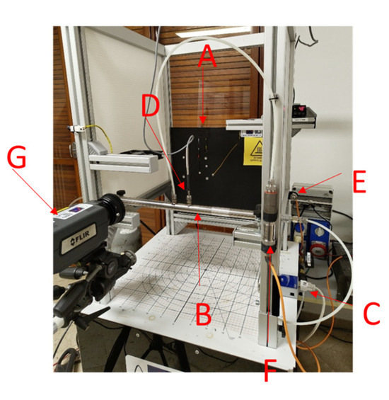
Figure 1.
The setup used to acquire thermal data during the flow tests.
Three different sensors were integrated into the measurement system:
- Ambient temperature (D)
- Absolute pressure (E)
- Gauge pressure (F)
Through the MultiDES system control software IRTA2, developed by DES, it was possible to activate the solenoid valves to allow the passage of CO2 through the circuit. Simultaneously, the acquisition of thermal sequences could be managed through the installed thermal sensor (G), a Teledyne FLIR-cooled A6751 thermal camera (MWIR 3–5 µm, lens 25 mm) equipped with a CO2 filter (CWL: 4300 ± 40 nm; HW: 200 ± 25 nm; Tavg: 87%—transmission; blocking: 190–30,000 nm).
Different specimens (Figure 2) realized in EDM were constructed, considering a complete Design of Experiments (DOE) in which the diameter of the holes and the step between two consecutive holes change; in particular, for each tube, 4 rows of holes per side were realized, for a total of 2 tubes (specimens), 16 arrays, and 96 holes (exit angle 90°). The DOE followed the scheme reported in Table 1.
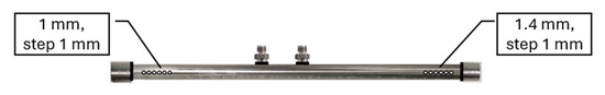
Figure 2.
An example of one of the investigated specimens, featuring two specific arrays of holes, representative of the common geometry of the specimens.

Table 1.
The DOE that summarizes the 16 cases investigated, considering 2 tubes, 16 arrays, and 96 holes (EDM technology).
After different preliminary tests, an experimental campaign of 16 tests, and related replications (5×), was carried out on these configurations, with all the holes open for each array and the others closed using a special aluminum adhesive tape. The tests were carried out at the same fixed gauge pressure level. Table 2 reports the test parameters related to acquisition and boundary flow conditions. The total duration was about 30 s for each test (the steady state conditions were reached in the flow meter after 15 s of testing). To increase the geometrical resolution, specific tests were performed, adding a ring spacer before the lens of the sensor.
Table 2.
Acquisition parameters and boundary flow conditions, EDM tubes and holes.
Considering the additive manufacturing process as an innovative technology to produce cooling holes, some specimens were realized that could be considered real cases and were investigated with the same setup and technique. Some preliminary tests were carried out considering one of the produced specimens (Table 3, 4 cases considering all the holes open) as a representative case of this technology and the problems related to it (trapped powder, different diameters with respect to the intended nominal one, etc.). The same parameters reported in Table 2 were adopted for these tests.
Table 3.
Additive manufacturing (AM) components—hole theoretical diameters and steps between two holes for each array.
2.2. Experimental Setup and Campaign with Compressed Air
As preliminary evaluation, some tests were carried out by means of thermal methods, using compressed air instead of CO2. The adopted setup is shown in Figure 3, including a cooled sensor (FLIR A6751sc, MWIR 3–5 µm, lens 50 mm) and a ZVS inductor (1000 W, 100 kHz) to heat the specimen, bring it to a temperature of about 100 °C, and create a contrast with respect to the compressed air used to cool down the holes. The inductor was controlled by adopting a function generator to define the pulse duration and switching the power supply ON/OFF. The test consisted of heating the specimen to a uniform temperature with the inductor (about 2 min) and then the release of compressed air through the circuit, monitoring the cooling down with an infrared sensor. After some preliminary tests with different pressure values (from 0.5 to 2 bar), a low-pressure setpoint of just 0.5 bar was adopted. A motorized guide was used to move the inductor away from the piece and make the view clear during the cooling phase.
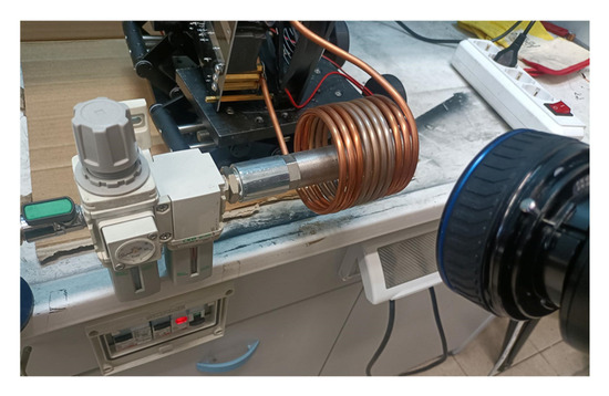
Figure 3.
The setup used to acquire the thermal data during the tests with compressed air.
The adopted test parameters are reported in Table 4. The tests were carried out considering one array and the AM tube.
Table 4.
Setup parameters for tests with compressed air.
3. Procedure for Data Analysis and Preliminary Results
3.1. Data Analysis with CO2
To analyze the acquired raw thermal data, different strategies and algorithms were adopted. The following steps outline the procedure:
- (a)
- Signal Background Evaluation: The signal background was assessed as the mean of 10 frames acquired at the beginning of the test, prior to the application of the CO2 flux.
- (b)
- Steady-State Condition: After reaching steady-state conditions, a thermal sequence of duration 2 s (250 frames) was acquired.
- (c)
- Mean Evaluation: The mean values of the thermal data were computed along the third dimension (time), resulting in a single thermal map.
- (d)
- Background Subtraction: The assessed signal background was subtracted from the mean thermal map calculated in (c).
- (e)
- Cumulative Frame Subtraction: The mean background subtraction (a) point) was applied to each frame of the acquired sequence, and then the resulting frames were summed. The cumulative frame subtraction was an algorithm present in the IRTA 2 software (by DES) that allowed us to enhance the signal to noise ratio.
- (f)
- Applying the PCA algorithm: The Principal Component Analysis (PCA) was based on singular value decomposition algorithm, as described in [14,15,16,17], considering the first component as representative of the obtained results.
Considering a profile at a certain height (350 row) that is the distance from the opening hole in the thermal map (Figure 4, point e), it is possible to obtain a result like the one shown in Figure 4. The obtained result is a peak, which resembles a Gaussian distribution, with a certain amplitude, standard deviation, and area (Table 5). These thermal features were considered for flow evaluation.
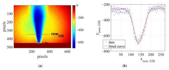
Figure 4.
Schematization of adopted procedure for data analysis: (a) thermal map obtained as synthetic result after cumulative subtraction, profile line 350 (3 mm on flow exit), hole diameter 1 mm; (b) Gaussian fitting of taken profile.
Table 5.
Extracted thermal features from analyzed profile.
Different profiles at different heights (rows) were considered to evaluate the influence of this parameter and the flow behavior near and far from the hole.
To analyze the shape and behavior of a flow, a contour plot of the obtained thermal map (point d) is reported (Figure 5), which visualizes the flow distribution with lines representing equal signal values of the CO2 distribution. The slopes of these lines indicate the direction of the flow: an inclination towards the left or right shows the flow’s directional bias, while the central region may reflect minimal or balanced variation. Different contrast levels between contour lines reveal how sharply the flow changes and its inclination relative to the normal. Comparing slope differences between the left and right sides of the center allows us to identify any asymmetry in the flow. Additionally, the angle between the contour lines and a reference direction provides insights into how the flow orientation aligns with the normal or other directions.
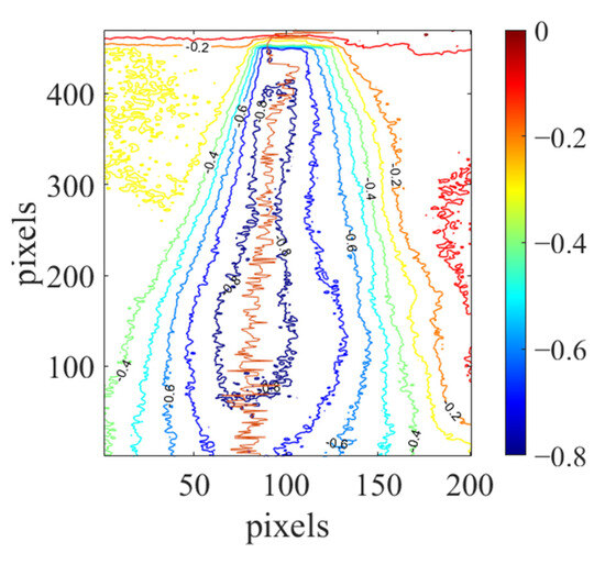
Figure 5.
A contour plot of the obtained result (example related to the previous case, considering the default level number).
3.2. Data Analysis with Compressed Air
To investigate the possibility of recognizing an open or closed hole by means of thermal methods and without CO2 (setup shown in Figure 3), different algorithms were tested during the cooling caused by the introduction of compressed air to the component previously heated to a constant temperature with a thermal inductor. In particular, considering the characteristic cooling behavior of the signal near the hole edges, some algorithms such as a derivative analysis and an analysis of the slope increase with the number of frames at each step, as described in [18,19], were considered. Moreover, different polynomial fittings, repeating the procedure pixel-by-pixel and evaluating the first instants following the introduction of compressed air, were also explored.
4. Results
4.1. Results with CO2
Following the described procedure, the results shown in Figure 6 were obtained for an array of six holes, using cumulative subtraction and the previously detailed analysis parameters. Figure 6a demonstrates a smooth and nearly perpendicular flow from the jet exit for each hole.
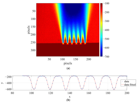
Figure 6.
Results after cumulative subtraction. Case with hole diameter 0.7 mm and step 1.5 mm: (a) map and (b) profile plot at the height/row highlighted with dotted line in (a).
A quantitative analysis was then carried out by examining each hole’s flow individually, separating the different peaks, and fitting the data with a Gaussian profile (Figure 6b). After a signal rescaling with respect to the background (subtraction of the absolute minimum value related to the different profiles and the absolute value of the obtained result), the results, summarized in Table 6, show very similar amplitudes, standard deviations, and area values, confirming the homogeneity of the flow behavior across the array of holes.
Table 6.
A Gaussian fitting, considering the results reported in Figure 6, for a case with a hole diameter of 0.7 mm and a step of 1.5 mm.
Similar results can be obtained in the case of the analyses of different arrays with different diameters (same step between the holes). An example is reported in Figure 7, in which all the holes are open (same pressure, different flow readings), but have different diameters.
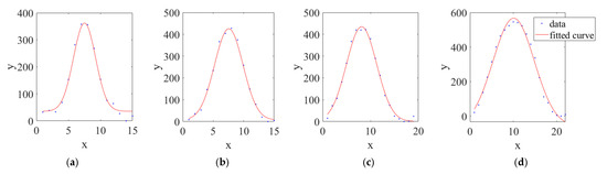
Figure 7.
Results after cumulative subtraction for array with same step (1.5 mm) but different diameters: (a) diameter 0.5 mm, (b) diameter 0.7 mm, (c) diameter 1 mm, (d) diameter 1.4 mm.
The quantitative results are presented in Table 7. As expected, significant differences were observed, particularly in correlation with the hole diameter. This is especially evident for the analysis of the thermal features related to the sigma of the Gaussian profile.
Table 7.
Gaussian fitting, considering results reported in Figure 7, for arrays with different diameters but same step.
When analyzing the additive manufacturing specimens, the behavior often differed significantly from that observed for holes manufactured using EDM. It was common to find holes where the flow was tilted with respect to the vertical direction, as illustrated by the results in Figure 8 (hole diameter 0.9 mm, step 2.2 mm). The data shown in Figure 8a were analyzed using the same algorithm and analysis time as before. These results, along with the contour plot in Figure 8b, confirm that the flow was not homogeneous. Specifically, the flow from the first hole has a significantly lower intensity than the other five (indicated by the absence of the 0.4 level). Unlike the EDM case, the jets do not converge into a single flow at the upper part but instead couple in pairs. The slopes of the various jets (dashed black lines in Figure 8a) generally lean to the right. To verify this behavior and rule out any dependency on boundary conditions, such as the possible presence of an unexpected lateral air jet, the test was repeated on the left side, yielding very similar results.
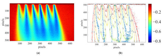
Figure 8.
Results obtained considering analysis of AM specimen—case with hole diameter 0.9 mm and step 2.2 mm: (a) map related to analysis after frame subtraction, with dotted lines that highlight the slope of the flux and (b) contour plot.
As a synthetic and quantitative result, the slope corresponding to the absolute values of the minimum flow level for each jet is presented in Table 8, confirming the previously discussed qualitative results. This slope was determined by fitting a straight line to the blue contours shown in Figure 8b (from row 500, up to row 200). Additionally, the minimum flow value for each hole, representing the maximum intensity in each case, is also reported in the same table. Hole 1 shows, as expected, the lowest intensity value.
Table 8.
A Gaussian fitting, considering the results reported in Figure 8b, for the analysis of an array of an AM specimen.
Additionally, a powder residue was observed around the holes, specifically in the area with the highest absolute signal value near the jet region. Generally, for all the holes, the presence of residual powder influences the flow, resulting in a lower intensity around the area where the jet begins.
4.2. Results with Compressed Air
Figure 9a shows the thermal behavior of the specimen as it cools down, starting when the thermal inductor is no longer above the hot surface and the compressed air valve is opened. Figure 9b focuses on the analysis of the first few frames immediately following the cooling process. Specifically, only the initial 0.2 s, corresponding to 22 frames, were analyzed after the injection of compressed air into the specimen. The frame captured just after the coil was switched off was subtracted as a reference, and the slope in a double-linear scale was assessed. This analysis reveals a significant difference in the signal around the hole, attributed to the cooling effect of the compressed air in these localized areas. These results confirm that all the holes in this specimen were nominally open, consistent with previous data obtained using CO2 as the primary flow. The holes located at the extreme positions (marked as 1 and 6) suffer from boundary conditions effect and exhibit a lower cooling slope.
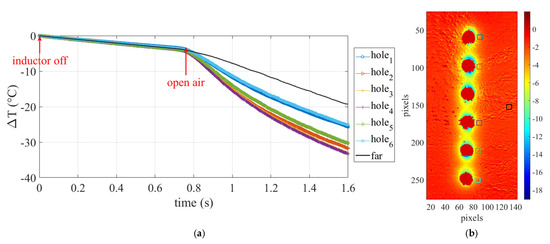
Figure 9.
AM specimen analysis with compressed air; (a) delta temperature over time in different ROI near the holes and far from the flux of compressed air and (b) slope (linear scale) considering analysis of 22 frames (0.2 s) after flux of compressed air.
5. Conclusions and Outlooks
The obtained results demonstrate the effectiveness of thermal methods in evaluating the flow behavior across various configurations, using CO2 as a tracer gas. This study analyzed different scenarios, including traditional EDM processes used for producing cooling holes and innovative technologies such as additive manufacturing. A comprehensive experimental campaign was conducted to assess the influence of hole diameter and spacing (i.e., the distance between consecutive holes) using an innovative setup where the fluid itself was the object of measurement. Various strategies, post-processing algorithms, and thermal features were identified to characterize the flow under different conditions and from multiple perspectives.
A qualitative analysis of the results provides insights into the inclination with respect to the vertical direction and the shape of the flow. In contrast, the extracted thermal features and specific profile analyses offer a quantitative assessment of flow behavior. The analysis of the additive manufacturing results reveals both qualitative and quantitative information about residual powder around the holes and deviations in flow inclination from a perfectly perpendicular condition.
A preliminary investigation using compressed air as the cooling fluid further demonstrated that thermal methods can effectively demonstrate an open-hole condition without the need for CO2.
Future works will explore the extraction of additional thermal features to describe flow behavior using thermal methods in both configurations. This will include the analysis of similar and other specific tubes, as well as real components produced through AM and EDM, featuring more complex geometries with open and closed holes and slots of varying aspect ratios.
Author Contributions
Conceptualization, E.D. and U.G.; methodology, E.D., F.A., M.P., A.G., L.A., D.P. and U.G.; software, G.S. and E.D.; validation, E.D., M.P. and A.G.; formal analysis, E.D., F.A., G.M. and M.P.; investigation, E.D., F.A., G.S. and M.P.; resources, M.P., A.G., L.A. and U.G.; data curation, E.D.; writing—original draft preparation, E.D.; writing—review and editing, F.A., G.M., D.P., U.G. and A.G.; supervision, U.G.; project administration, M.P., A.G., L.A. and U.G.; funding acquisition, M.P., A.G., L.A. and U.G. All authors have read and agreed to the published version of the manuscript.
Funding
This research was supported by the external grant between Politecnico di Bari and Nuovo Pignone Baker Hughes (BH) titled “The assessment of the effectiveness of the nozzle cooling system by non-destructive testing based on thermographic techniques” (scientific responsible Prof. Umberto Galietti).
Institutional Review Board Statement
Not applicable.
Informed Consent Statement
Not applicable.
Data Availability Statement
The data are available upon motivated request to the corresponding author.
Conflicts of Interest
The authors declare no conflicts of interest.
References
- Li, Z.Y.; Wei, X.T.; Guo, Y.B.; Sealy, M.P. State-of-art, challenges, and outlook on manufacturing of cooling holes for turbine blades. Mach. Sci. Technol. 2015, 19, 361–399. [Google Scholar] [CrossRef]
- Swaminathan, V.P.; Allen, J.M. Surface degradation and cracking in combustion turbine blade cooling passages. Mater. Manuf. Process 1995, 10, 867–885. [Google Scholar] [CrossRef]
- Chowdhury, T.S.; Mohsin, F.T.; Tonni, M.M.; Mita MN, H.; Ehsan, M.M. A critical review on gas turbine cooling performance and failure analysis of turbine blades. Int. J. Thermofluids 2023, 18, 100329. [Google Scholar] [CrossRef]
- Ozaner, O.C.; Karabulut, Ş.; Izciler, M. Study of the surface integrity and mechanical properties of turbine blade fir trees manufactured in Inconel 939 using laser powder bed fusion. J. Manuf. Process. 2022, 79, 47–59. [Google Scholar] [CrossRef]
- Tinga, T.; Van Kampen, J.F.; De Jager, B.; Kok, J.B. Gas turbine combustor liner life assessment using a combined fluid/structural approach. J. Eng. Gas Turbines Power. 2007, 129, 69–79. [Google Scholar] [CrossRef]
- Doroshtnasir, M.; Krankenhagen, R.; Maierhofer, C.; Block, N.; Binder, P. Volumenstrombestimmung an gasdurchflossenen Düsen mit Thermografie. In Proceedings of the DACH-Jahrestagung 2012-ZfP in Forschung, Entwicklung und Anwendung, Graz, Austria, 17–19 September 2012; No. DGZfP-BB 136. p. Poster-34. [Google Scholar]
- Goldammer, M.; Heinrich, W.D. Method and Device for Determining Component Parameters by Means of Thermography. Patent DE102006043339A1, 11 November 2010. [Google Scholar]
- Jonsson, I.; Chernoray, V.; Dhanasegaran, R. Infrared thermography investigation of heat transfer on outlet guide vanes in a turbine rear structure. Int. J. Turbomach. Propuls. Power 2020, 5, 23. [Google Scholar] [CrossRef]
- Simon, B.; Filius, A.; Tropea, C.; Grundmann, S. IR thermography for dynamic detection of laminar-turbulent transition. Exp. Fluids 2016, 57, 93. [Google Scholar] [CrossRef]
- Gardner, A.D.; Eder, C.; Wolf, C.C.; Raffel, M. Analysis of differential infrared thermography for boundary layer transition detection. Exp. Fluids 2017, 58, 122. [Google Scholar] [CrossRef]
- Carlomagno, G.M.; Cardone, G. Infrared thermography for convective heat transfer measurements. Exp. Fluids 2010, 49, 1187–1218. [Google Scholar] [CrossRef]
- Carlomagno, G.M.; Cardone, G.; Meola, C.; Astarita, T. Infrared thermography as a tool for thermal surface flow visualization. J. Vis. 1998, 1, 37–50. [Google Scholar] [CrossRef]
- Astarita, T.; Cardone, G.; Carlomagno, G.M. Infrared thermography: An optical method in heat transfer and fluid flow visualisation. Opt. Lasers Eng. 2006, 44, 261–281. [Google Scholar] [CrossRef]
- Rajic, N. Principal Component Thermography; Defence Science and Technology Organisation: Melbourne, Australia, 2002. [Google Scholar]
- Omar, M.A.; Parvataneni, R.; Zhou, Y. A combined approach of self-referencing and Principle Component Thermography for transient, steady, and selective heating scenarios. Infrared Phys. Technol. 2010, 53, 358–362. [Google Scholar] [CrossRef]
- D’Accardi, E.; Palumbo, D.; Galietti, U. Experimental procedure to assess depth and size of defects with pulsed thermography. J. Nondestruct. Eval. 2022, 41, 41. [Google Scholar] [CrossRef]
- Feuillet, V.; Ibos, L.; Fois, M.; Dumoulin, J.; Candau, Y. Defect detection and characterization in composite materials using square pulse thermography coupled with singular value decomposition analysis and thermal quadrupole modeling. NDT E Int. 2012, 51, 58–67. [Google Scholar] [CrossRef]
- Dell’Avvocato, G.; Palumbo, D. Thermographic procedure for the assessment of Resistance Projection Welds (RPW): Investigating parameters and mechanical performances. J. Adv. Join. Process. 2024, 9, 100177. [Google Scholar] [CrossRef]
- D’Accardi, E.; De Finis, R.; Dell’Avvocato, G.; Masciopinto, G.; Palumbo, D.; Galietti, U. Conduction thermography for non-destructive assessment of fatigue cracks in metallic materials. Infrared Phys. Technol. 2024, 140, 105394. [Google Scholar] [CrossRef]
Disclaimer/Publisher’s Note: The statements, opinions and data contained in all publications are solely those of the individual author(s) and contributor(s) and not of MDPI and/or the editor(s). MDPI and/or the editor(s) disclaim responsibility for any injury to people or property resulting from any ideas, methods, instructions or products referred to in the content. |
© 2025 by the authors. Licensee MDPI, Basel, Switzerland. This article is an open access article distributed under the terms and conditions of the Creative Commons Attribution (CC BY) license (https://creativecommons.org/licenses/by/4.0/).