Structural Health-Monitoring Strategy Based on Adaptive Kalman Filtering ^†

Abstract

Structures are exposed to aging and extreme events that can decrease the relevant safety margins or even lead to (partial) collapse mechanisms under unforeseen loading conditions. Structural health monitoring (SHM) therefore appears to be compulsory to avoid accidents by tracking the evolution of the state of the system and sending out warnings as soon as critical conditions are met or drifts from the response of the undamaged structure are identified. One of the approaches to online SHM rests on Kalman filtering, which is able to build the time evolution of the structural state upon the Bayes’ rule. In a customary joint version of the filtering procedure, state variables and health parameters are joined together in an extended state vector; while state variables, e.g., lateral displacements of shear buildings, can be observed thanks to pervasive sensor networks, the health parameters usually linked to the structural stiffness cannot, leading to possible divergence issues characterized by biases in the estimates. These issues are further enhanced by difficulties in setting the covariance terms, whose initialization is required to utilize Kalman filters. In this work, we investigate an adaptive strategy to the online tuning of the aforementioned covariance terms, leading to an improvement of the filter outcomes without issues related to its instability. This procedure is then applied to the SHM of a shear building, to highlight the excellent results in terms of accuracy and robustness.

1. Introduction

Structural health monitoring (SHM) plays a vital role in ensuring the safety, reliability, and longevity of large-scale structures such as bridges, buildings, dams, and wind turbines. It involves the continuous monitoring and assessment of the structural integrity to detect potential defects, damages, or anomalies. Traditional SHM approaches rely on periodic inspections, which may not provide real-time insights into structural health and may lead to the delayed detection of critical issues. The global structural health monitoring market size was valued at USD 2210 million in 2021 and is projected to reach USD 7595 million by 2030, growing at a compound annual growth rate of 14.7% during the forecast period [1].

The Extended Kalman Filter (EKF) can simultaneously estimate both structural properties, such as the interstory stiffness in a shear building, and state by extending the state vector [2,3]. However, the EKF assumes complete knowledge of the process noise covariance and measurement noise covariance matrices, which is difficult to foresee in most cases and this significantly affects the accuracy of estimations. To estimate the process and measurement noise covariances, approaches based on adaptive filtering have been proposed, e.g., by Mehra [4].

In this paper, an adaptive strategy is adopted in conjunction with the EKF on a two-story shear building, aiming to automatically tune the process noise covariance and improve the accuracy and stability of the estimation of the structural stiffness and, therefore, health. The general conclusion is that the Adaptive Extended Kalman Filter (AEKF) not only outperforms the traditional EKF in accuracy, but also demonstrates robustness in multi-parameter estimation and damage detection.

The remainder of the contribution is arranged as follows. Section 2 discusses the structural model and the adaptive Kalman filtering theory applied here. In Section 3, numerical outcomes and estimations by the Kalman filtering procedure are presented to validate the advantages of the AEKF. In Section 4, some final conclusions are drawn along with further proposed enhancements to deal with realistic structural systems.

2. Materials and Methods

2.1. Structural Model and Data Generation

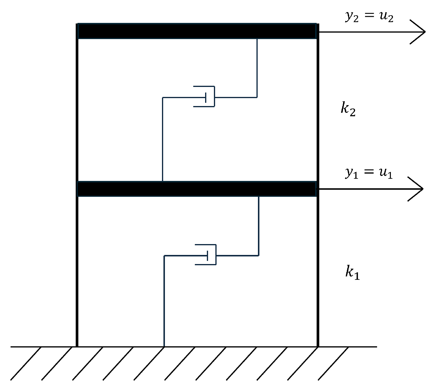
The considered structure is the two-story shear building shown in Figure 1. Measurement of the lateral displacements of the first and second stories are collected every 0.01 s and are adopted as observations for the Kalman filter. Exploiting the recorded earthquake input employed in [5], the structure is subjected to the relevant equivalent forces over a duration of 40.96 s. An explicit Newmark time integration scheme [6] is employed to generate the pseudo-experimental evolution of the state of the structure via a MATLAB code. The interstory stiffnesses $k_1$ and $k_2$ have to be identified or tuned during the analysis, and may even change in time due to some damage accumulation processes which are indeed not explicitly modeled due to a time-scale separation principle (see [7,8]).

2.2. Extended Kalman Filter

The EKF, see [9,10,11,12,13,14,15,16,17], operates on the structural system through the state transition equation:

$${\mathbf{x}}_k=\mathbf{f}\left({\mathbf{x}}_{k-1}\right)+{\mathbf{w}}_k,$$

(1)

and the measurement equation:

$${\mathbf{z}}_k=\mathbf{H}{\mathbf{x}}_k+{\mathbf{v}}_k,$$

(2)

where the following definitions apply:

• ${\mathbf{x}}_k$ is the state vector at time $t_k$, including, in our analysis, displacements, velocities, accelerations, and interstory stiffness values.
• ${\mathbf{z}}_k$ is the measurement vector at time $t_k$ consisting of the lateral displacements of the two stories.
• $\mathbf{f}(·)$ is the state transition function, linked to the adopted Newmark time integration procedure. It must be noted that the response of the system is linear, but the operator $\mathbf{f}$ becomes nonlinear due to the inclusion of the stiffness terms in the state vector. Details can be found in Appendix A.
• $\mathbf{H}$ is the observation matrix, describing the relationship between measurements and the state. In this case, it is a Boolean matrix with non-zero entries to select the observed displacements out of the state vector.
• ${\mathbf{w}}_k$ is the process noise, a zero-mean Gaussian process with covariance ${\mathbf{Q}}_k$.
• ${\mathbf{v}}_k$ is the measurement noise, a zero-mean Gaussian process with covariance ${\mathbf{R}}_k$.

The EKF can be decomposed into 3 main steps:

• Initialization
  It sets the initial guess for the state ${\widehat{\mathbf{x}}}_{0|0}$ and error covariance ${\mathbf{P}}_{0|0}$.
• Prediction
  The estimate of the predicted state is moved forward in time according to

  $${\widehat{\mathbf{x}}}_{k|k-1}=\mathbf{f}\left({\widehat{\mathbf{x}}}_{k-1|k-1}\right);$$

  (3)

  and, if the state transition Jacobian is

  $${\mathbf{F}}_{k-1}={\left.{\displaystyle \frac{\partial \mathbf{f}}{\partial \mathbf{x}}}\right|}_{{\widehat{\mathbf{x}}}_{k-1|k-1}}.$$

  (4)

  then the predicted error covariance reads as

  $${\mathbf{P}}_{k|k-1}={\mathbf{F}}_{k-1}{\mathbf{P}}_{k-1|k-1}{\mathbf{F}}_{k-1}^{\top }+{\mathbf{Q}}_{k-1}.$$

  (5)

  with ${·}^{\top }$ standing for transpose.
• Update
  By exploiting the innovation or measurement residuals, defined as the difference between measurements and prediction from the last step according to

  $${\mathbf{y}}_k={\mathbf{z}}_k-\mathbf{H}{\widehat{\mathbf{x}}}_{k|k-1};$$

  (6)
  The innovation covariance can be obtained as

  $${\mathbf{S}}_k=\mathbf{H}{\mathbf{P}}_{k|k-1}{\mathbf{H}}^{\top }+{\mathbf{R}}_k,$$

  (7)

  and the Kalman gain reads as

  $${\mathbf{K}}_k={\mathbf{P}}_{k|k-1}{\mathbf{H}}^{\top }{\mathbf{S}}_k^{-1}.$$

  (8)
  The updated state estimate is retrieved as

  $${\widehat{\mathbf{x}}}_{k|k}={\widehat{\mathbf{x}}}_{k|k-1}+{\mathbf{K}}_k{\mathbf{y}}_k,$$

  (9)

  and the updated error covariance is

  $${\mathbf{P}}_{k|k}=(\mathbf{I}-{\mathbf{K}}_k\mathbf{H}){\mathbf{P}}_{k|k-1}.$$

  (10)

2.3. Adaptive Extended Kalman Filter

In Kalman filtering, it is usually assumed that the process noise covariance and the measurement noise covariance are known in advance, or can be tuned beforehand on the basis of a trial-and-error procedure. They thus represent a kind of hyperparameters of the numerical procedure. This can be true for ${\mathbf{R}}_k$, as it is related to the noise level of the measurements and so can be determined from the technical features of the measurement equipment, but it is certainly not for ${\mathbf{Q}}_k$. An improper selection of ${\mathbf{Q}}_k$ can lead to significant errors in state estimation, so an adaptive strategy for estimating ${\mathbf{Q}}_k$ and $\mathbf{R}$ based on the innovation sequence is reported here; see also [18].

Specifically, the process noise covariance can be recursively updated by way of the expected value of the innovation, according to

$${\mathbf{Q}}_{k-1}={\mathbf{K}}_k\mathbb{E}\left[{\mathbf{y}}_k{\mathbf{y}}_k^{\top }\right]{\mathbf{K}}_{\mathbf{k}}^{\mathbf{T}}$$

(11)

where $\mathbb{E}\left[{\mathbf{y}}_k{\mathbf{y}}_k^{\top }\right]$ is usually computed by averaging all the innovation terms at each step of filtering. A so-called forgetting factor $\alpha$ (see also [19]) is used to weight the innovation [18,20], so that the estimation of ${\mathbf{Q}}_k$ over time is

$${\mathbf{Q}}_k=\alpha {\mathbf{Q}}_{k-1}+(1-\alpha )\left({\mathbf{K}}_k{\mathbf{y}}_k{\mathbf{y}}_k^{\top }{\mathbf{K}}_k^{\top }\right)$$

(12)

The value of $\alpha$ obviously affects the rate of estimation change. In this work, after a preliminary parametric investigation, $\alpha$ has been set to $0.6$ to attain a robust and reliable performance.

3. Results

In this study, the AEKF is compared with the traditional EKF in terms of accuracy of estimations of the interstory stiffness(es) of the shear building of Figure 1. In the analysis, the process noise covariance matrix is randomly initialized to possibly avoid any bias induced by the initial expert guess. First, a single parameter is tuned by assuming that the interstory stiffness is constant for the building. Next, to investigate the capability of AEKF to handle a multi-parameter estimation problem, a different value of the stiffness is adopted for each interstory. Finally, to also assess the capability of AEKF to promptly react to changes in the structural health, departing from the second case, a reduction of one stiffness is introduced in the analysis so that the estimation becomes a truly time-dependent problem solution.

In the absence of an accurate know-how in terms of health parameters, the AEKF is shown to be able to automatically adjust the stiffness terms based on the innovation sequence, yielding high-accuracy estimations of both states and structural health. To demonstrate the effectiveness of the AEKF, the results obtained in the three scenarios described above are presented in the following.

3.1. Scenario 1: Single Stiffness Parameter

In this case, the two interstory stiffness values $k_1$ and $k_2$ are assumed to be the same, namely $k_1=k_2=1.4\times {10}^9$ N/m. To provide a fair comparison, the filters are initialized with the same state estimate and error covariance matrix, as well as the same process and measurement noise covariance matrices, adopting the following:

$$\begin{array}{cc}\hfill {\widehat{\mathbf{x}}}_{0|0}& ={\left[\begin{array}{ccccccc}0& 0& 0& 0& 0& 0& 1\times {10}^9\end{array}\right]}^{\top }\hfill \\ \hfill {\mathbf{P}}_{0|0}& =diag(\underset{6\mathrm{times}}{\underbrace{1\times {10}^{-10},\cdots ,1\times {10}^{-10}}},1\times {10}^{14})\hfill \\ \hfill {\mathbf{Q}}_0& =diag(\underset{6\mathrm{times}}{\underbrace{1\times {10}^{-4},\cdots ,1\times {10}^{-4}}},1\times {10}^{12})\hfill \\ \hfill {\mathbf{R}}_0& =diag(8.6\times {10}^{-9},2.2\times {10}^{-8},6.3\times {10}^{-6},1.6\times {10}^{-5},5.3\times {10}^{-3},1.4\times {10}^{-2},1\times {10}^{16})\hfill \end{array}$$

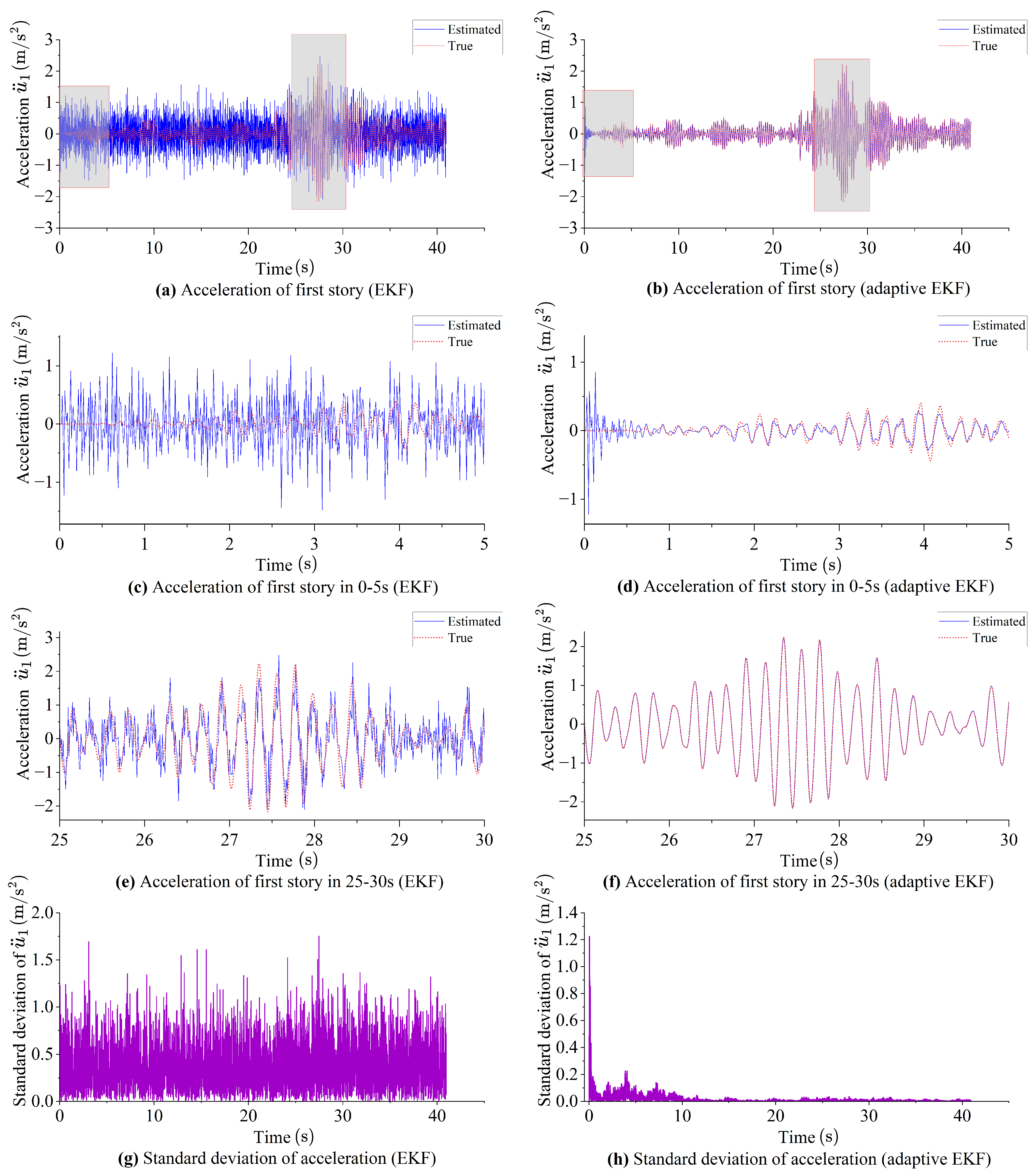
The AEKF shows a superior performance in relation to the estimates of all the structural state components (displacements $\mathbf{u}$, velocities $\dot{\mathbf{u}}$, and accelerations $\ddot{\mathbf{u}}$). As exemplary results, the time histories of the acceleration estimates for the first story are compared in Figure 2 to illustrate the difference between the filters’ outcomes. When provided with an inaccurate initial process noise covariance matrix, it is reported that the error in ${\ddot{u}}_1$ given by the EKF does not decrease in 40.96 s. In contrast, the AEKF provides an error in ${\ddot{u}}_1$ that diminishes to nearly zero within 10 s, with the estimation remaining consistently convergent with the true value thereafter.

Regarding the estimation of the stiffness, as shown in Figure 3, the traditional EKF performs poorly compared to the AEKF when an inappropriate process noise covariance is provided. In the EKF, the estimation of the stiffness shows negligible changes and maintains a significant bias away from the true value. In contrast, the AEKF leads to an estimation of stiffness that converges to the true value within 10 s, and further reduces the error over the remaining time.

The initial process noise covariance ${\mathbf{Q}}_0$ is set as diagonal, with entries, respectively, referring to the story displacements, velocities, and acceleration, and to the interstory stiffness. The matrix ${\mathbf{Q}}_{\mathrm{final}}$ reads

$${\mathbf{Q}}_{\mathrm{final}}={\left[\begin{array}{ccccccc}9\times {10}^{-12}& 1\times {10}^{-11}& -3\times {10}^{-11}& -4\times {10}^{-11}& -8\times {10}^{-9}& -1\times {10}^{-8}& -2\\ 1\times {10}^{-11}& 2\times {10}^{-11}& -4\times {10}^{-11}& -7\times {10}^{-11}& -1\times {10}^{-8}& -2\times {10}^{-8}& -3\\ -3\times {10}^{-11}& -4\times {10}^{-11}& 3\times {10}^{-10}& 4\times {10}^{-10}& 2\times {10}^{-8}& 4\times {10}^{-8}& 5\\ -4\times {10}^{-11}& -7\times {10}^{-11}& 4\times {10}^{-10}& 7\times {10}^{-10}& 4\times {10}^{-8}& 7\times {10}^{-8}& 9\\ -8\times {10}^{-9}& -1\times {10}^{-8}& 2\times {10}^{-8}& 4\times {10}^{-8}& 7\times {10}^{-6}& 1\times {10}^{-5}& 2\times {10}^3\\ -1\times {10}^{-8}& -2\times {10}^{-8}& 4\times {10}^{-8}& 7\times {10}^{-8}& 1\times {10}^{-5}& 2\times {10}^{-5}& 2\times {10}^3\\ -2& -3& 5& 9& 2\times {10}^3& 2\times {10}^3& 3\times {10}^{11}\end{array}\right]}_{7\times 7},$$

which is no longer diagonal, and the values of the off-diagonal elements do not result to be negligible compared to the diagonal ones. Further research on more complex structures is required to understand the influence of a non-diagonal ${\mathbf{Q}}_k$ matrix on the filter outcomes.

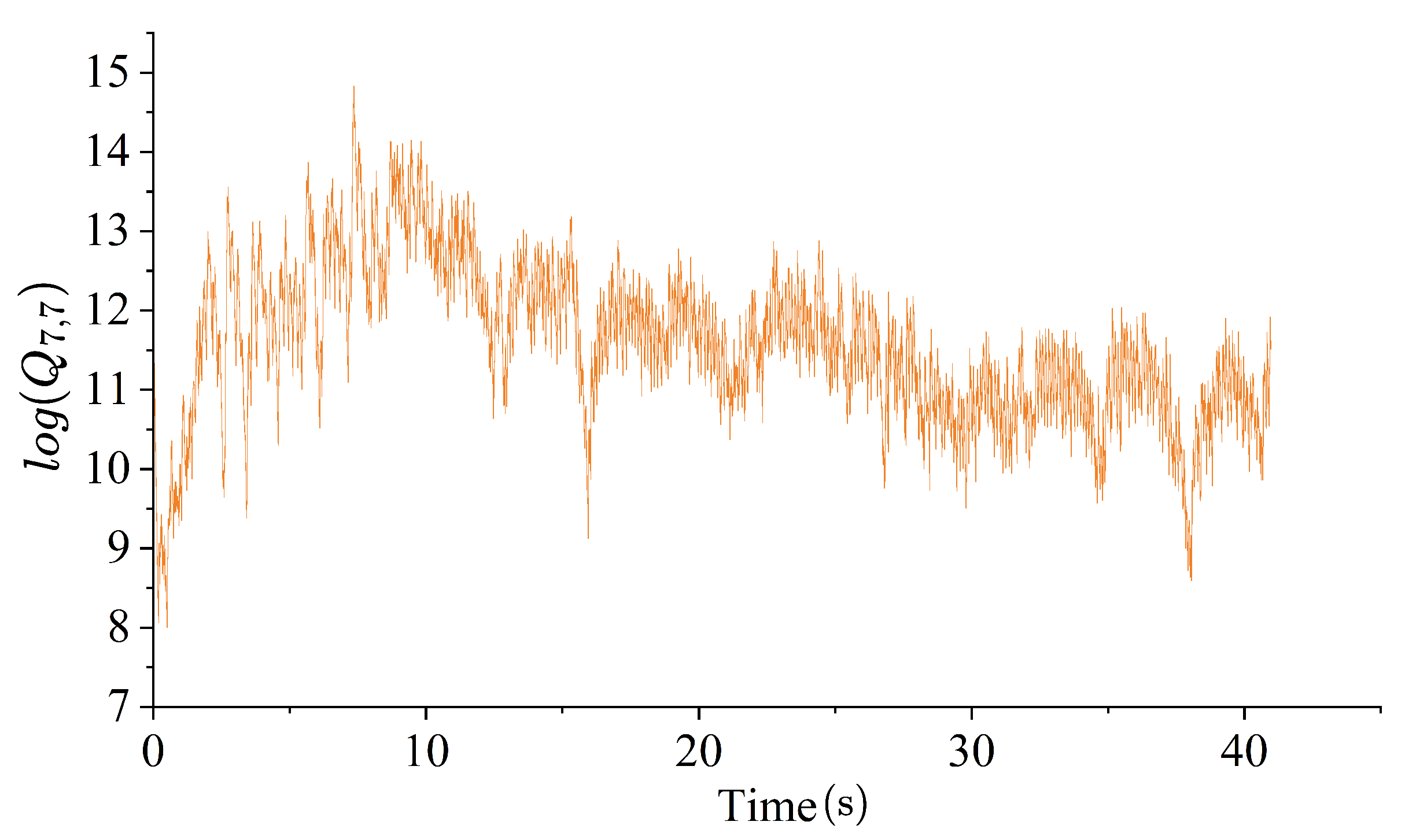
Figure 4 shows the time evolution of $Q_{77}$ (in log form) during tuning, reporting that it fluctuates around a magnitude of ${10}^{11}$ ${(\mathrm{N}/\mathrm{m})}^2$. Despite the true stiffness being $1.4\times {10}^9$ N/m, and the expectation that the process noise covariance of stiffness would have a high magnitude, it remains challenging to tune $Q_{77}$ to a higher degree of accuracy.

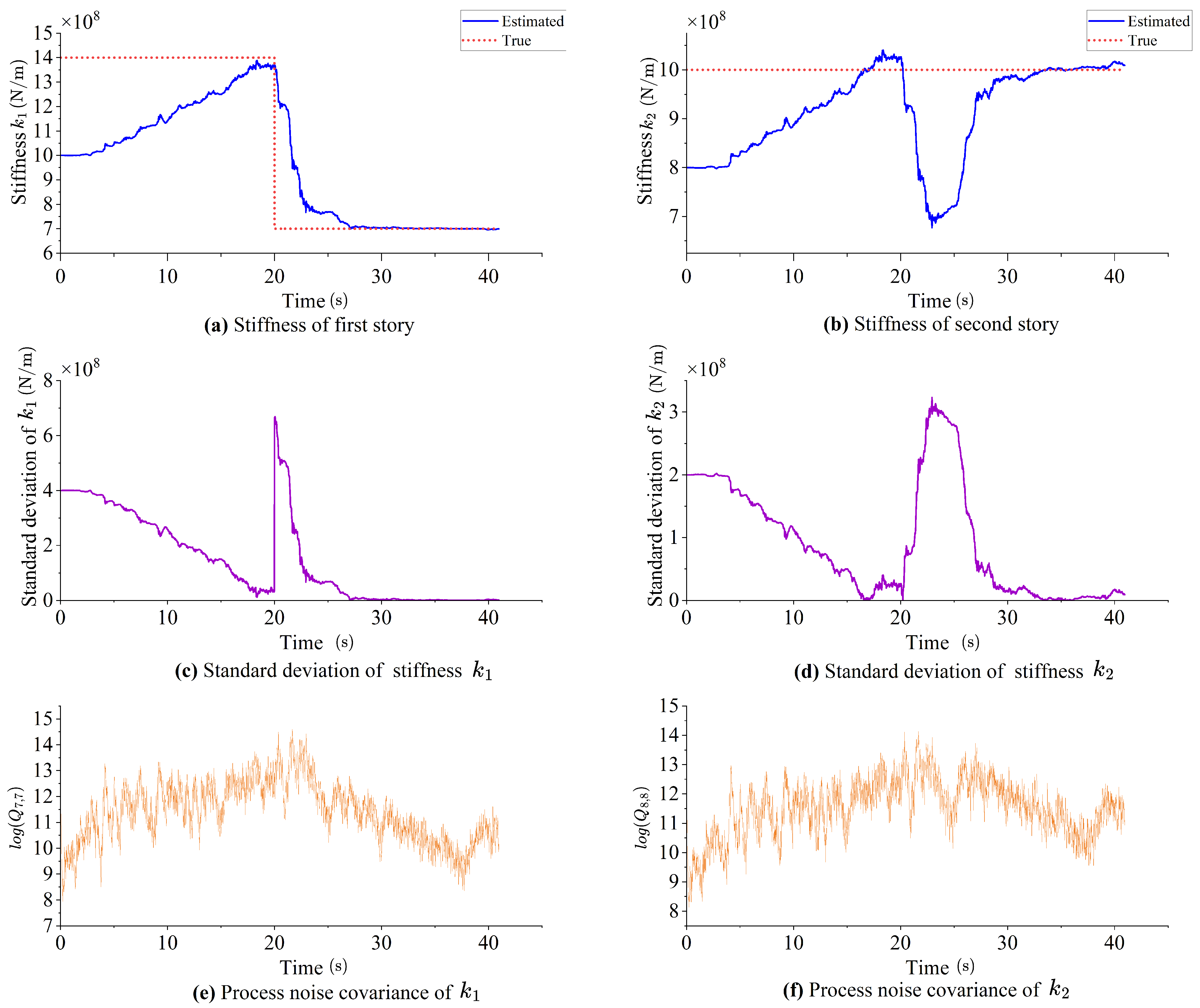
3.2. Scenario 2: Multiple Stiffness Estimation

In this case, the shear building is assumed to feature different interstory stiffness values so that $k_1=1.4\times {10}^9$ N/m and $k_2=1\times {10}^9$ N/m. The initial guesses of stiffness are chosen to be significantly different from the true values: $k_{1,0}=1\times {10}^9$ N/m and $k_{2,0}=1.6\times {10}^9$ N/m. As shown in Figure 5, although it takes about 30 s for $k_1$ and $k_2$ to converge to the true values, the final estimations exhibit high accuracy and stability. This demonstrates that the AEKF can effectively update the structural model even when multiple structural parameters are unknown.

3.3. Scenario 3: Multiple Stiffness Estimation in the Presence of a Damage Event

To testify that the AEKF can operate under more complex conditions and detect damage, the stiffness $k_1$ of Scenario 2 is reduced to half at 20 s, so that a damage is allowed to occur on the first interstory. As shown in Figure 6, the stiffness estimation reacts quickly to the sudden change in $k_1$, and it takes approximately 10 s for the estimations of both $k_1$ and $k_2$ to converge again to the correct values.

These further results indicate that, as an online SHM method, the adaptive EKF can detect structural changes and respond promptly by updating the structural parameters. Results of the same quality, even if not shown here for brevity, cannot be obtained with the EKF.

4. Discussion

The Adaptive Extended Kalman Filter has been proposed to avoid issues related to the setting of the process noise covariance matrix. By automatically tuning all its entries thanks to the innovation sequence, a significantly improvement of the accuracy of state and stiffness estimations has been achieved. The filter has also demonstrated a good performance in multi-parameter estimation, allowing for the updating of structural parameters related to the stiffness, possibly mimicking the presence of damage even in the absence of direct measurements.

Future research will focus on developing methods to improve the stability and accuracy of the estimation of the process noise covariance. Moreover, a procedure to set the most efficient forgetting factor $\alpha$ will be proposed with the aid of machine learning algorithms. Ultimately, this online SHM method will be enhanced using high-performance computing to achieve real-time SHM on high-dimensional structures.

References

- Straits Research: Structural Health Monitoring Market Size Is Projected to reach USD 7.59 Billion by 2030. 2022. Available online: https://www.globenewswire.com/en/news-release/2022/08/02/2490603/0/en/Structural-Health-Monitoring-Market-Size-is-projected-to-reach-USD-7-59-Billion-by-2030-growing-at-a-CAGR-of-14-7-Straits-Research.html (accessed on 20 August 2024).
- Kalman, R.E. A new approach to linear filtering and prediction problems. J. Basic Eng. 1960, 82, 35–45. [Google Scholar] [CrossRef]
- Schmidt, S.F. Application of State-Space Methods to Navigation Problems. Adv. Control. Syst. 1966, 3, 293–340. [Google Scholar] [CrossRef]
- Mehra, R. Approaches to adaptive filtering. IEEE Trans. Autom. Control 1972, 17, 693–698. [Google Scholar] [CrossRef]
- Rosafalco, L.; Azam, S.E.; Mariani, S.; Corigliano, A. System Identification via Unscented Kalman Filtering and Model Class Selection. ASCE-ASME J. Risk Uncertain. Eng. Syst. Part A Civ. Eng. 2024, 10, 04023063. [Google Scholar] [CrossRef]
- Bathe, K.J. Finite Element Method. In Wiley Encyclopedia of Computer Science and Engineering; John Wiley & Sons, Ltd.: Hoboken, NJ, USA, 2008; pp. 1–12. [Google Scholar] [CrossRef]
- Torzoni, M.; Manzoni, A.; Mariani, S. Structural health monitoring of civil structures: A diagnostic framework powered by deep metric learning. Comput. Struct. 2022, 271, 106858. [Google Scholar] [CrossRef]
- Rosafalco, L.; Torzoni, M.; Manzoni, A.; Mariani, S.; Corigliano, A. Online structural health monitoring by model order reduction and deep learning algorithms. Comput. Struct. 2021, 255, 106604. [Google Scholar] [CrossRef]
- Kalman, R.E.; Bucy, R.S. New results in linear filtering and prediction theory. ASME J. Basic Eng. 1961, 83, 95–108. [Google Scholar] [CrossRef]
- Ljung, L. The Extended Kalman Filter as a Parameter Estimator for Linear Systems; Linköping University: Linköping, Sweden, 1977. [Google Scholar]
- Ljung, L. System identification. In Signal Analysis and Prediction; Springer: Berlin/Heidelberg, Germany, 1998; pp. 163–173. [Google Scholar]
- Nelson, A.T. Nonlinear Estimation and Modeling of Noisy Time Series by Dual Kalman Filtering Methods; Oregon Graduate Institute of Science and Technology: Hillsboro, OR, USA, 2000. [Google Scholar]
- Bittanti, S.; Maier, G.; Nappi, A. Inverse problems in structural plasticity: A Kalman filter approach. In Plasticity Today: Modelling, Methods and Applications; Sawczuck, A., Bianchi, G., Eds.; Elsevier: Amsterdam, The Netherlands, 1984; pp. 311–329. [Google Scholar]
- Bolzon, G.; Fedele, R.; Maier, G. Parameter identification of a cohesive crack model by Kalman filter. Comput. Methods Appl. Mech. Eng. 2002, 191, 2847–2871. [Google Scholar] [CrossRef]
- Catlin, D.E. Estimation, Control, and the Discrete Kalman Filter; Springer Science & Business Media: Berlin/Heidelberg, Germany, 2012; Volume 71. [Google Scholar]
- Wan, E.A.; Nelson, A.T. Dual extended Kalman filter methods. In Kalman Filtering and Neural Networks; Wiley-Interscience: Hoboken, NJ, USA, 2001; pp. 123–173. [Google Scholar]
- Hoshiya, M.; Saito, E. Structural identification by extended Kalman filter. J. Eng. Mech. 1984, 110, 1757–1770. [Google Scholar] [CrossRef]
- Song, M.; Astroza, R.; Ebrahimian, H.; Moaveni, B.; Papadimitriou, C. Adaptive Kalman filters for nonlinear finite element model updating. Mech. Syst. Signal Process. 2020, 143, 106837. [Google Scholar] [CrossRef]
- Mariani, S.; Corigliano, A. Impact induced composite delamination: State and parameter identification via joint and dual extended Kalman filters. Comput. Methods Appl. Mech. Eng. 2005, 194, 5242–5272. [Google Scholar] [CrossRef]
- Akhlaghi, S.; Zhou, N.; Huang, Z. Adaptive adjustment of noise covariance in Kalman filter for dynamic state estimation. In Proceedings of the 2017 IEEE Power & Energy Society General Meeting, Chicago, IL, USA, 16–20 July 2017; pp. 1–5. [Google Scholar] [CrossRef]
- Eftekhar Azam, S.; Mariani, S. Online damage detection in structural systems via dynamic inverse analysis: A recursive Bayesian approach. Eng. Struct. 2018, 159, 28–45. [Google Scholar] [CrossRef]
- Hughes, T.J.R. The Finite Element Method; Dover Publication: New York, NY, USA, 2007. [Google Scholar]