Abstract
In today’s engineering applications, model-based fault diagnosis methods are used, especially to reduce existing costs. This study is a continuation of the previous works conducted by the authors, and it fundamentally includes model-based fault diagnosis methods. Within the scope of this study, the residual value structure of tire pressure is integrated into the previously created Bayesian network structure, aiming to achieve a more accurate detection of the fault present in the tire. The updated method is first modeled and tested in the Matlab/Simulink environment. Subsequently, the algorithm structure and the resolution algorithms that allow us to obtain the tire pressure values from the vehicle are updated in an ROS environment, and the designed method is verified with real vehicle tests. Here, a test scenario for the tire pressure is created, and a real vehicle test is conducted. The faults obtained during the test are also displayed on the Human–Machine Interface.
1. Introduction
Recent advancements in technology have made autonomy features an indispensable part of modern vehicles. These systems enable automotive companies to provide a safer, more comfortable, and more convenient driving experience. This transformation in the automotive industry has reached the next level with the general safety regulations (GSR) implemented by the European Union. As of July 2024, many systems such as drowsiness detection, lane keeping, emergency braking, and tire pressure monitoring have become mandatory depending on vehicle type [1]. The common feature of these systems is that they all process data from sensors on the vehicle and perform actions that will either increase driving safety and comfort or warn the driver. Any malfunction of the sensors can prevent these systems from working as intended, and this can pose a serious safety risk. Therefore, it is very important to be able to detect faults in sensors and determine whether the problem is caused by sensor reading or a physical reason.
As a result of innovative fault detection and diagnosis methods [2,3,4,5], the safety and reliability of technical processes have improved. It is possible to classify fault detection methods under three main headings: model-based methods, knowledge-based methods, and data-driven methods [6]. Model-based fault detection is a method that effectively detects faults in complex systems [7]. This method detects deviations from normal operation using mathematical models of systems and determines the causes of faults. Reliable results are obtained by comparing the values calculated using analytical models with the measured values [8]. Model-based fault detection is advantageous in terms of cost, since it does not bring additional cost and weight. However, correct modeling and regular updates are of great importance.
Fault trees and signal-based methods are frequently used among knowledge-based methods. Since these methods do not require mathematical modeling, the complexity and uncertainty brought by system modeling are not present [9]. In the fault tree method, the user is asked a series of questions expressing possible fault symptoms, and the cause of the fault is tried to be determined according to the answers given by the user to these questions [10]. Although fault trees are practical and user-friendly, they have some important disadvantages. For example, when there is uncertainty about a particular cause of failure, the model does not address it. In addition, the fixed structure of the tree prevents the inclusion of expertise or previous knowledge in the diagnosis process and may have difficulty in identifying faults that show more than one symptom [11]. It is difficult to obtain a set of rules that will detect a possible fault for complex systems, and since fault detection is directly based on this set of rules, the system cannot detect problems if fault information is not collected and a lack of adaptation to unknown problems occurs [12]. Signal-based fault detection systems are also an effective method used to detect faults in complex systems [13]. This method detects faults by analyzing the measured output signals of the system. Faults in the system are usually associated with changes in the characteristics of the measured signals and are detected through these changes. In [14], the authors used model-based and signal-based approaches to perform fault diagnosis on an induction motor, and concluded that although the model-based approach is more difficult to implement than the signal-based approach due to the complexity of the models used, it performs better.
Data-driven methods approach fault detection as a pattern recognition problem. Based on data processing, sample data are collected and trained to obtain a classifier, and then the data are matched according to the classification rules [15]. Techniques such as artificial neural networks and deep learning have received widespread usage in these methods in recent years.
In this study, a model-based fault detection method was developed by adding four new residual values of wheel pressure to the structure of the Bayesian network developed by the authors in [16,17]. As a result of this addition, a significant improvement was observed in the system’s ability to detect faults occurring in the wheels. In the remainder of this study, the fault detection plan and the integration of the new residual values into the existing Bayesian network is explained. Then, the results of the real-time tests performed on the test vehicle are shared and evaluated.
2. Fault Diagnosis Structure
2.1. Sensors
In the model [16,17] that was previously developed by the authors, there are three residuals for the yaw rate, two residuals for the tire slip, and one residual for the steering wheel angle, which gives a total of six residuals. In this work, compared to the previous model, four more residuals are added that are based on the tire pressure. Including these pressure residuals, the total number of residuals is increased to ten. Table 1 illustrates the parameters that are measured by the sensors.

Table 1.
The definition of the parameters that are measured by the sensors.
2.2. Calculatıon of Tire Pressure Residuals
In this work, ten residuals are obtained from six different models for the purpose of fault diagnosis. The details of these models are provided in [16,17]. Three of these models are used for calculating the yaw rate. Two of these models are utilized for calculating the wheel slip, and the last model is utilized for calculating the steering wheel angle. The details of these six models and calculation of the related residuals are provided in [16,17]. In this work, the remaining residuals related to the wheel pressure are explained. The details of the reference values of each wheel is explained in the Test Scenario section. The difference between these reference values and the pressure values measured using the tire pressure sensors gives total of four residuals:
In Equation (1), shows the reference pressure value of each tire, whereas shows the pressure value measured using the tire pressure sensor. The difference between these two values give the seventh, eighth, ninth, and the tenth residuals.
2.3. Fault Diagnosis Algorithm
As explained in [1], the three residuals related to the yaw rate are obtained by taking the difference between the yaw rate value calculated using the model and the yaw rate value measured using the yaw rate sensor. Besides that, two more residuals are obtained by taking the difference between the wheel slip value calculated from the wheel force relation and the wheel slip value obtained by using the left and right wheel speed values. The sixth residual is obtained by taking the difference between the value calculated by the steering wheel angle and the value measured using the steering wheel angle. Finally, the pressure residuals are obtained for each wheel using Equation (1). Hence, four more residuals are obtained. Besides these residuals, there are total of ten faults where four of them are physical and the other six faults are related to the sensors. The faults and their descriptions are given in Table 2.
Table 2.
Faults and their descriptions.
The Bayes Network that relates the faults is shown in Table 2, and the calculated residuals is illustrated in Figure 1.
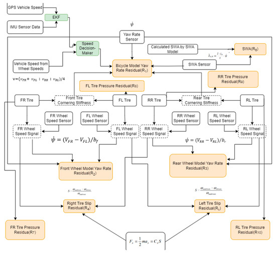
Figure 1.
Fault diagnosis algorithm scheme.
2.4. Dynamic Bayesian Network
In this work, the fault probabilities are calculated using a Bayesian Network. According to this structure, in the case of a residual becoming activated, the fault probabilities that are related to this residual are dynamically updated. In Figure 1, it is observed that each residual is related to a combination of different faults. The technical details of the algorithm that is composed of six residuals (which does not include the residuals related to the pressure values) is given in [16]. Table 3 illustrates the specific faults that are being activated in the case-specific combination of residuals that are being activated.
Table 3.
The faults and related residuals that are activated.
Different to the previous work of the authors [1], for the activation of , , , and faults, the , , , and residuals also need to exceed the determined thresholds, respectively. This can be easily deduced from Equation (1).
2.5. ROS Structure
The general logic of ROS structure is explained in [17]. In this work, the details related to the new updates are explained.
Wheel pressure data are required for updating the fault diagnosis structure of the algorithm. For this reason, the ROS node structure in [17] is updated. Wheel pressure is obtained using a DBC (CAN Database) file that belongs to the vehicle. In that sense, some tests have been performed on the vehicle to determine with which CAN message the wheel pressure is obtained. The data are recorded in cases where the wheel pressure is lowered, and by investigating the data, the CAN message used to obtain the pressure data are detected. Figure 2 illustrates the CAN message list that belongs to the vehicle.
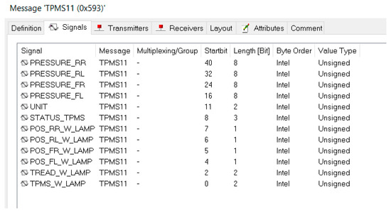
Figure 2.
The vehicle’s CAN message list.
After the CAN ID is detected, the length of the data is investigated and the number of bits in the data is calculated. Later, CAN ID that belongs to the wheel pressure is added inside the code where the data are parsed according to the length and unit of the data (Figure 3). Because the unit of the pressure data is in bar, the data are multiplied by a coefficient to convert their units to PSI.
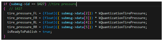
Figure 3.
Data parsing function for the tire pressure.
The residual structure is obtained by comparing the pressure data and the reference pressure value of the vehicle. The ROS package is updated by adding residuals into a Bayesian Network structure to obtain the fault probabilities. In the next section, the results obtained from the real vehicle test are discussed.
3. Test Scenario
The tests of the fault detection algorithm integrated into ROS are carried out using real vehicle data. The test scenario is applied to a real vehicle, and the fault detection is observed online. When determining the reference and threshold values for the test scenario, the tire pressure values of the Kia Niro vehicle are used. Accordingly, reference values of 2.3 PSI for the front tires and 2.1 PSI for the rear tires are established. Additionally, if the residual values exceeded 0.4 PSI, it is observed that a fault occurred in the vehicle’s tire. These reference and threshold values are also taken as the basis during the test.
3.1. Test Scenario
Right Front Tire Pressure Fault Scenario
Before the test scenario is conducted, the pressure of the vehicle’s front-right tire is lowered. In this way, tire pressure value to drop below the reference, causing the residual value of the tire pressure to exceed the threshold value. The pressure values of the front right tire, along with those of the other tires, are presented in Table 4.
Table 4.
Tire pressure and tire faults.
During the test, the computer is connected to the vehicle, and the written ROS node is executed using the vehicle’s fault detection algorithm with the tire pressures specified in Table 4. The output of the Bayesian network structure, shown in Figure 4, indicated that the fault is statistically attributed to the front-right tire. A flag value of 1 is assigned to the point with the highest fault probability (with the condition that it exceeds 70%), marking that value as faulty. As the front-right tire exhibited the highest fault probability during this test, it is marked as faulty with a value of 1, as detailed in Table 4.
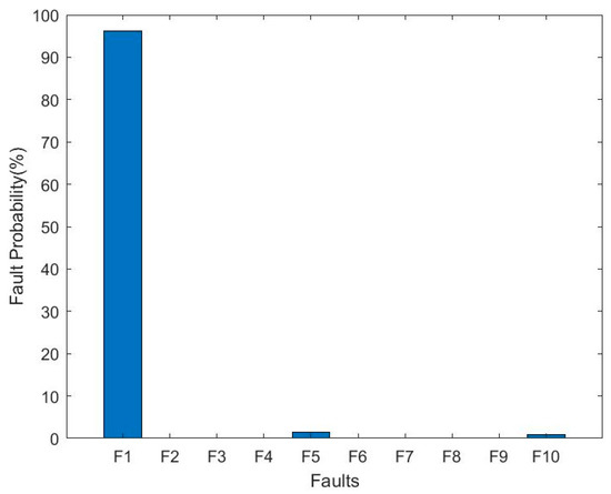
Figure 4.
Fault probability values.
In addition, this faulty value is shown on the HMI, as in Figure 5. In this way, the user can easily track which sensor or actuator is faulty at that moment from the HMI.
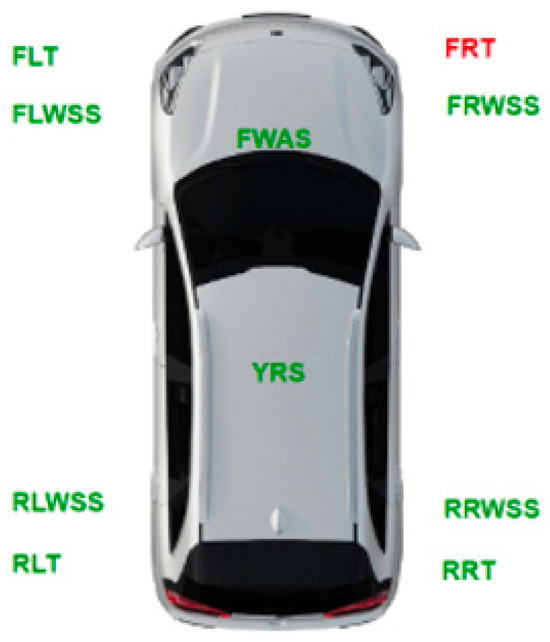
Figure 5.
Displaying the fault result on the HMI screen.
4. Results
This study builds on previous research [16,17] by enhancing the fault detection capabilities of existing models. Four new residual structures, specifically related to wheel pressures, were integrated to improve the detection of physical wheel faults with greater statistical accuracy. The mathematical models developed were first simulated using Matlab/Simulink and then in ROS, followed by real vehicle tests to validate the simulation results. The tests confirmed that the proposed algorithm effectively detects faults with high statistical reliability, successfully displaying the detected faults on the user interface and providing timely feedback to the user.
Author Contributions
Conceptualization, T.B., M.G. and B.K.; methodology, T.B. and M.G.; software, T.B., M.G. and B.K.; writing—original draft preparation, T.B., M.G. and B.K.; validation, T.B., M.G. and B.K.; investigation, T.B., M.G. and B.K.; supervision, T.B. All authors have read and agreed to the published version of the manuscript.
Funding
This research received no external funding.
Institutional Review Board Statement
Not applicable.
Informed Consent Statement
Not applicable.
Data Availability Statement
Data sharing does not apply to this paper.
Conflicts of Interest
The authors declare no conflicts of interest.
References
- European Commission. New Rules to Improve Road Safety and Enable Fully Driverless Vehicles in the EU; European Commission: Brussels, Belgium, 2022; Available online: https://ec.europa.eu/commission/presscorner/detail/en/ip_22_4312 (accessed on 18 July 2024).
- Ko, C.; Fox, D. GP-BayesFilters: Bayesian filtering using Gaussian process prediction and observation models. Int. J. Robot. Res. 2009, 28, 1524–1547. [Google Scholar] [CrossRef]
- Wang, Z.; Gao, Z.; Ding, S.X. A survey of model-based fault detection and diagnosis methods. Acta Autom. Sin. 2012, 38, 823–839. [Google Scholar]
- Chen, J.; Patton, R.J. Robust Model-Based Fault Diagnosis for Dynamic Systems; Kluwer Academic Publishers: New York, NY, USA, 1999. [Google Scholar]
- Raghuraman, S.; Mahadevan, S. Fault detection and diagnosis using dynamic Bayesian networks and system identification. J. Process Control 2010, 20, 604–616. [Google Scholar]
- Wu, H.; Zhao, J. Deep convolutional neural network model based chemicalprocess fault diagnosis. Comput. Chem. Eng. 2018, 115, 185–197. [Google Scholar] [CrossRef]
- Ding, S.X. Model-Based Fault Diagnosis Techniques: Design Schemes, Algorithms, and Tools; Springer: Berlin, Germany, 2008. [Google Scholar]
- Marzat, J.; Lahanier, H.P.; Damongeot, F.; Walter, E. Model-based fault diagnosis for aerospace systems: A survey. Proc. Inst. Mech. Eng. Part G J. Aerosp. Eng. 2011, 226, 1329–1360. [Google Scholar] [CrossRef]
- Xu, Z.; Liang, M.; Chen, X.; Sun, Y. A survey of data-driven approaches for condition monitoring and fault diagnosis of electrical machines. IEEE Trans. Ind. Electron. 2017, 65, 3990–4001. [Google Scholar]
- Ji, L.; Zhang, Y.; Yan, R.; Song, Y. Fault diagnosis of power transformers based on fault tree and fault tree-analytic hierarchy process. Electr. Power Syst. Res. 2019, 174, 105822. [Google Scholar]
- Huang, Y.; McMurran, R.; Dhadyalla, G.; Peter Jones, R. Probability based vehicle fault diagnosis: Bayesian network method. J. Intell. Manuf. 2008, 19, 301–311. [Google Scholar] [CrossRef]
- Li, D.; Wang, Y.; Wang, J.; Wang, C.; Duan, Y. Recent advances in sensor fault diagnosis: A review. Sens. Actuators A Phys. 2020, 309, 111990. [Google Scholar] [CrossRef]
- Huang, B.; Zhu, Q.; Zhang, D.; Li, X. A survey of signal processing techniques for rotating machinery fault diagnosis. Measurement 2019, 136, 597–619. [Google Scholar]
- Harihara, P.P.; Kim, K.; Parlos, A.G. Signal-based versus model-based fault diagnosis-a trade-off in complexity and performance. In Proceedings of the 4th IEEE International Symposium on Diagnostics for Electric Machines, Power Electronics and Drives, SDEMPED 2003, Atlanta, GA, USA, 24–26 August 2023; pp. 277–282. [Google Scholar]
- Gao, Z.; Cecati, C.; Ding, S.X. A survey of fault diagnosis and fault-tolerant techniques part II: Fault diagnosis with knowledge-based and Hybrid/Active approaches. IEEE Trans. Ind. Electron. 2015, 62, 3757–3767. [Google Scholar] [CrossRef]
- Bodrumlu, T.; Gözüm, M.M.; Kavak, B. Enhanced Fault Detection of Vehicle Lateral Dynamics Using a Dynamically Adjustable Bayesian Network Structure and Extended Kalman Filter. In ASME International Mechanical Engineering Congress and Exposition; American Society of Mechanical Engineers: Colombus, OH, USA, 2023; p. V009T14A024. [Google Scholar]
- Yalcin, M.F.; Bodrumlu, T.; Gozum, M.M.; Ates, E. Dinamik Bayes Ağ Yapısı ve Genişletilmiş Kalman Filtresi Kullanılarak Gerçek Zamanlı ROS Uygulaması ile Otonom Bir Araçtaki Yanal Dinamiklerdeki Arıza Tespitinin Gerçeklenmesi, 24. Otomatik Kontrol Ulus. Toplantısı 2023, 408–413. Available online: https://tok2023.itu.edu.tr/docs/librariesprovider68/bildiriler/tok2023-bildiri-kitabi.pdf?sfvrsn=16ceecde_0 (accessed on 18 July 2024).
Disclaimer/Publisher’s Note: The statements, opinions and data contained in all publications are solely those of the individual author(s) and contributor(s) and not of MDPI and/or the editor(s). MDPI and/or the editor(s) disclaim responsibility for any injury to people or property resulting from any ideas, methods, instructions or products referred to in the content. |
© 2024 by the authors. Licensee MDPI, Basel, Switzerland. This article is an open access article distributed under the terms and conditions of the Creative Commons Attribution (CC BY) license (https://creativecommons.org/licenses/by/4.0/).