Transformation of Guided Ultrasonic Wave Signals from Air Coupled to Surface Bounded Measurement Systems with Machine Learning Algorithms for Training Data Augmentation ^†

Abstract

Guided ultrasonic wave (GUW) analysis is a well-investigated method for structural health monitoring (SHM) applications. For plate-like structures, the pitch-catch technique is a popular choice since it offers the possibility to investigate a large area with a small number of sensors. This method requires a large amount of data to be analyzed to detect and localize damage, with the consequence that, besides the presence of damage, environmental influences like temperature and load will also change the GUW signals. In addition, the location, size, and type of the damage will result in different changes in the GUW signals. Data-driven methods require sufficient data and therefore require data augmentation. In order to get closer to this goal, this study aims to demonstrate the conversion of GUW signals measured with an air-coupled measurement system (ACMS) into signals measured with piezoelectric wafer active sensors (PWAS). This would allow the fast measurement of GUW data with ACMS at different positions of a plate-like specimen and translate it to a surface-bonded PWAS signal without the time-consuming process of transducer mounting. In this study, it is assumed that the measurement methods are not independent of each other when they are measured at the same position. To obtain the transform function from ACMS to PWAS, GUW signals were measured both with ACMS and PWAS for different positions of artificial damage. Since both signal classes are physically dependent, it should be possible to determine the transform function with machine learning (ML) methods. As input, the ACMS time-dependent signal or signal features are used, while the PWAS signals serve as labels for the training process. We are evaluating different ML-based transform model architectures with respect to their suitability for signal or signal feature transformation, e.g., ANN, CNN, and LSTM-based networks, with a particular focus on autoencoders.

1. Introduction

The aim of structural health monitoring (SHM) is to derive information about a structural state [1] using suitable measuring methods. For plate-like structures, guided ultrasonic waves (GUW) [2] are a common tool for SHM systems [3]. Damages and defects will change the GUW signal by adding damage-related signal features. GUW-based measuring techniques offer the advantage of monitoring a large area with a relatively small number of transducers [4,5]. The disadvantage of GUW signals is their sensitivity to environmental states, like temperature [6,7], too. This makes the interpretation of changes in GUW signals challenging, so in recent years, machine learning (ML) approaches have been used for GUW-based SHM [8]. Since ML methods rely on a sufficient amount of training data with sufficient parameter variance, it is often very time-consuming to measure GUW signals at different temperatures and under different damage states. To overcome this problem, simulated GUW data can be used for ML training [9,10,11], but this suffers from a reality gap and accuracy loss. Another approach is the application of data augmentation; for example, in [12], an augmentation approach was proposed where GUW signal features, like the signal maximum, could be generated over a broad temperature range. The generation of aggregate variables from signals is a limiting factor, e.g., the approach from [12] can generate quite accurate aggregate data, but a reconstruction of the original time-resolved signal is not possible.

In this work, a new approach is developed to increase the amount of GUW data. We propose signal transformation generative models trained from experimental data. It is based on the conversion of GUW signals measured with a spatially resolved air-coupled measurement system (ACMS) into signals measured with piezoelectric wafer active sensors (PWAS). This allows the fast measurement of GUW data with ACMS at different positions of a specimen with fine spatial resolution and transforms it to a surface-bonded PWAS signal. It is assumed that the in-plane and out-plane displacements of a GUW are not independent of each other, so that the different measurement approaches can be converted into each other, regardless of the sensitivity of the individual measuring systems to the different displacement fields. To achieve this, in the present work, different ML-based transform model architectures are used and investigated, e.g., artificial neural networks (ANN), convolutional neural networks (CNN), recurrent long short-term memory networks (LSTM), and autoencoders (AE) with ANN and CNN architectures. Because time-resolved and phase-sensitive sensor signals are transformed, the generative models must satisfy some constraints: phase, amplitude, and frequency invariance. Some of the evaluated models will not satisfy all constraints and will be considered here only for a proof-of-concept exploration.

It is shown that, in general, a transformation between ACMS- and PWAS-signals is possible and that various ML architectures are able to perform this task. But there are also systematic problems, e.g., all ML architectures deliver poor results for some specific ACMS signals, which have to be addressed in future work to make this approach reliable to use.

2. Methods and Experiments

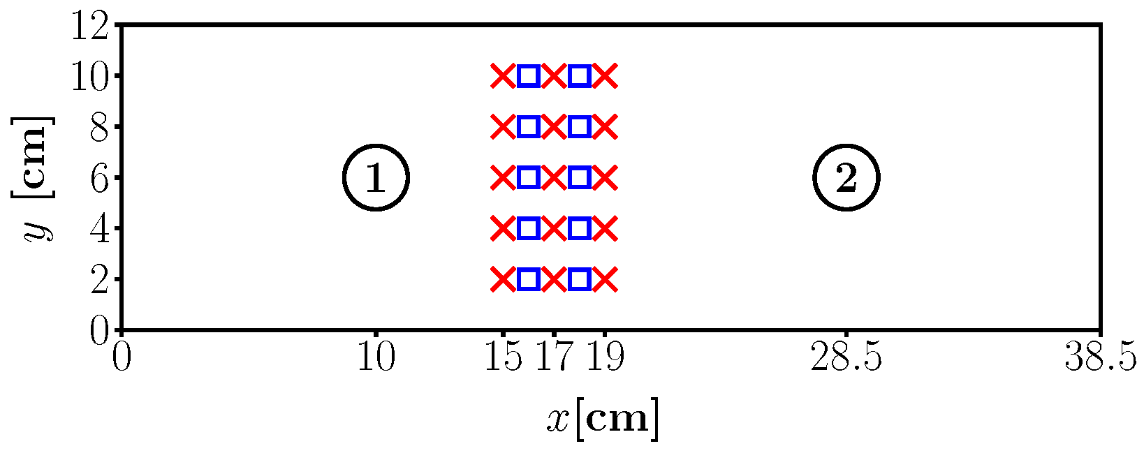
2.1. Experimental Setup

The GUW were measured on a Glass Laminate Aluminum Reinforced Epoxy (GLARE) plate with a GLARE3-3/2 standard layup [13]. The dimensions of the plate are $38.5\times 12\times 0.23$ cm. At the surface of the plate, two PWAS transducers (DuraAct from PI Ceramics) were adhesively bonded using an epoxy resin film that was cured in an oven while surrounded by a vacuum bag. This way, a highly homogeneous resin film thickness between the transducers and the surface could be achieved. For the GUW measurements, two magnets with a diameter of $1$ cm were used as local disturbances (artificial damage). The magnets were positioned at different locations on the plate. A sketch of the plate with the transducer and magnet positions is shown in Figure 1.

For every magnet position and the case where no magnets were on the plate, two PWAS GUW measurements (PM) were performed; one was PWAS 1 acting as an actuator and PWAS 2 as a sensor, and vice versa. The corresponding air-coupled GUW measurements (AM) were performed with a MEMS-1-microphone (SPU0410LR5H-QB) at the position of the sensor, but on the other side of the plate, to ensure that the surface of the plate was scanned and not the surface of the PWAS. Since the PWAS measures the GUW over an area and not at a single point, the MEMS scanned the surface at the sensor position with the help of a CNC machine. The scanning points with respect to the center of the PWAS sensor are shown in Figure 2.

The pitch signal is a five-cycle Hanning windowed sine signal with a center frequency of $25$ kHz. This low frequency was chosen since, at this frequency, the MEMS microphone (SPU0410LR5H-QB, Knowles Electronics, LLC., Itasca, IL, USA) is most sensitive. The frequency response of the MEMS microphone is about 100–80 kHz [14]. To suppress environmental noise, a low-pass filter with a roll-off frequency of about 5 kHz was used in the pre-amplifier with a gain of 50. Based on the technical specifications, we assume that the frequency spectrum of the captured signals is 5–100 kHz (with an additional high-pass filter). The high frequencies of the signal spectrum could have an impact on the signal transformation process and its accuracy.

2.2. Data Preprocessing

Before the GUW data were used for model training and testing, minor preprocessing was performed. At first, the data were normalized with respect to the signal maximum. As mentioned before, the PWAS measures the GUW over its whole area; the MEMS microphone, on the other hand, measures the GUW over a much smaller area, so that here an almost point-wise measurement is performed. Due to that, a direct transformation of a single a.m. to a p.m. signal should come with difficulties, since this would be a transformation of a point to an area measurement. This also leads to the fact that for 9 a.m., just one PM exists (see Figure 2), which could lead to problems during model training, since the a.m. differ in phase and amplitude while the PM stays the same. To investigate this, two data sets were created: one where the single AM is directly transmitted to p.m., so that there are still 9 a.m. for one PM, and a second data set where the 9 a.m. of a sensor scan are averaged, so that just one average signal exists per p.m. The first data set is called single signal data (SSD), while the second is called average signal data (ASD). In the next step, Gaussian noise was added to the data to increase the number of training and test data, where the noise could vary by five percent from the signal value.

2.3. Machine Learning Models

For the experimental investigations, we used different ML architectures trained and evaluated with the same data. This includes common feed-forward ANN, CNN, recurrent and state-based LSTM, and AE with ANN and CNN architectures. The models must satisfy signal constraints, mainly phase, amplitude, and frequency invariance, to ensure broad coverage of the parameter space and signal features. Due to the static connections of ANN nodes with the input data, ANN architecture will not satisfy any of the three constraints in a general way but can represent a signal subspace, as shown in the experimental evaluation. For phase and partially frequency invariance, a moving window approach is required, as provided by the CNN and implicitly by the LSTM architectures (as well as the appropriate AE architectures).

All models are implemented with TensorFlow and use the Adam optimizer. In this work, no hyperparameter tuning was performed so that the TensorFlow default values: training rate $\alpha =0.001$, momentum ${\beta }_1=0.9$, and ${\beta }_2=0.99$ were used. For every data set, a whole AM time signal is used as input, so that signal is an entire input vector, and the number of input nodes corresponds to the number of data points in the time signal. The node number of the output layer of each model corresponds to the number of data points in the PM time signal, commonly equal to the input vector size. In

Table 1. Architecture of the different models used in this study.

Model	Layer Class	Parameters	Activation Function
ANN	Input	N: 6249; OS: [6249]; P: 0	-
	Dense	N: 6249; OS: [6249]; P: 39056250	tanh
	Dense	N: 6249; OS: [6249]; P: 39056250	linear
CNN	Input	N: 6249; OS: [6249]; P: 0	-
	Conv1D	K: 16; KS: 12; S: 1; PC: valid; OS: [6227, 16]; P: 208	tanh
	Conv1D	K: 16; KS: 12; S: 1; PC: valid; OS: [6227, 16]; P: 3088	tanh
	Flatten	OS: [99632]; P: 0	-
	Dense	N: 6249; OS: [6249]; P: 622606617	tanh
LSTM	Input	N: 6249; OS: [6249]; P: 0	-
	LSTM	N: 3; OS: [6249, 3]; P: 60	tanh
	LSTM	N: 3; OS: [6249, 3]; P: 84	tanh
	LSTM	N: 3; OS: [6249, 3]; P: 84	tanh
	LSTM	N: 3; OS: [6249, 3]; P: 84	tanh
	LSTM	N: 3; OS: [6249, 3]; P: 84	tanh
	LSTM	N: 1; OS: [6249, 1]; P: 20	tanh
	TimeDistributed(Dense)	N: 1; OS: [6249, 1]; P: 2	linear
ANN AE	Input	N: 6249; OS: [6249]; P: 0	-
	Dense	N: 124; OS: [124]; P: 775000	tanh
	Dense	N: 64; OS: [64]; P: 7750	tanh
	Dense	N: 124; OS: [124]; P: 7812	tanh
	Dense	N: 6249; OS: [6249]; P: 781125	linear
CNN AE	Input	N: 6249; OS: [6249]; P: 0	-
	Conv1D	K: 64; KS: 4; S: 1; PC: same; OS: [6249, 64]; P: 320	tanh
	AveragePooling1D	PS: 10; S: 5; PC: same; OS: [1250, 64]; P: 0	-
	Conv1D	K: 64; KS: 4; S: 1; PC: same; OS: [1250, 64]; P: 16448	tanh
	Flatten	OS: [80000]; P: 0	-
	Dense	N: 1250; OS: [1250]; P: 100001250	tanh
	Reshape	OS: [1250, 1]; P: 0	-
	UpSampling1D	OS: [6250, 1]; P: 0	-
	Cropping1D	OS: [6249, 1]; P: 0	-
	Conv1DTranspose	K: 64; KS: 4; S: 1; PC: same; OS: [6249, 64]; P: 320	tanh
	Dense	N: 6249; OS: [6249, 1]; P: 65	linear

N: Number of Nodes; OS: Output Shape; P: Number of Learnable Parameter; K: Number of Kernels; KS: Kernel Size; S: Stride; PC: Padding Class; PS: Pool Size.

, the layer structure and activation functions of the different models are shown.

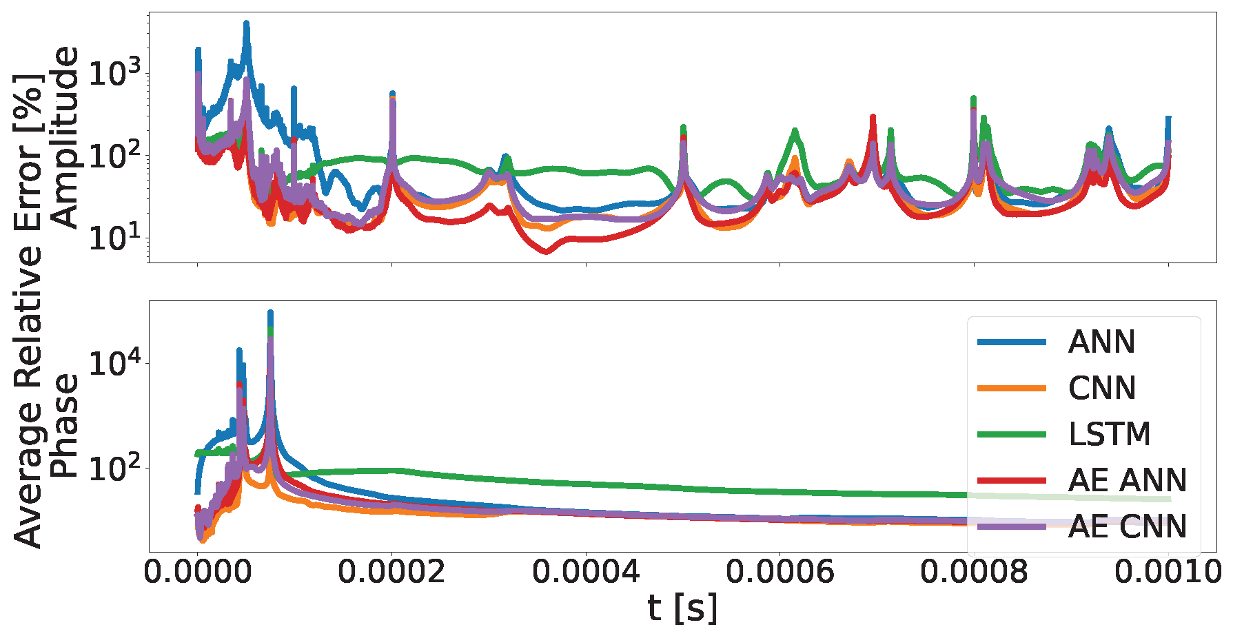
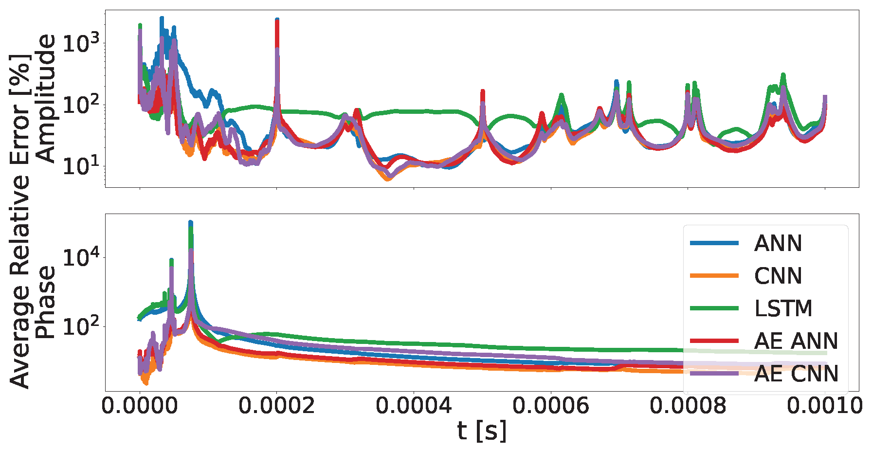
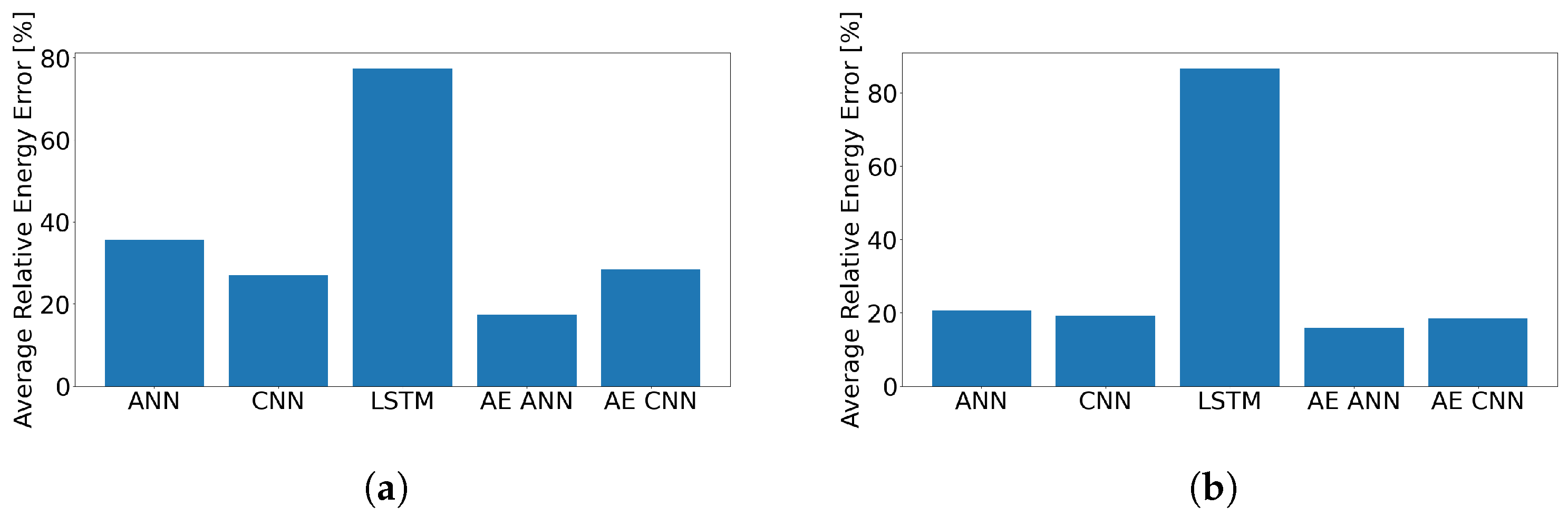
3. Results and Discussion

Since the training and test data sets were augmented with Gaussian noise, some models also generated quite noisy PM signals. Examples of this are shown in Figure 3, where the top plot displays the raw, noisy generated data. Due to this, a digital low-pass filter was applied to all outputs of the trained models; the bottom plot of Figure 3 shows the generated PM data from the top plot after the application of the filter. One can see that after the filter was applied, the quality of the signal improved significantly.

In Figure 3, it can be observed that the generated PM signal follows the pattern of the original PM signals quite well. But it was observed that for some AM inputs, the models had some problems generating a signal closely aligned with the original PM signal. In general, the generated signals follow the pattern of the original signal; however, for some AM inputs, there were significant errors in amplitude and phase. This behavior was observed for almost all models investigated, except for the LSTM models, which always had a large errors in amplitude and phase. In Figure 4, some examples are shown where the model-generated signals (except LSTM) fit quite well with the original PM signals (top plot); additionally, examples are shown where all models struggle to generate a signal that fits the original PM signal (bottom plot). One can see that all signals follow the pattern of the original PM signal, but in the bottom plot, at some parts, errors in phase and amplitude occur.

To investigate the overall performance of the models, the averaged relative error ($ARE$) of the test outputs was computed:

$$\begin{array}{c}\hfill ARE={\displaystyle \frac{100}{N}}\sum _{j=1}^N{\displaystyle \frac{|{\mathrm{F}}_j^{\mathrm{g}}-{\mathrm{F}}_j^{\mathrm{o}}|}{|{\mathrm{F}}_j^{\mathrm{o}}|}}\end{array}$$

(1)

where $F^{\mathrm{g}}$ and $F^{\mathrm{o}}$ donate a feature from the generated and original signal, respectively, while j is the index of the current signals and N the number of generated PM signals. The $ARE$ was calculated for the signal envelope and phase, where the envelope is used to investigate the difference in amplitude. The results for the models of the SSD are shown in Figure 5, while the results for the models of ASD are shown in Figure 6. It can be seen that for both data sets, the error is high at the beginning; this is expected since this is the part of the signal where no GUW is measured and consists only of noise. Due to that, this signal part will not be analyzed. Looking at Figure 5, one can see that the pattern for phase and amplitude errors is the same for all models except the LSTM model, which has the highest error of all models. The other models, on the other hand, perform almost equally for the phase and show, after the noise part of the signal, a decline in phase error and converge to a small error value of approximately nine percent (while the error of LSTM is 27 percent). For the amplitude error, these models seem to follow the same pattern, with AE ANN performing best. The peaks in the error curves can be attributed to the minima of the signal envelopes, where the slopes of the envelopes are steepest and therefore very sensitive to small differences between the signals.

Looking at Figure 6 to investigate the models of the ASD set, one can see that the errors in phase and amplitude follow almost the same pattern as the errors in Figure 5, with the LSTM model again performing poorly. In comparison to the SSD, the amplitude errors of the models are much closer to each other. Besides that, the ASD models follow the same error pattern as the SSD models.

For both data sets, the models show the smallest amplitude error in the time range where the initial wave packages occur (approx. $0.2$ to $0.5$ ms), while the error is higher in regions where the reflections of the plate edges were measured (from $0.5$ ms to the end of the signal). This is expected since the amplitudes of the initial waves are much higher than the amplitudes of the reflections. Since the relative error is computed, smaller differences between the signals have a much higher impact on the reflection signals than on the initial waves. Also, the models should learn the transform function of the initial waves more easily due to the higher amplitudes and the fact that these parts of the signal are not as influenced by interference with the reflected waves, which lead to a much more complex signal pattern. The after $0.5$ ms, increasing number of peaks in the amplitude error is a direct result of these complex signal patterns.

In the next step, the signal energy (SE) was computed:

$$\begin{array}{c}\hfill \mathrm{SE}=\sum _{t=0}^T{s}^2\left(t\right),\end{array}$$

(2)

with $s\left(t\right)$ being the value of a signal s at time t with the number of time-steps T. The SE gives the possibility to determine the signal quality with a single quantity by calculating its ARE. In Figure 7, the ARE of the SE is shown. One can see that AE ANN has the smallest error for both data sets and that the performance for ANN, CNN, AE ANN, and AE CNN is best for the ASD set. A surprising result is that the ANN performs so well with the given task, since it should not be phase invariant. Also, the bad performance of the LSTM models (80 percent SE error) is not expected. This architecture is designed to process time data with its memory and forget gates, and should therefore be best suited to learn time-dependent information and dependencies. The good performance of the CNN, AE ANN, and AE CNN, on the other hand, is not surprising, since the CNN learns time-dependent feature patterns by scanning the signal with its filters. While AE is a well-known tool to generate new pictures, and because a GUW can be considered as a 1D picture, the AE ANN should be good for the generation of new GUW signals.

What can also be observed in Figure 7 is that all models have at least an average SE error of 20 percent, which means that there are, in all models, some AM inputs for which the models could not generate a very good-fit PM signal. This could have various reasons, like a too small amount of valuable training data or the complex signal patterns due to edge reflections. In future work, the number of transducers and the size of the plate will be increased. Another reason for the errors could be a false approach in taking into account that the PWAS measures the GUW over an area while the MEMS performs point-wise measurements. It seems that the averaging of the AM improved the results in most cases, but it is not enough, so other approaches should be tested in the future.

4. Conclusions

In the present work, experiments with different ML models were performed to transform GUW signals measured with a MEMS microphone to GUW signals measured with a PWAS. It was shown that, in general, the pattern of the PWAS signal can be generated and that there are a lot of cases where the generated PWAS signals fit very well with the original signals. It is difficult to assess the quality of the transformation process. Pure statistical analysis can be misleading, and the quality of the data relies strongly on its deployment and processing. Parallel models (i.e., the entire input signal is the model input vector) perform well, but only models dynamically connecting to input data with a moving window method (e.g., CNN) can satisfy phase and partially frequency invariance, which is required for generalized and universal transformation models.

We observed that there were also some cases where, independent of the model used, the error in amplitude and phase was quite high. Also, some models, like the LSTM, failed to learn the transfer function between AM and PM measurements, which can result from the limited “memory window” of LSTM with respect to the number of time points, commonly limited to 100 points. Due to this, further investigations will be conducted to make the models more resilient against errors. What is most important is finding a suitable and meaningful metric to assess the accuracy and quality of the generative transforming models.

References

1. Farrar, C.; Worden, K. Structural Health Monitoring a Machine Learning Perspective; John Wiley & Sons: Hoboken, NJ, USA, 2013. [Google Scholar] [CrossRef]
2. Lamb, H. On Waves in an Elastic Plate. Proc. R. Soc. Lond. 1917, 93, 114–128. [Google Scholar] [CrossRef]
3. Giurgiutiu, V. Structural Health Monitoring with Piezoelectric Wafer Active Sensors; Elsevier: Amsterdam, The Netherlands, 2014. [Google Scholar] [CrossRef]
4. Cawley, P.; Alleyne, D. The use of Lamb waves for the long range inspection of large structures. Ultrasonics 1996, 34, 287–290. [Google Scholar] [CrossRef]
5. Rose, J.L. Ultrasonic Guided Waves in Structural Health Monitoring. Key Eng. Mater. 2004, 270, 14–21. [Google Scholar] [CrossRef]
6. Lanza di Scalea, F.; Salamone, S. Temperature effects in ultrasonic Lamb wave structural health monitoring systems. J. Acoust. Soc. Am. 2008, 124, 161–174. [Google Scholar] [CrossRef] [PubMed]
7. Schubert, K.J.; Brauner, C.; Herrmann, A.S. Non-damage-related influences on Lamb wave–based structural health monitoring of carbon fiber–reinforced plastic structures. Struct. Health Monit. 2014, 13, 158–176. [Google Scholar] [CrossRef]
8. Yang, Z.; Yang, H.; Tian, T.; Deng, D.; Hu, M.; Ma, J.; Gao, D.; Zhang, J.; Ma, S.; Yang, L.; et al. Guided ultrasonic wave, Machine learning, Structural health monitoring, Damage diagnostic, Impact diagnostic, Wave propagation. Ultrasonics 2023. [Google Scholar] [CrossRef] [PubMed]
9. De Fenza, A.; Sorrentino, A.; Vitiello, P. Application of Artificial Neural Networks and Probability Ellipse methods for damage detection using Lamb waves. Compos. Struct. 2015, 133, 390–403. [Google Scholar] [CrossRef]
10. Sbarufatti, C.; Manson, G.; Worden, K. A numerically-enhanced machine learning approach to damage diagnosis using a Lamb wave sensing network. J. Sound Vib. 2014, 333, 4499–4525. [Google Scholar] [CrossRef]
11. Rautela, M.; Gopalakrishnan, S. Ultrasonic guided wave based structural damage detection and localization using model assisted convolutional and recurrent neural networks. Expert Syst. Appl. 2021, 167, 114189. [Google Scholar] [CrossRef]
12. Polle, C.; Bosse, S.; Herrmann, A.S. Damage Location Determination with Data Augmentation of Guided Ultrasonic Wave Features and Explainable Neural Network Approach for Integrated Sensor Systems. Computers 2024, 13, 32. [Google Scholar] [CrossRef]
13. Wanhill, R.J.H. GLARE®: A Versatile Fibre Metal Laminate (FML) Concept. In Aerospace Materials and Material Technologies; Prasad, N.E., Wanhill, R.J.H., Eds.; Indian Institute of Metals Series; Springer: Singapore, 2017. [Google Scholar] [CrossRef]
14. Data Sheet SPU0410LR5H-QB. 2024. Available online: https://www.knowles.com/docs/default-source/model-downloads/spu0410lr5h-qb-revh32421a731dff6ddbb37cff0000940c19.pdf?Status=Master&sfvrsn=cebd77b1_4 (accessed on 14 October 2024).
Figure 1. Sketch of the GLARE plate used for GUW measurements. Circles with numbers show the PWAS positions; the other markers show the positions of the magnets. The GUW measurements with magnet positions marked as rectangles were used as training data, while the measurements marked with a cross were used as test data.
Engproc 82 00119 g001
Figure 2. Sketch of the scan positions with respect to the PWAS center. The circle represents the PWAS, while the crosses mark the scan points of the MEMS.
Engproc 82 00119 g002
Figure 3. Example of generated PM data. In the top plot, the raw generated data is shown, while in the bottom plot, the generated data after the application of a digital low-pass filter is shown.
Engproc 82 00119 g003
Figure 4. Examples of generated signals from the ASD set using different models. Top plot example: all generated PM signals fit well with the original PM signal, except for LSTM-generated signals. Bottom plot example: all models have problems fitting the generated PM with the original PM signal.
Engproc 82 00119 g004
Figure 5. Average relative errors of amplitude and phase for the models of the single signal data set (SSD).
Engproc 82 00119 g005
Figure 6. Average relative errors of amplitude and phase for the models of the average signal data set (ASD).
Engproc 82 00119 g006
Figure 7. Average signal energy error, (a) from the models of the SSD and (b) from the models of the ASD set.
Engproc 82 00119 g007