Abstract
Hidden defects affecting the interface in a composite slab are evaluated from thermal data collected on the upper side of the specimen. First we restrict the problem to the upper component of the object. Then we investigate heat transfer through, the inaccessible interface by means of Thin Plate Approximation. Finally, a Fast Fourier Transform is used to filter data. In this way, we obtain a reliable reconstruction of simulated flaws in thermal contact conductance corresponding to appreciable defects of the interface.
1. Introduction
Consider a composite body made up of two slabs separated by a smooth interface S. Assume that S is a low conductivity imperfect interface [1] (imperfect thermal contact) i.e., we have a temperature jump through S but heat flux across the interface is continuous. In this case the interface has a finite thermal conductance H (i.e., a thermal resistance ). It is clear that an insulating interface correspond to while a continuous temperature (resistance equal to zero or perfect contact) means (very large in practice). Here, we deal with the problem of investigating the thermal conductance of S by means of Active Thermography [2].
The physical interface (or interphase [3]) looks like a thin domain quite irregular at the molecular scale. Assume that, when the body is undamaged, variations of its thickness are small with respect to the average value . If the thermal conductivity in the interphase is known, the background thermal conductance of the interface is defined as . A local flaw in the interphase (for example a delamination or a fracture) manifests itself with a perturbation of the thermal conductance of S.
Our goal is to evaluate local defects (or anomalies) possibly arising in the interface from the measure of the corresponding changes of temperature on the external accessible surface of (see Section 3.1). Thermal conductance is a function . Deviations of H from the reference known value due to interface anomalies are evaluated by solving an Inverse Heat Conduction Problem (IHCP). An effective approach to this problem, based on the Reciprocity Function technique, is described in [4]. Here we improve the results in [4] by means of Thin Plate Approximation (TPA) (see for example [5]) and Fourier Filtering. The idea of using a perturbative approach such as TPA is supported by the general assumption (see [2] Section 9.2.1) that thermography works mainly in detection of subsurface anomalies i.e., has the chance to be effective in thermally thin domains (Biot number ≤0.1 see [6] Section 5.2).
2. Geometry of the Specimen
Consider the composite domain where
with and continuous, possibly non differentiable, functions ranging in with . Here, we consider the two cases: (i) ; (ii) .
We stress that and could be made by different materials each characterized by density specific heat and thermal conductivity . The third, irregular, thin slab is
and , and are its physical parameters.
The domain A has variable thickness and it is assumed to be filled up with a homogeneous gas whose conductivity is much lower than the conductivities of . This gas is usually air so that .
3. Modeling the Heat Conduction through A by Means of Robin Boundary Conditions on the Two Sides of an Interface S. Imperfect Contact
The solution of heat conduction equation in the domain can be deeply affected by the physical characteristics of A. We account for the different conductivities , , by imposing continuity of temperature and heat flux for and (transmission conditions). The functions and are very irregular at a microscopic scale but, if their values are normally distributed in a small neighborhood of the mean values and , the set A can be successfully approximated by the parallelepiped . opposes heat transfer so that its Thermal Conductance is the finite quantity
The task of solving the heat equation in becomes much simpler if we consider instead of A, squeeze to the plane interface and assign the Robin transmission conditions between and (imperfect contact [3])
The presence of anomalies in corresponds to a defect in the heat transfer from to . Hence, extending the meaning of (3), we have
where .
3.1. The Inverse Problem
The main goal of the present work is to solve the following inverse problem: a reliable approximation of the unknown function must be computed from the knowledge of a controlled heat flux and from the collection of a family of temperature maps taken on the accessible surface . is affected by gaussian noise.
4. Thin Plate Approximation
The dimensionless parameter gives a measure of how much is “geometrically thin”. Here, we consider the special case in which (generalizing the humps theorem in [7]) transmission conditions (4) at the interface are included in the single Robin boundary condition
for an Initial Boundary Value Problem for the heat equation in (direct model). Here, is the virtual temperature of the heated domain without any interface. Normalize the “thin” variable and then expand and in powers of and plug the expansions
in the direct model. Since we are in the framework of [5], the first order perturbation theory (TPA) gives the approximated explicit form
where the time is suitably chosen and is the background temperature defined in the introduction.
5. Numerical Simulations
Consider two slabs with the same thickness a and side L.
Physical parameters (MKS units) are:
Upper slab: ; ; .
Lower slab: = 14; = 8000; = 500.
Geometrical parameters:
m (average contact thickness); m (thickness of a single slab); m (slab side).
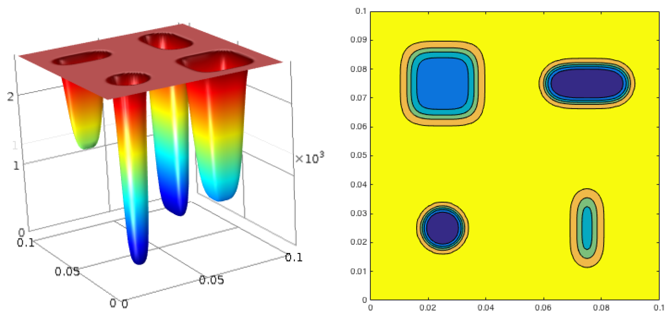
The upper surface is uniformly illuminated with a source with a power density W m, constant in time. The contact resistance between the slabs is due to a variable thickness . Given the thermal conductivity of the material between the two sheets (air: ), the unknown heat exchange coefficient is given by . Figure 1 shows the unknown heat exchange coefficient.

Figure 1.
Unknown heat exchange coefficient at the interface: graph and contour plot.
A gaussian noise with has been added to the simulated temperature map.
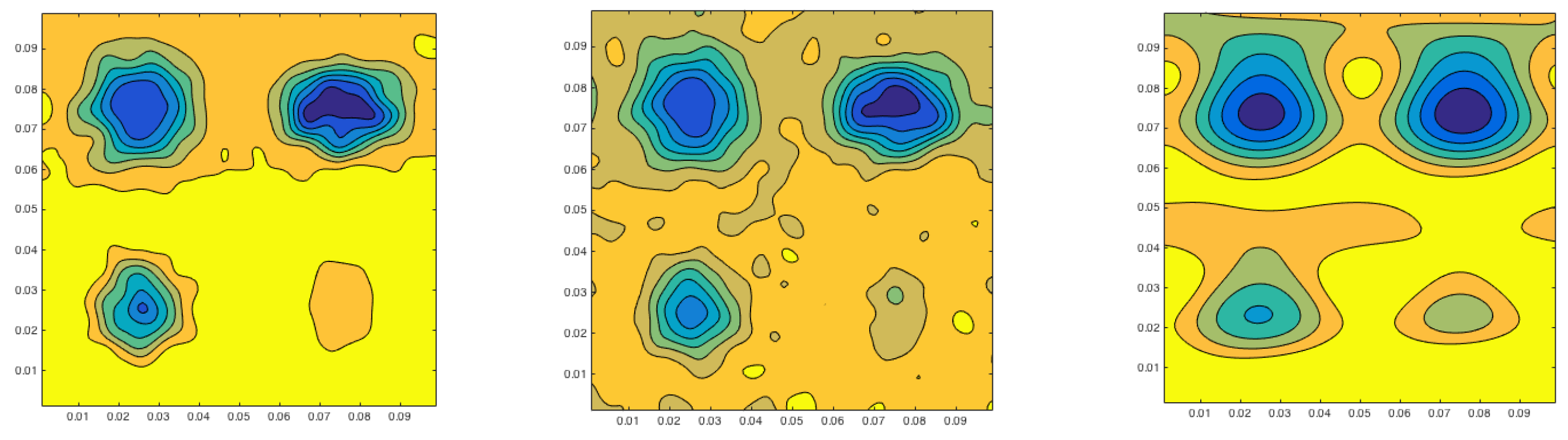
Figure 2 shows the reconstructed effective heat transfer coefficient without and with noise. In order to compute the spatial derivatives in the procedure, a cubic smoothing spline is applied to data when computing the first-order derivatives. Moreover, the same kind of smoothing is applied to temperature maps when noise is present. An alternative to data smoothing is FFT filtering the noisy data.
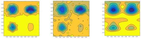
Figure 2.
Reconstructed without noise; with noise; with noise and a Fourier-filtered map. To be compared with the contour plot in Figure 1.
6. Discussion
In this paper we describe a method of active thermography for the numerical evaluation of defects of an inaccessible interface that divides two slabs in a composite. The method is based on the expansion of temperature (of the specimen) and thermal conductance (of the interface) in power of the thickness of one of the slabs. A perturbative technique (Thin Plate Approximation), already used in different contexts, is adapted to this problem. We deal with an ill-posed Inverse Problem for heat equation. Moreover, the computation of derivatives of discrete functions is required. In simulations, functions and derivatives are smoothed by means of FFT Filtering. Further developments: testing with experimental data (in progress, collaboration with Civil Engineering Dept. University of Parma), better mathematical modeling of the limit from interphase to interface (in progress, collaboration with Mathematical Department of the University of Firenze).
Funding
This research received no external funding.
Conflicts of Interest
The authors declare no conflict of interest.
References
- Javili, A.; Kaessmair, S.; Steinmann, P. General Imperfect Interfaces. Comput. Methods Appl. Mech. Eng. 2014, 275, 76–97. [Google Scholar] [CrossRef]
- Maldague, X.P.V. Theory and Practice of Infrared Technology for Nondestructive Testing; John Wiley and Sons: New York, NY, USA, 2001. [Google Scholar]
- Hashin, Z. Thin interphase/imperfect interface in conduction. J. Appl. Phys. 2001, 89, 2261. [Google Scholar] [CrossRef]
- Colaco, M.J.; Alves, C.J.S. A Backward Reciprocity Function Approach to the Estimation of Spatial and Transient Thermal Contact Conductance in Double-Layered Materials Using Non-Intrusive Measurements. Numer. Heat Transf. Part A Appl. 2015, 68, 117–132. [Google Scholar] [CrossRef]
- Inglese, G.; Olmi, R. Nondestructive evaluation of spatially varying internal heat transfer coefficients in a tube. Int. J. Heat Mass Transf. 2017, 108, 90–96. [Google Scholar] [CrossRef]
- Incropera, F.P.; Dewitt, D.P.; Bergman, T.L.; Lavine, A.S. Principles of Heat and Mass Transfer, 7th ed.; Wiley: Singapore, 2003. [Google Scholar]
- Inglese, G.; Olmi, R.; Scalbi, A. Characterization of a vertical crack using Laser Spot Thermography. Inverse Probl. Sci. Eng. 2020, 28, 1191–1208. [Google Scholar] [CrossRef]
Publisher’s Note: MDPI stays neutral with regard to jurisdictional claims in published maps and institutional affiliations. |
© 2021 by the authors. Licensee MDPI, Basel, Switzerland. This article is an open access article distributed under the terms and conditions of the Creative Commons Attribution (CC BY) license (https://creativecommons.org/licenses/by/4.0/).