Performance Analysis of Position Estimation and Correction Methods ^†

Abstract

There are several global and local position estimation and refinement techniques based on the GNSS (Global Navigation Satellite System) and environmental monitoring (e.g., LIDAR, Light Detection and Ranging). These are usually based on a combination of multiple sensors using some form of sensor fusion, together with a filtering or observation technique. The behavior of these algorithms may vary depending on the applied sensor signals and on their accuracy under different environmental conditions and for different vehicle types. In the case of systems that also use GNSS signals, different procedures must also be prepared for signal dropouts and, in the worst case, drastic fluctuations in accuracy. The aim of this research is to present and compare the performance of different estimation procedures for different vehicles and environmental conditions.

1. Introduction

The position estimation is one of the most important parts of autonomous and semi- autonomous vehicle research. The crucial part of research is the development of more accurate localization algorithms and the best possible refinement of position data. Several methods have been developed to improve the accuracy of Global Navigation Satellite System (GNSS) position data. The drawback of commercially available universal systems (which are based on the GNSS and Inertial Measurement Units (IMUs)) is always that they have limited ability to consider vehicle dynamics and are generally not able to use the vehicle’s internal sensors in the estimation and refinement process.

GNSS-based positioning systems, such as GPS, Galileo, Glonass and BeiDou, use satellites and ground receivers to achieve position data. The pure satellite-based positioning can be accurate to within tens of meters, depending on environmental disturbances (e.g., buildings, clouds, smog) and satellite visibility [1]. In order to increase the accuracy of purely satellite-based positioning, various techniques are used, for example, using ground-based transmission towers placed in known positions.

These methods, such as SBASs (Satellite-Based Augmentation Systems), DGNSS (Differential GNSS), PPP (Precise Point Positioning) and RTK (Real-Time Kinematic) can significantly increase the accuracy of “traditional” purely satellite-based positioning [1].

However, the disadvantage of these methods is that they require intermittent or continuous communication and connectivity between the vehicle and the system of base stations. The advantage is that they are universal, i.e., they can be used on any vehicle, but they cannot take advantage of the “limitations” of the vehicle’s design and cannot use sensor data from the vehicle.

To overcome these problems, algorithms have been developed that consider data from several different sensor systems and provide more accurate results than methods that work solely with GNSS and IMU data [2,3,4,5]. The earliest and most widely used localization techniques are based on GNSS, IMU and odometry data. Some sensors were originally designed for environmental monitoring, but they can be used for localization. LIDAR (Light Detection and Ranging), radar, ultrasound and vision systems such as mono and stereo cameras are excellent examples. Sensor fusion can be implemented in several ways, including using a Kalman filter or a particle filter, which can be used to achieve high accuracy with relatively low computational complexity [6,7,8,9].

The accuracy of the algorithms depends largely on the applied sensors, the models and the procedures used for sensor fusion. The aim of this research is to investigate how the less and more complex estimation procedures perform under real measurement conditions and whether they are suitable for use in embedded environments.

2. Estimation Algorithms

Different standalone estimation algorithms were developed based on sensor fusion techniques. These estimators can be used in different driving and environmental circumstances. Our goal was to test and integrate these procedures into a unified estimator algorithm capable of automatically switching between different them. The sensor fusion between GNSS and vehicle sensors is implemented by algorithms using an extended Kalman filter (EKF) based on a kinematic or dynamic model, which can be used to improve the accuracy of positioning and to replace satellite positioning for a shorter period.

System integration involved the synchronization of several algorithms and automatic switching between them [10,11]: kinematic model-based estimation without GNSS, kinematic model-based estimation with GNSS, dynamic model-based estimation without GNSS and dynamic model-based estimation with GNSS (

Table 1. The available sensor signals.

Signal	Symbol	Comment
Vehicle velocity [m/s]	v
Steering angle [rad]	δ
Longitudinal acceleration [m/s2]	ax
Lateral acceleration [m/s2]	ay
Yaw rate [rad/s]	$\dot{\psi }$
Longitudinal position [m]	x	Needed only for GNSS-based algorithms.
Lateral position [m]	y	Needed only for GNSS-based algorithms.

and

Table 2. The available vehicle parameters.

Parameter	Symbol	Comment
Front axle distance from center of gravity [m]	l1
Rear axle distance from center of gravity [m]	l2
Wheelbase [m]	l	l = l1+ l2
Vehicle mass [kg]	m
Steering ratio [-]	iS	Can be non-constant.
Front cornering stiffness [N/°]	c1
Front cornering stiffness [N/°]	c2
Yaw inertia [kg m2]	Jzz

).

2.1. Kinematic Model-Based Estimation

The basis of the kinematic model was introduced in [10,11]. The main equations of the kinematic model are

$$\beta =\mathrm{atan}\left({\displaystyle \frac{l_2}{l}}\tan \delta \right),$$

(1)

$$a_x=\mathrm{d}{v}_x/\mathrm{d}t \mathrm{and} a_y=\mathrm{d}{v}_y/\mathrm{d}t,$$

(2)

$$v_y=v_x\tan \beta ,$$

(3)

$$\dot{\psi }={\displaystyle \frac{v_x}{l_2}}\tan \beta ,$$

(4)

where β is the side-slip angle, v_x is the longitudinal velocity and v_y is the lateral vehicle velocity. During the modeling, it can be assumed that

$$\mathrm{d}x/\mathrm{d}t=v_x\cos \psi -v_y\sin \psi \mathrm{and} \mathrm{d}y/\mathrm{d}t=v_y\cos \psi +v_x\sin \psi ,$$

(5)

$$\mathrm{d}\psi /\mathrm{d}t=\dot{\psi },$$

(6)

where ψ is the yaw angle.

The extended Kalman filter can be created using the model equations as a basis and state, input and output vectors are the following:

$$\overline{x}=\left[\begin{array}{c}{v}_x\\ v_y\\ \psi \\ x\\ y\end{array}\right], \overline{u}=\left[\begin{array}{c}{a}_x\\ a_y\\ \delta \\ x\\ \dot{\psi }\end{array}\right], \overline{y}=\left[\begin{array}{c}\dot{\psi }\\ v_x\\ v_y\\ x\\ y\end{array}\right] , \mathrm{if} \mathrm{GNSS} \mathrm{available}, \overline{y}=\left[\begin{array}{c}\psi \\ v_x\\ v_y\end{array}\right] \mathrm{if} \mathrm{GNSS} \mathrm{unavailable}.$$

(7)

2.2. Dynamic Model-Based Estimation

The basis of the dynamic model was introduced in [10,11]. The main equations of dynamic model are based on the single-track model [2]:

$$\left[\dot{\begin{array}{c}\beta \\ \ddot{\psi }\end{array}}\right]=\left[\begin{array}{cc}-{\displaystyle \frac{c_1+c_2}{m v_x}}& {\displaystyle \frac{c_2{l}_2-c_1{l}_1}{m {\left(v_x\right)}^2}}-1\\ {\displaystyle \frac{c_2{l}_2-c_1{l}_1}{J_{zz}}}& -{\displaystyle \frac{c_1{l}_1^2+c_2{l}_2^2}{v_x{J}_{zz}}}\end{array}\right]\left[\begin{array}{c}\beta \\ \dot{\psi }\end{array}\right]+\left[\begin{array}{c}{\displaystyle \frac{c_1}{m v_x}}\\ {\displaystyle \frac{c_1{l}_1}{J_{zz}}}\end{array}\right]\delta ,$$

(8)

The extended Kalman filter can be created using the model equations as a basis and state, input and output vectors are the following:

$$\overline{x}=\left[\begin{array}{c}\beta \\ \dot{\psi }\\ \psi \\ x\\ y\end{array}\right], \overline{u}=\left[\begin{array}{c} v_x\\ \delta \end{array}\right], \overline{y}=\left[\begin{array}{c}\dot{\begin{array}{c}\psi \\ \psi \end{array}}\\ a_y\\ x\\ y\end{array}\right] \mathrm{if} \mathrm{GNSS} \mathrm{available}, \overline{y}=\left[\begin{array}{c}\dot{\begin{array}{c}\psi \\ \psi \end{array}}\\ a_y\end{array}\right] \mathrm{if} \mathrm{GNSS} \mathrm{unavailable}.$$

(9)

2.3. Integrated Algorithm

The difficulty of the switch is that the transition between algorithms must be made without a major position jump. Basically, the switching depends on the speed of the vehicle from the odometry and the accuracy of the GNSS. The switch between kinematic or dynamic model-based procedures occurs when the vehicle speed exceeds or falls below 2 m/s. The maximum recommended speed for the kinematic model-based methods can be determined by calculations, but experience shows that a value between 2 and 3 m/s is still appropriate for most vehicles [1]. The applicability of the GNSS is determined by whether an SBAS or a better correction method is available at that moment (

Table 3. Algorithm selection in the integrated method.

	Kinematic Model-Based Algorithm	Dynamic Model-Based Algorithm
GNSS signal enabled	The vehicle speed is less than 2 m/s and a minimum SBAS correction is available	Vehicle speed greater than or equal to 2 m/s and a minimum SBAS correction is available
GNSS signal disabled	The vehicle speed is less than 2 m/s and a minimum SBAS correction is unavailable	Vehicle speed greater than or equal to 2 m/s and a minimum SBAS correction is unavailable

).

The integrated method was implemented as an ROS (Robot Operating System) node in C++ programming language, intended to be easily adaptable to existing environments supporting the development of autonomous systems [12,13]. To decrease the hardware requirements for running the algorithms, optimized vector and matrix operations were used in the implementation. The maximum memory footprint of the integrated algorithm was below 8 MB, with a maximum CPU usage of 5% on NVIDIA Jetson Xavier hardware with an Ubuntu Linux operating system.

3. Measurement Results

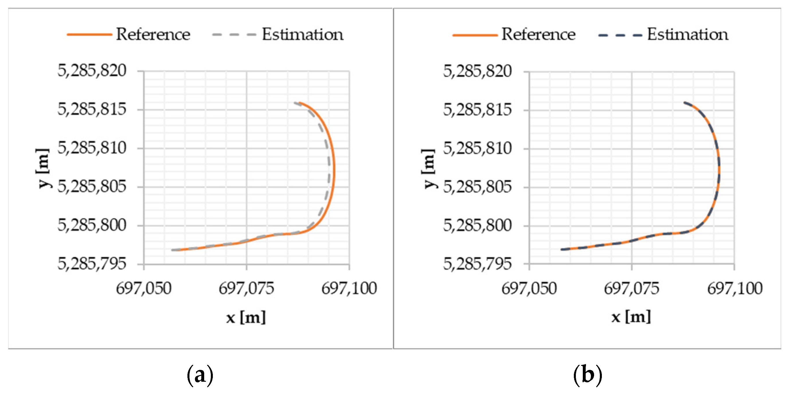
The first measurements were carried out on a Lexus SUV (

Table 4. The parameters of Lexus SUV.

Parameter	Value
Front axle distance from center of gravity	1.236 m
Rear axle distance from center of gravity	1.553 m
Wheelbase	2.789 m
Vehicle mass	2300 kg
Yaw inertial	4500 kg m2

) during a simple maneuver, and the results are shown in the Figure 1, with the GNSS signals switched on and off. All sensor signals shown in Table 1 were available during the measurements.

The algorithm produced good results with the GNSS signal on and off (the maximum of absolute position error was 0.7 m). As expected, with a sufficiently accurate GNSS signal, the estimation became more accurate (the maximum of absolute position error was 0.1 m).

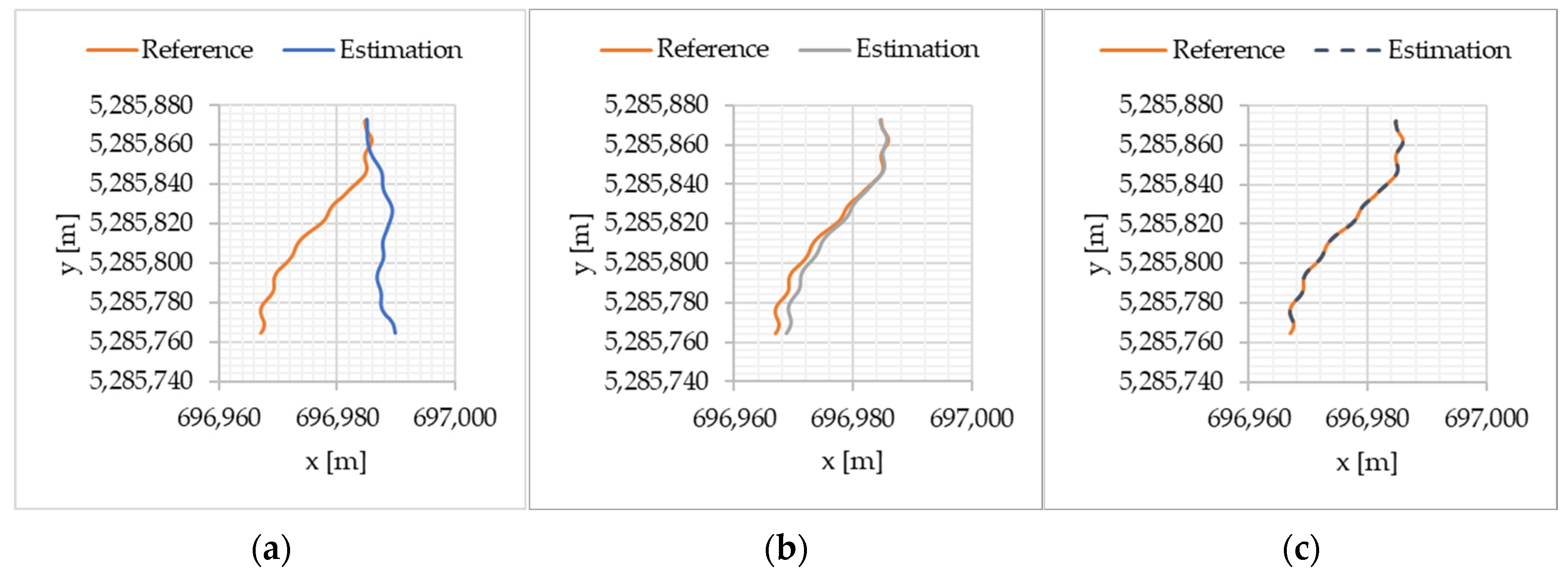
The fault tolerance of the algorithm was tested using a misplaced IMU. The IMU was rotated 15–20° around the y axis, which resulted in an offset in the acceleration signals. All built-in filtering and correction procedures were disabled in the sensors to ensure that, in addition to the offset values, they were also highly noisy. The sensor signals for these measurements are shown in the figures below (Figure 2).

Longitudinal acceleration shows a clear shift in value, and high noise can be observed in all acceleration values.

To illustrate fault tolerance, the results of a purely model-based procedure without an EKF are shown. The pure model-based method accumulated serious errors (the maximum of absolute position error was 23.6 m), while the EKF-based versions gave good results (the maximum of absolute position error was 3.4 m) (Figure 3).

4. Summary

During this research, the performance of position estimation procedures based on extended Kalman filters was successfully investigated. It was demonstrated that by integrating the different algorithms, an efficient estimation method can be created. The developed method is able to automatically switch between different algorithms without a major position jump in the filtered or estimated position data. Furthermore, to prove its efficiency, the runnability of the algorithms is tested on an embedded system.

References

- Tang, X.; Li, B.; Du, H. A study on dynamic motionplanning for autonomous vehicles based on nonlinear vehicle model. Sensors 2023, 23, 443. [Google Scholar] [CrossRef] [PubMed]
- Al Malki, H.H.; Moustafa, A.I.; Sinky, M.H. An improving position method using extended Kalman filter. Procedia Comput. Sci. 2021, 182, 28–37. [Google Scholar] [CrossRef]
- Cramariuc, A.; Bernreiter, L.; Tschopp, F.; Fehr, M.; Reijgwart, V.; Nieto, J.; Cadena, C. maplab 2.0—A modular and multi-modal mapping framework. IEEE Robot. Autom. Lett. 2023, 8, 520–527. [Google Scholar] [CrossRef]
- Kim, T.; Park, T.H. Extended Kalman filter (EKF) design for vehicle position tracking using reliability function of radar and lidar. Sensors 2020, 20, 4126. [Google Scholar] [CrossRef] [PubMed]
- Culley, J.; Garlick, S.; Esteller, E.G.; Georgiev, P.; Fursa, I.; Vander Sluis, I.; Bradley, A. System design for a driverless autonomous racing vehicle. In Proceedings of the 2020 12th International Symposium on Communication Systems, Networks and Digital Signal Processing (CSNDSP), Porto, Portugal, 20–22 July 2020. [Google Scholar]
- Montani, M.; Ronchi, L.; Capitani, R.; Annicchiarico, C. A hierarchical autonomous driver for a racing car: Real-time planning and tracking of the trajectory. Energies 2021, 14, 6008. [Google Scholar] [CrossRef]
- Schratter, M.; Zubaca, J.; Mautner-Lassnig, K.; Renzler, T.; Kirchengast, M.; Loigge, S.; Watzenig, D. Lidar-based mapping and localization for autonomous racing. In Proceedings of the 2021 International Conference on Robotics and Automation (ICRA 2021)–Workshop Opportunities and Challenges with Autonomous Racing, Xi’an, China, 30 May–5 June 2021. [Google Scholar]
- Xiao, X.; Biswas, J.; Stone, P. Learning inverse kinodynamics for accurate high-speed off-road navigation on unstructured terrain. In Proceedings of the 2021 International Conference on Robotics and Automation (ICRA 2021)—Workshop Opportunities and Challenges with Autonomous Racing, Xi’an, China, 30 May–5 June 2021. [Google Scholar]
- Montenbruck, O.; Steigenberger, P.; Hauschild, A. Comparing the ‘Big 4’–A User’s View on GNSS Performance. In Proceedings of the 2020 IEEE/ION Position, Location and Navigation Symposium (PLANS), Portland, OR, USA, 20–23 April 2020. [Google Scholar]
- Markó, N.; Horváth, E.; Szalay, I.; Enisz, K. Deep Learning-Based Approach for Autonomous Vehicle Localization: Application and Experimental Analysis. Machines 2023, 11, 1079. [Google Scholar] [CrossRef]
- Enisz, K.; Szalay, I.; Horváth, E. Localization robustness improvement for an autonomous race car using multiple extended Kalman filters. Proc. Inst. Mech. Eng. Part D J. Automob. Eng. 2024; accepted. [Google Scholar] [CrossRef]
- Detta, G. Integration of Matlab-based controllers with ROS for autonomous agricultural vehicles. Ph.D. Thesis, Politecnico di Torino, Turin, Italy, 2022. [Google Scholar]
- Macenski, S.; Foote, T.; Gerkey, B.; Lalancette, C.; Woodall, W. Robot operating system 2: Design, architecture, and uses in the wild. Sci. Robot. 2022, 7, eabm6074. [Google Scholar] [CrossRef] [PubMed]