Abstract
The oil and gas industries are facing several industry-specific barriers which include process improvements, ignorance of complex operations, equipment management, logistics operations, etc. However, the enormous amount of data that are being produced by this industry, and the implementation of analytics, can overcome these challenges. This project aims to put forth a step-by-step procedure to preprocess data and utilize data analytics tools to provide meaningful insights to make business intelligent decisions for companies. The results from this research will be presented in data preprocessing procedures, the use of analytics, and machine learning applications in the O&G industry.
1. Introduction
The natural gas consumption rate on a global scale is rising significantly. According to statistics, around 39% of the USA’s electric power supply came from natural gas in 2023, and this is expected to fall to 37% in 2024. Due to the nature of its lower production of greenhouse gases, its utilization rate has been rising. The cheapest way to transfer natural gas is through pipelines. However, this is sometimes more prone to cause accidents. There could be several causes that can damage the pipelines like the substance of the pipelines, age of the pipelines, and operating circumstances, to name a few [1]. Damage in the pipes can lead to leakages of the oil, which could potentially cause human loss, impacting companies’ finances, or could be dangerous to the environment [2]. In 2019 alone, there were 11 fatalities in addition to USD 333 million in damages caused by pipeline accidents. For the past 30 years, the US has faced nearly USD 7 billion in property damage because of the leakage issues of pipelines. These industries are in deserted areas with extreme weather conditions. Hence, it is difficult for humans to keep an eye on any leakages. So, several studies have been conducted to tackle and detect gas leakages to prevent disasters.
The very first leak detection approach based on pressure and flow measurements was created by Billmann et al. [3]. Another popular technique is the concept of the negative pressure wave (NPW) utilized by Reinaldo et al. [4]. Other than these, the accelerometer [5], the distributed temperature system (DTS) [6], time–domain reflectometry [7], the passive acoustic-based system [8], and computational fluid dynamics (CFD) [9] have been proposed by various authors. However, the uses of AI [10] and machine learning [11] are growing in popularity in this era. Several machine learning models have been implemented to detect leakages in pipelines, controlling the effect of pollution from leakages.
For example, Laurentys et al. [12] used genetic algorithms, fuzzy logic, neural networks, and statistical analysis for dependable leakage detection in a Brazilian petroleum installation. Qu et al. [13] provided a prior warning system in terms of pipe leaks with machine learning. They used a support vector machine model which provided good accuracy. Carvalho et al. [14] utilized artificial neural networks (ANNs) and magnetic flux leakage (MFL) signals for leak detection and achieved a success rate of 71.7%. Ibitoye et al. [15] employed a convolutional neural network model for leak detection on video images captured using IoT cameras. Liu et al. [16] utilized a gaussian extreme learning machine (GELM), a well-known ML algorithm, to detect water distribution network (WDN) leakage recognition. Kanoun et al. [17] used SVM, DT, RF, GBDT, AdB, and XGB models to anticipate the failure in a refinery pipeline based on nine predictor variables. Their XGB model achieved an accuracy of 99.7%. Zhao et al. [18] proposed a multi-scale residual networks (MSRNs) model to detect leaks in a liquid-filled pipeline. Harati et al. [19] applied five ML models, SVR, KNNR, DTR, RFR, and ANN, to predict the location and size of probable leaks. Though corrosion defect is one of the key driving factors that create leakages in pipelines, very little work has been conducted on predicting the corrosion level based on several predictors. The objectives of this assessment are given as follows:
- Briefly discuss and justify the use of the three different ML models, namely, decision tree, k-nearest neighbors (KNN), and random forest.
- Briefly discuss data preprocessing steps and their importance in machine learning.
- Apply those machine learning models to predict the pipeline corrosion level for pipeline leakages.
- Make a comparison based on several parameters like accuracy, sensitivity, and precision.
The rest of this paper progresses as follows: Section 2 consists of a data description, followed by data preprocessing steps in the Section 3. Section 4 elaborates on the machine learning models, and the result analysis section is discussed in the Section 5. Finally, this paper ends with a conclusion and a discussion of implications in the Section 6.
2. Methodology
The methodology here includes the steps in building a machine learning algorithm. The very first step is data collection and preprocessing. The next step is training with the clean data by using the desired algorithms and finally assessing the model performance by using the model parameters. Here, the study discusses various methods to clean or preprocess the data and also three different types of machine learning algorithms. The k-nearest neighbors (KNN), decision tree, and random forest algorithms are discussed. This research aims to study the purposes of and differences between these algorithms and how they are used to detect leakages in pipelines.
Data Collection
An open source dataset was used for this research. The dataset for data analytics and ML purposes was collected from a single source or location for this study. The dataset chosen for this research has 8000 rows with 4 columns (pressure, rate of flow, temperature, corrosion defect). Here, the input variables are the rate of flow, temperature, and pressure, whereas the output variable is the corrosion level. The corrosion defect variable is given as high vs. low. Using the input variables, this study discusses how to predict the output variable and, based on that, how to detect the leakages in pipelines.
3. Data Preprocessing
The data generated in the real world are incomplete, with missing values, errors, or outliers, and are not clean and consistent. When the analysis is performed on such data, the results obtained can be incorrect, biased, and misleading. Hence, cleaning the data before running analytics or predictive modeling is necessary. This section provides a detailed overview of the data collection, cleaning, preprocessing, and removal, and a few more methods that make it more usable and efficient for our models.
3.1. Data Cleaning
Data cleaning is the essential first step in the machine learning modeling process. This approach guarantees more accurate and significant results by converting unrefined, inconsistent, or insufficient information into a polished, useable state. This phase goes beyond just “cleaning” the data; it also ensures that the data more closely reflects real-world trends and reduces noise, which in turn produces better, more trustworthy insights and predictions.
3.2. Missing Values
Missing or null values in the dataset cannot be ignored as a lot of analysis or machine learning models do not accept or handle missing fields. There are several ways to handle missing entries. The missing values can be excluded from the dataset. This method is generally followed when the dataset has very few missing values or blanks. The missing values can also be filled manually by using several statistical methods such as mean imputation or median imputation. Manually filling in the missing values is generally time-consuming and sometimes also prone to several errors. Mean imputation can be a preferred method over median imputation. Another simple method to fill in the missing values is replacing the blanks with a zero. The missing values can also be imputed by using the backward or forward filling process where the very next number or value or the previous value is used to fill the missing values. One of the most generally used methods, using a simple algorithm to predict the actual values, can also be used.
3.3. Outlier or Noisy Data Detection
Outliers are the observations in the dataset that vary strongly from other data points. There can be various reasons why the data can have outliers, due to faults while collecting the data, errors while manually entering the data, sometimes system or tools errors, errors due to data sampling, etc. The outliers must be identified to build a robust machine learning algorithm. For example, in the oil and gas summary production sample dataset, there are several outliers or faulty data due to the above-termed errors. For example, one data point in the year column is 202, the active oil wells column, which should have either Y/N, has a Z in one of the fields, and the corrosion level for one data point is 100 where all the others are between 0 and 1. These examples are outliers which are identified during the data preprocessing step. Outliers can be detected by using box plots, Z-scores, etc.
3.4. Data Transformation
Normalization is a technique to scale the features in the range between 0 and 1. This helps in improving the performance of the model and provides accurate and unbiased results from analysis and model building. Data transformation from an old data point to a new data point is shown in Equation (1) below.
Here, Y′ indicates the new value of Y. The above equation normalizes the data and converts them into a range [0, 1].
4. Machine Learning Models
Once the data are cleaned using the above steps, machine learning models are built. To start building the models, the clean dataset is divided into train and test data. The data are generally divided using ratios (8:2) or percentages (70%:30%). Generally, the training sample is allotted more of the dataset than the test. The train data are used to train the model, help it learn the features of the dataset, and improve the model, while the test data are used to test the model performance using various model parameters.
4.1. Decision Tree Classifier
The data used for this study’s purpose have various attributes including the rate of flow, temperature, and pressure of flow, as well as the corrosion level (high/low). High corrosion leads to gas leakages whereas low corrosion does not. Here, to detect the leakages, a decision tree classifier is used to predict the leakages. A decision tree is a hierarchical data structure that represents data through a divide-and-conquer strategy [20].
The decision tree algorithm uses features to output high corrosion level/low corrosion level to determine gas leakages and continuously splits the data until it isolates all the points to a particular class. This entire process organizes the data in the form of a tree and hence it is called the decision tree classifier. The tree starts with a root node and splits further into child nodes every time the tree answers a question. In using decision trees as a classifier, the goal is to construct the tree that represents the data to determine the labels for the new data.
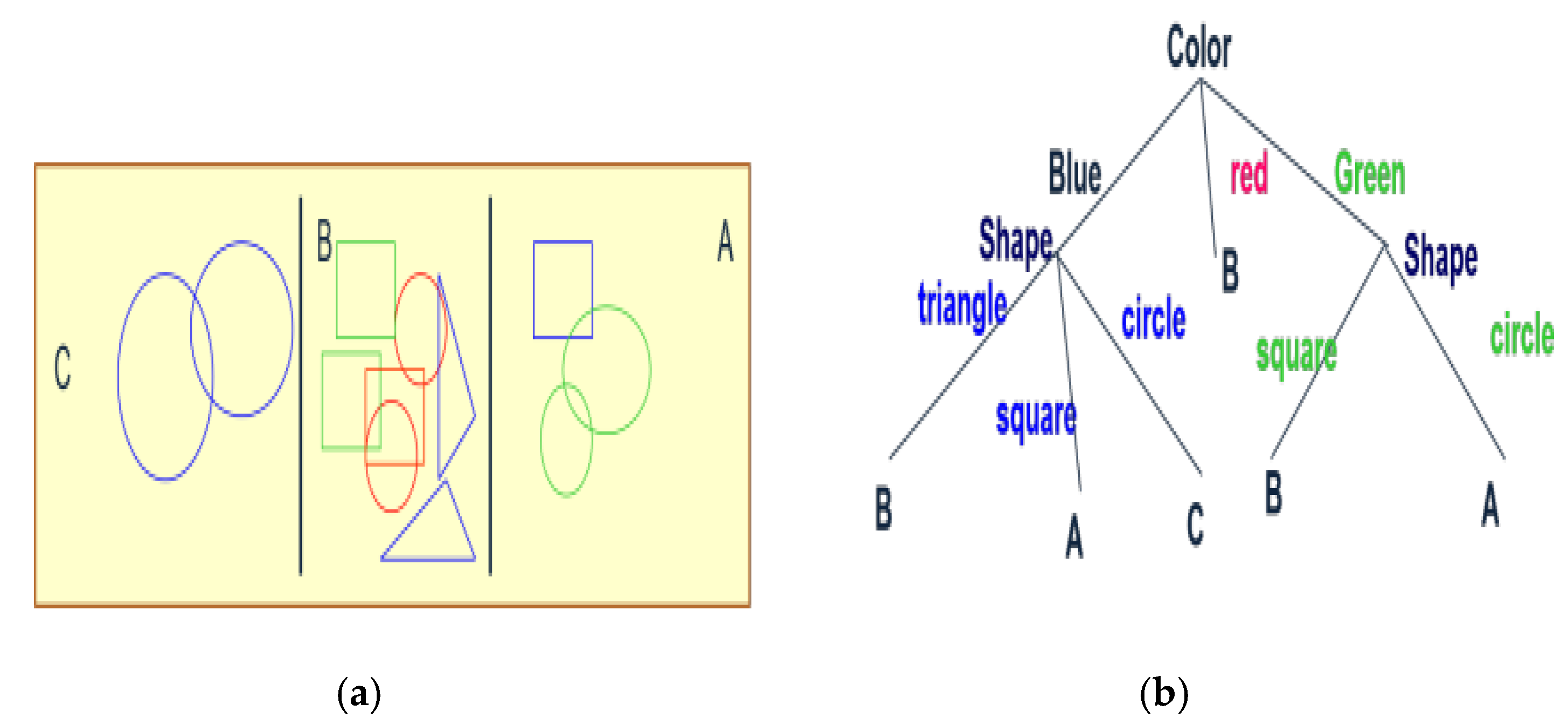
In a machine learning model, features are the characteristics of the data. It can be a feature vector like the above Figure 1a (e.g. color, shape, label). Every internal node denotes a choice in Figure 1b (such as “Is the color blue?”), and branches result in various conclusions like reaching labels A, B, or C, depending on the responses. The main reason behind the use of the decision tree model is it can capture the nonlinear relationships among the predictors (temperature, flow rate, pressure) which is not possible for linear models. Also, this model is capable of dealing with relationships between the predictors and understanding the intricate dynamics of corrosion in pipelines.
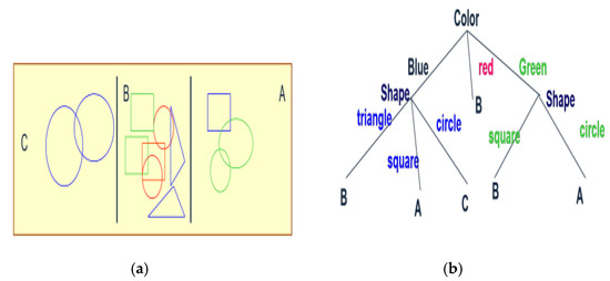
Figure 1.
Example of a decision tree [20].
4.2. K Nearest Neighbor
The k-nearest neighbor (KNN) is a type of machine learning algorithm that can be used for both regression as well as classification types of predictions. In the classification technique, the output is classified into a specific class, determined by the values of its neighbors [21]. The output class is determined by the class that is most common among the neighbors closest to the output. The KNN algorithm is a simple yet powerful algorithm to classify the output variables. The best way to describe this algorithm is whenever there are new data, it classifies the output based on its k-nearest neighbors.
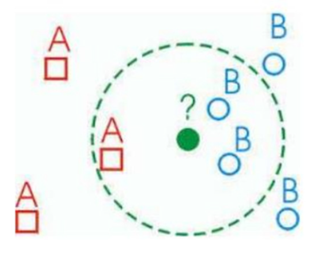
From Figure 2, A represented by red squares and B represented by blue circle are two different classes or categories of data points in a classification model. While the green dot is the unknown data point that we want to classify based on its neighbors either A or B. The KNN algorithm has been utilized because it is proficient in utilizing the local structure of the data which enables it to effectively identify close features of the pipelines. It also provides the flexibility to determine the size (K) of the neighborhood to cope with diverse density and variability levels, which helps to increase the sensitivity of our model. It also has various advantages with missing values and noisy data.
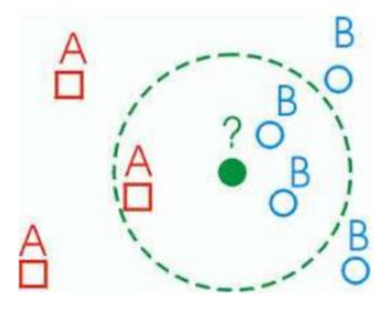
Figure 2.
Classifying a new data point based on the neighbors [21].
4.3. Random Forest
The random forest algorithm is one of the most popular and most powerful machine learning algorithms [22]. The random forest method is a simple extension of the decision tree algorithm. The algorithm fixes the issue that the decision tree classifier has and, hence, it is one of the most powerful classification techniques. When new data need to be classified, the random forest method plugs in the data to all the decision trees. Each tree classifies the new data to either high corrosion level/low corrosion level. The random forest method takes the majority from all the decision trees and classifies the output.
The reason behind using this powerful model is that the model can prevent overfitting, along with increasing generalizability. This model is also effective on high-dimensional datasets with lots of predictive features. As it is a combination of multiple decision trees, it is more resistant to noise and outliers in detecting corrosion levels than an individual decision tree.
4.4. Model Performance Metrics
Three performance metrics, accuracy, sensitivity, and precision, have been considered for the models. The details are given as follows:
The accuracy of a model is defined as how many samples are truly predicted out of all the samples.
where TP = true positives, TN = true negatives, FP = false positives, and FN = false negatives.
Precision is defined as what percentage of all positive predictions are truly predicted.
where TP = true positives, TN = true negatives, FP = false positives, and FN = false negatives.
Sensitivity is defined as what percentage of positive predictions among all the positive samples.
where TP = true positives, TN = true negatives, FP = false positives, and FN = false negatives.
5. Result Analysis
The decision tree (DT), random forest (RF), and K nearest neighbor (KNN) models are discussed in this study to detect the leakages of oil/gas from pipelines. After all the discussed models are run on the data, Table 1 below draws a comparison between each of the models based on all the different model parameters; finally, the best model is chosen based on the model performance metrics.

Table 1.
Performance metrics.
The above table shows the comparison of model parameters such as the accuracy, sensitivity, precision, and F-score of the model. Amongst the three discussed machine learning models, the random forest model outperformed the other models in determining the corrosion level in the data, whereas the KNN model underperformed in terms of all cases. The RF model detected the corrosion level with a 91.55% accuracy, which indicates the model was able to predict approximately 91.55% of corrosion levels perfectly. The DT model had an 87.13% accuracy, which was somewhat higher than the KNN model, which had only an 84% accuracy. The RF model again achieved a sensitivity score of 92% which means that, among all the positive corrosion level cases, our model was able to predict 92% of them correctly. The DT and KNN models had 5% and 8% lower scores, respectively, than the RF model. Lastly, for the precision score, the RF model accurately predicted 92%. This implies that, out of all the positive cases it predicted, 92% of the cases were truly positive. Meanwhile, the DT and KNN models had the same scores as before, 87% and 84%, respectively. Hence, whenever we use those models with unseen data with the same predictor variable and run the model, it will predict the low corrosion (no leakage) or high corrosion (detecting leakage) perfectly.
6. Conclusions
Overall, the DT and RF models had higher performance scores than the KNN model. This reveals they are adept at capturing complicated non-linear correlations among the predictor and target variables. On the other hand, the KNN model depends solely on the distance across the data points, so it might be difficult for it to handle complex correlations. The RF and DT models also perform well in high-dimensional areas with lots of predictor variables. However, the KNN model is prone to being affected by high dimensionality which means, as the number of features rises, the distance between the nearest neighbors diminishes. Also, while the RF and DT methods withstand anomalies and noisy data, the KNN model cannot, as it depends on distance.
In this research, one of the issues faced by the oil and gas industry is discussed. Oil and gas companies face the issue of leakages of oil or gas in their pipelines. To tackle this issue, a step-by-step approach is demonstrated to build machine learning algorithms that can detect these leakages. A general dataset with few features is taken into account and the model is built on that dataset. Three types of machine learning algorithms are discussed, and the best algorithm is picked based on comparing the different model evaluation parameters. Using these models, a system can be developed to identify and detect such leakages based on real-time data. Whenever the data are input into the system, the model will be able to detect unusual activity. The main outcome of this is our model can suggest which pipelines need a preventive maintenance approach by detecting the corrosion level. Additionally, it can locate vulnerable pipelines so that authorities give more priority to that zone and minimize the use of resources and time. Finally, necessary precautions can be taken and potential harm to the environment or human life can be avoided.
The current limitation of this research is that the data are limited to only metal pipelines, as corrosion generally occurs due to the chemical reactions between metal and the environment. Plastic or other materials are corrosion-proof, so it will be possible for those models to work with data where the pipeline is made of plastics if the predictor variables and target variables are assigned accordingly, such as to ultraviolet (UV) radiation, high temperature, or mechanical stress, to name a few. For future work, the authors would like to work on the plastic pipeline degradation prediction model and make a comparison between the two pipeline materials.
Author Contributions
Conceptualization, A.M. and F.R.; methodology, A.M. and F.R.; software, A.M.; validation, A.M., F.R., A.M.S. and N.U.I.H.; formal analysis, A.M.; investigation, A.M.S.; resources, A.M.; data curation, A.M. and A.M.S.; writing—original draft preparation, A.M. and F.R.; writing—review and editing, A.M.S. and N.U.I.H.; visualization, A.M. and F.R.; supervision, A.M.S. and N.U.I.H.; project administration, A.M.S. and N.U.I.H. All authors have read and agreed to the published version of the manuscript.
Funding
This research received no external funding.
Institutional Review Board Statement
Not applicable.
Informed Consent Statement
Not applicable.
Data Availability Statement
Data sharing is not applicable due to privacy.
Conflicts of Interest
The authors declare no conflict of interest.
References
- Mamlook, R.; Al-Jayyousi, O. Fuzzy sets analysis for leak detection in infrastructure systems: A proposed methodology. Clean Technol. Environ. Policy 2003, 6, 26–31. [Google Scholar] [CrossRef]
- Cruz, R.P.D.; Silva, F.V.D.; Fileti, A.M.F. Machine learning and acoustic method applied to leak detection. Clean Technol. Environ. Policy 2020, 22, 627–638. [Google Scholar] [CrossRef]
- Billmann, L.; Isermann, R. Leak Detection Methods for Pipelines. Automatica 1987, 23, 381–385. [Google Scholar] [CrossRef]
- Silva, R.A.; Buiatti, C.M.; Cruz, S.L.; Pereira, J.A. Pressure wave behaviour and leak detection in pipelines. Comput. Chem. Eng. 1996, 20, S491–S496. [Google Scholar] [CrossRef]
- Jin, H.; Zhang, L.; Liang, W.; Ding, Q. Integrated leakage detection and localization model for gas pipelines based on the acoustic wave method. J. Loss Prev. Process Ind. 2014, 27, 74–88. [Google Scholar] [CrossRef]
- Wang, L.; Narasimman, S.C.; Ravula, S.R. Water Ingress Detectionin Low-Pressure Gas Pipelines Using Distributed Temperature. Sensing System. IEEE Sens. J. 2024, 17, 3165–3173. [Google Scholar] [CrossRef]
- Cataldo, A.; Cannazza, G.; Benedetto, E.D.; Giaquinto, N. A New Method for Detecting Leaks in Underground Water Pipelines. IEEE Sens. J. 2012, 12, 1660–1667. [Google Scholar] [CrossRef]
- Mahmutoglua, K.T.Y. A passive acoustic based system to locate leak hole in underwater natural gas pipelines. Digit. Signal Process. 2018, 76, 59–65. [Google Scholar] [CrossRef]
- Li, X.; Chen, G.; Zhang, R.; Zhu, H.; Fu, J. Simulation and assessment of underwater gas release and dispersion from subsea gas pipelines leak. Process Saf. Environ. Prot. 2018, 119, 46–57. [Google Scholar]
- Ali, S.M.; Rahman, A.U.; Kabir, G.; Paul, S.K. Artificial Intelligence Approach to Predict Supply Chain Performance: Implications for Sustainability. Sustainability 2024, 16, 2373. [Google Scholar] [CrossRef]
- Khan, M.M.; Bashar, I.; Minhaj, G.M.; Wasi, A.I.; Hossain, N.U.I. Resilient and sustainable supplier selection: An integration of SCOR 4.0 and machine learning approach. Sustain. Resilient Infrastruct. 2023, 8, 453–469. [Google Scholar] [CrossRef]
- Laurentys, C.; Bomfimb, C.; Menezes, B.; Caminhas, W. Design of a pipeline leakage detection using expert system: A novel approach. Appl. Soft Comput. 2011, 11, 1057–1066. [Google Scholar] [CrossRef]
- Qu, Z.; Feng, H.; Zeng, Z.; Zhuge, J.; Jin, S. A SVM-based pipeline leakage detection and pre-warning system. Measurement 2010, 2010, 513–519. [Google Scholar] [CrossRef]
- Carvalho, A.; Rebello, J.; Sagrilo, L.; Camerini, C.; Miranda, I. MFL signals and artificial neural networks applied to detection and classification of pipe weld defects. NDT E Int. 2006, 39, 661–667. [Google Scholar] [CrossRef]
- Ibitoye, O.; Shafiq, M.O.; Matrawy, A. A Convolutional Neural Network Based Solution for Pipeline Leak Detection. In Proceedings of the 2019 IEEE International Conference on Wireless for Space and Extreme Environments, Ottawa, ON, Canada, 16–18 October 2019. [Google Scholar]
- Liu, M.; Guo, G.; Xu, Y.; Yang, Y.; Liu, N. Performance of Improved Gaussian Extreme Learning Machine for Water Pipeline Leak Recognition. IEEE Sens. J. 2024, 24, 8474–8483. [Google Scholar] [CrossRef]
- Kanoun, Y.; Aghbash, A.M.; Belem, T.; Zouari, B.; Mrad, H. Failure prediction in the refinery piping system using machine learning algorithms: Classification and comparison. Procedia Comput. Sci. 2024, 232, 1663–1672. [Google Scholar] [CrossRef]
- Zhao, S.-L.; Zhou, L.-H.; Liu, S.-G.; Dong, L.-Q.; Hong, Z.; Zhao, D.; Guo, C. Liquid-filled pipeline leak detection and localization based on multi-scale residual networks. Meas. Sci. Technol. 2024, 35, 055012. [Google Scholar] [CrossRef]
- Harati, S.; Gomari, S.R.; Rahman, M.A.; Hassan, R.; Hassan, I.; Sleiti, A.K.; Hamilton, M. Enhancing Safety in Geological Carbon Sequestration: Supervised Machine Learning for Early Detection and Mitigation of CO2 Leakage in Injection Wells. In Proceedings of the International Petroleum Technology Conference, Dhahran, Saudi Arabia, 12–14 February 2024. [Google Scholar]
- Roth, D. Decision Trees. CS 446 Machine Learning Fall 2016. cis.upenn.edu. 2016. Available online: https://www.cis.upenn.edu/~danroth/Teaching/CS446-17/LectureNotesNew/dtree/main.pdf (accessed on 10 October 2024).
- Bennett, M.; Casey, H.; Atsu, K. A Binary Classification of Beatles Song Authorship. cs229.stanford.edu. 2014. Available online: https://cs229.stanford.edu/proj2014/Miles%20Bennett,%20Casey%20Haaland,%20Atsu%20Kobashi,Classification%20Of%20Beatles%20Authorship.pdf (accessed on 10 October 2024).
- Brownlee, J. Bagging and Random Forest Ensemble Algorithms for Machine Learning. Machine Learning Algorithms. Machine Learning Mastery. 2020. Available online: https://machinelearningmastery.com/bagging-and-random-forest-ensemble-algorithms-for-machine-learning/ (accessed on 10 October 2024).
Disclaimer/Publisher’s Note: The statements, opinions and data contained in all publications are solely those of the individual author(s) and contributor(s) and not of MDPI and/or the editor(s). MDPI and/or the editor(s) disclaim responsibility for any injury to people or property resulting from any ideas, methods, instructions or products referred to in the content. |
© 2024 by the authors. Licensee MDPI, Basel, Switzerland. This article is an open access article distributed under the terms and conditions of the Creative Commons Attribution (CC BY) license (https://creativecommons.org/licenses/by/4.0/).