Abstract
In the transition from non-renewable to renewable energy sources, wind and solar power plants have emerged as primary sources for reducing atmospheric emissions. However, ensuring grid stability remains a challenge in the absence of traditional power plants. Renewable energy sources are often referred to as “inertia-less,” highlighting their vulnerability in transient stability scenarios in which system inertia is crucial. This paper introduces the concept of “synthetic inertia estimation” using an Extended Kalman Filter as a novel solution. Using the synthetic inertia estimation from a wind power plant, one can use the residual kinetic energy, and through the DC/AC converter, inject it into the system during times of stability disturbances. This paper offers practical insights into synthetic inertia estimation and its implementation for enhancing grid stability in a sustainable energy landscape.
1. Introduction
Nowadays, when talking about the transition from non-renewable to green, renewable energy, it is usually referred to the transition to wind and solar power plants as the main sources of electrical energy, which would reduce the emission of harmful substances into the atmosphere. Looking at the specific power available, wind power plants are particularly attractive, as today’s generators exceed 10 MW of power per installed unit [1,2]. In addition, the goal of the International Commission on Climate Change is that, by 2050, 30% of electricity production will come from wind farms, which further supports efforts to build as many wind farms as possible [3].
In such circumstances, there is often a recognized requirement for a more robust base power plant that plays a crucial role in upholding power system stability. This is achieved through the swift response of power unit controllers when standard operational conditions are disrupted. It should be noted that renewable energy power plants lack this capability, which becomes particularly evident in transient stability problems, during which the inherent inertia of the power system’s generators is of utmost importance [4]. Therefore, many authors often refer to renewable sources that are connected to the grid via power electronic devices as inertia-less sources [5]. This also includes the wind power plants, although they have rotating generators. It should be noted that, the most common and efficient wind power generators are connected to the power system through a full-scale converter, which separates them from the grid with a DC link.
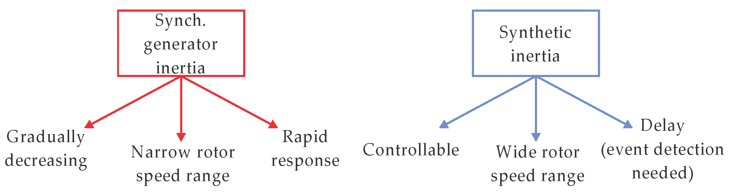
However, if one abandons the classical thinking that the moment of inertia is the product of the mass and the square of the equivalent diameter of the rotating body, and thinks only about its effect and importance in transient situations, one can arrive at a new concept, which is called synthetic inertia. This term can be considered as a virtual moment of inertia and should not be confused with the term virtual power plants. If a power park mimics the moment of inertia from another rotating generator power source, through its power electronic components, then it can be said that that power park uses the synthetic inertia [6].
In order to introduce the term synthetic inertia and to analyze its benefits, it is best to identify it through residual kinetic energy that cannot disappear in moments when the production unit is not used, such as in cases of transient and fault phenomena, which usually disrupt the power system’s stability.
However, the distinction between synthetic inertia and a traditional single generator’s moment of inertia can be observed in Figure 1.
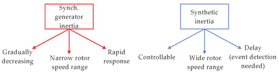
Figure 1.
Comparison of synchronous generator inertia and synthetic inertia.
To date, most authors have presented possible solutions to the potential exploitation of synthetic inertia through block diagrams in the management structure of wind power plants, where works such as [7,8,9,10,11] stand out. It should be noted that, in order to utilize the potential of synthetic inertia, fast measurements from PMU (Phase Measurement Unit) devices are required [12]. This is combined with dynamic state estimation algorithms which are used for nonlinear estimation problems that cannot be approximated.
In the following sections of this paper, an expression for the calculation of synthetic inertia will be derived, based on the generator’s swing equation. Then, using the Extended Kalman Filter, the estimation of the synthetic inertia in different operating conditions of the system is attempted, and all of this is performed using real measurements with PMU devices installed in the Austrian power grid. In addition, at the end, a proposal to use the calculated moment of inertia for stability problem analysis is offered, which will be included in future work.
2. Synthetic Inertia Calculation and Estimation
2.1. Synthetic Inertia Constant
In order to calculate the required synthetic inertia constant, which will be used in the stability analysis, one must start with the swing equation for a classic synchronous generator.
In this context, J stands for the cumulative moment of inertia for all rotating masses, αm denotes the acceleration of the rotor’s angular velocity, while Tm, Te, Ta represent the mechanical torque produced by the prime mover, electrical torque corresponding to the generator’s three-phase power output, and the net accelerating torque, respectively [13].
Since J can have many values, stability analysis often employs a new constant known as the normalized inertia constant, denoted as H. This approach helps constrain the values to a narrower range, typically between 1 and 10 (p.u.). It is defined as:
where Srated represents the rated apparent power of the unit and ωmsync is the mechanical synchronous rotating speed.
Considering that the power system consists of many generators, it is essential to establish shared dynamic performance metrics. Once the individual generators have reached a stable state, their frequencies blend and converge to create the system’s frequency. To capture the collective dynamic behaviour of the entire system, the system’s inertial constant, denoted as Hsys is used. This parameter represents the cumulative inertial contributions as the weighted sum of all individual generator inertial constants, denoted as Hi [14].
The system’s reaction to disturbances and frequency deviations is linked to its total inertia. Consequently, the Rate of Change of Frequency (RoCoF) is a derivative of the frequency signal and is closely related to the system’s inertial response. The calculation of RoCoF can be expressed as:
where f is the frequency of the system (Hz), fs is the nominal frequency (Hz), and the ΔP is the power imbalance in the system [14].
Synthetic inertia can be associated with the deliberate provision of electrical torque from a unit, which is proportionate to the Rate of Change of Frequency (RoCoF) at the unit’s terminals [14]. With the combination of the previous equations, one can derive the equation for the calculation of the synthetic inertia constant for some arbitrary generator i.
The derived equation can be used to calculate the power from the inertia-less-source-like wind power plant in order to support the system in cases of stability crisis. The Hsynth,i is the required synthetic inertia constant, which will be estimated in this paper and can be used to provide frequency and rotor-angle stability support to the power system.
The authors of [15] concluded that the maximum synthetic inertia of a wind power generator cannot exceed 10% of the pre-event energy equivalent.
2.2. Extended Kalman Filter Algorithm
The power system is inherently nonlinear, making the application of a conventional Kalman filter estimation inappropriate. To address this issue, specialized Nonlinear Kalman Filters have been designed specifically for nonlinear problems, such as power system estimation. One notable example of these nonlinear estimation algorithms is the Extended Kalman Filter, often referred to as a dynamic state estimation algorithm.
If a nonlinear system is described by the difference equation and the observation model with added noise, it can be written as:
where xk is the state of interest, yk is an observation vector, f(∙) is the process’ nonlinear vector function, h(∙) is the observation nonlinear vector function.
The initial state x0 can be a random vector with a known mean value µ0 = E[x0] and covariance P0 = E[(x0 − µ0)(x0 − µ0)T], both calculated as expected values. Random vector wk captures uncertainties in the model and vk denotes the measurement noise, and they are uncorrelated [16].
The main steps of Extended Kalman Filter for the nonlinear system can be summarized as:
- Initialization step to calculate the state variable and state covariance matrix P0 as expected values.
- 2.
- Prediction step conducted for each time step.
This step consists of the following sub steps:
- Calculation of partial derivative matrices for the current state estimate:
- b.
- Propagation of the estate estimate and the covariance estimate
- 3.
- Update/correction step.
This step consists of the following sub steps:
- a.
- Calculation of partial derivative matrices for correction with linearization
- b.
- Updated measurement of the state estimate and estimation error covariance using Kalman gain
- c.
- Updated measurement of the state estimate and estimation error covariance using Kalman gain
2.3. Proposed Estimation Procedure
With the aforementioned information, one can deduce a procedure for the synthetic inertia estimation using the Extended Kalman Filter. As expected, knowledge about the power system at the start of estimation is needed, together with information about the wind power plant and the rated parameters.
The main parts are the PMU measurements, primarily because of their rapid data acquisition and the extensive data required for transient scenarios and event timing. These measurements are transmitted to the Dynamic State Estimator, which uses the Extended Kalman Filter to estimate synthetic inertia for wind power plants. Subsequently, the estimated data serve as the target function for the wind power plant’s output power control unit. This approach enables the wind power plant, equipped with a full-scale converter and separated from the grid via the DC link, to inject the necessary power into the system, thereby aiding during transient or rotor angle-stability issues when they occur.
3. Measurements and Estimation Results
In order to demonstrate the procedure of the proposed algorithm for wind power plants’ synthetic inertia estimation, a wind power plant with a single turbine is taken into account. Some data about the wind power plant turbine are provided in Table 1.

Table 1.
Wind power plant turbine data.
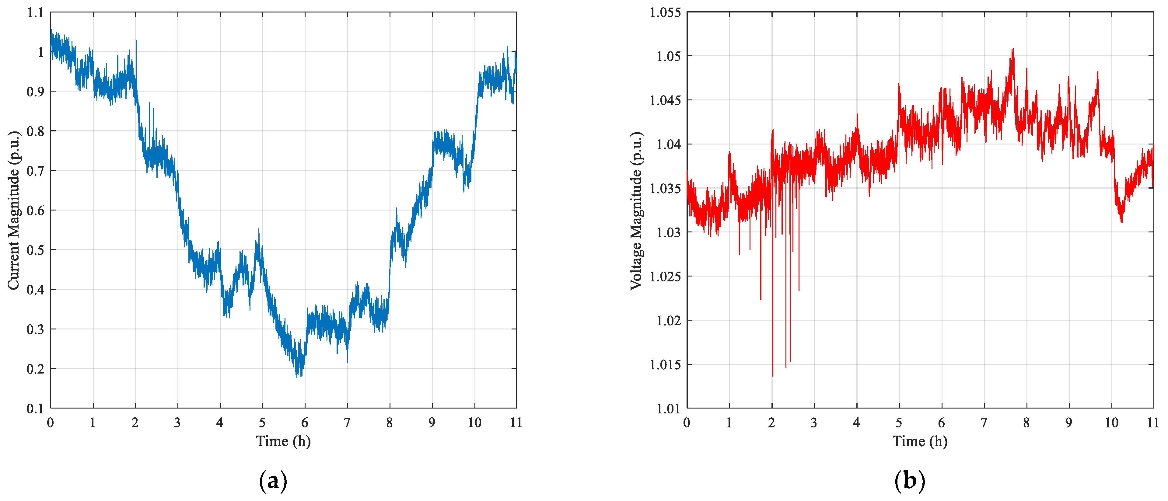
The measurements with the PMU device were conducted for 11 (h) and the data were prepared for the Extended Kalman Filter estimation of the synthetic inertia. The magnitudes of voltage and current, measured with the PMU device, are shown in Figure 2.

Figure 2.
Current magnitudes measured with the PMU device (a); voltage magnitude measured with the PMU device (b).
During the measurement day, in the period between 1 p.m. and 3 p.m., there was a storm near the measuring point. This can particularly be seen in the voltage measurements shown. It is these transients that are needed to show the changes in synthetic inertia that occur according to the dependence on the change in frequency presented. For this reason, the following analysis will focus on the period from 1 p.m. to 3 p.m., during which 36,000 PMU measurement samples have been acquired.
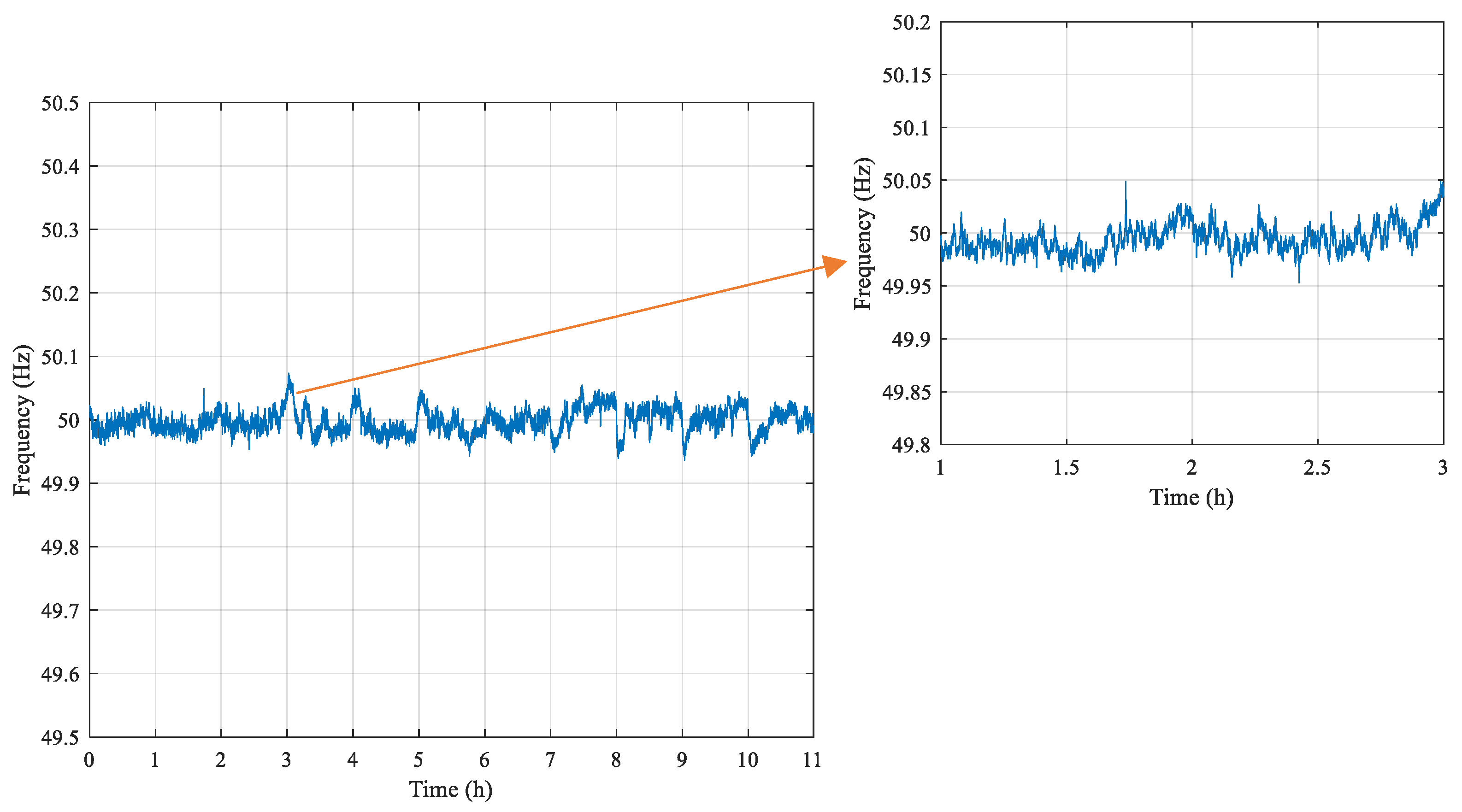
In the stability analysis, the most important variable is the system’s frequency. The PMU device measured the frequency at the measurement site, and its change can be seen in Figure 3.
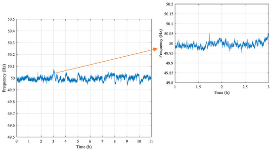
Figure 3.
Frequency measured with the PMU device.
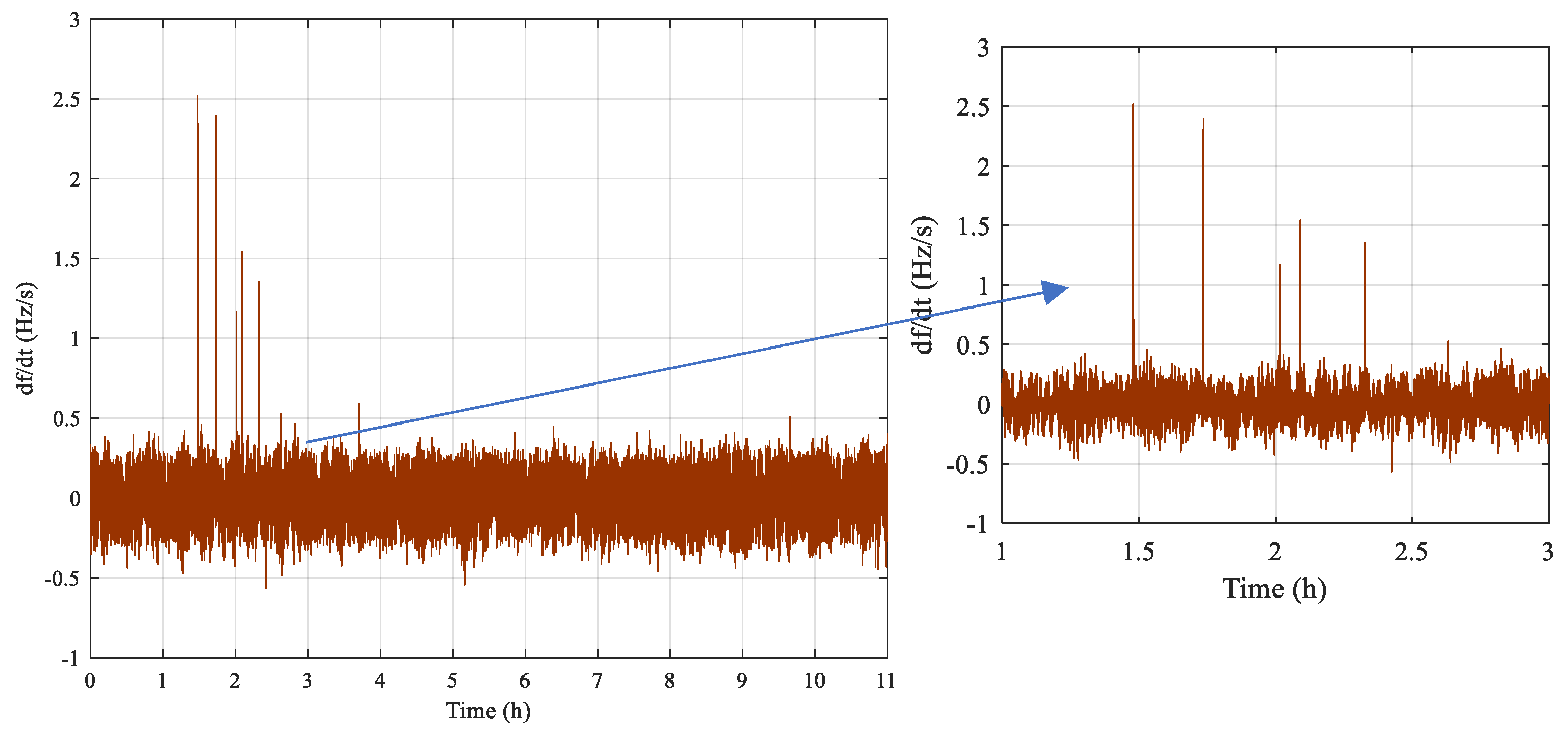
The frequency change plays a crucial role in the synthetic inertia estimation; therefore, a measurement for that variable is needed. The frequency change data measured with the PMU device is presented in Figure 4.

Figure 4.
Frequency change measured with the PMU device.
Figure 4 shows a heavy rate of frequency changes during the storm period from 1 p.m. to 3 p.m. with highest rate of change in frequency reaching 2.51 (Hz/s).
For a set of 36,000 samples of PMU measurements, in a period from 1 p.m. to 3 p.m., and by using the Extended Kalman Filter algorithm, the synthetic inertia of the used wind power plant was estimated using the previously mentioned relations. The diagonal elements of the process’ noise covariance matrix Q and measurement noise covariance matrix R are set to value 0.001 for the sake of estimation.
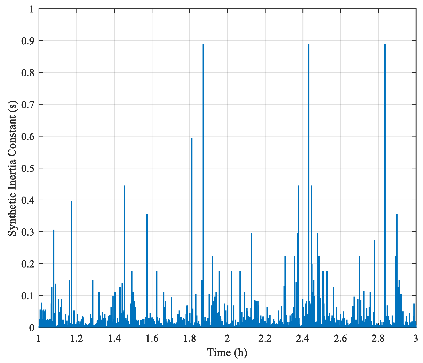
The estimated synthetic inertia constant change can be seen from the Figure 5.
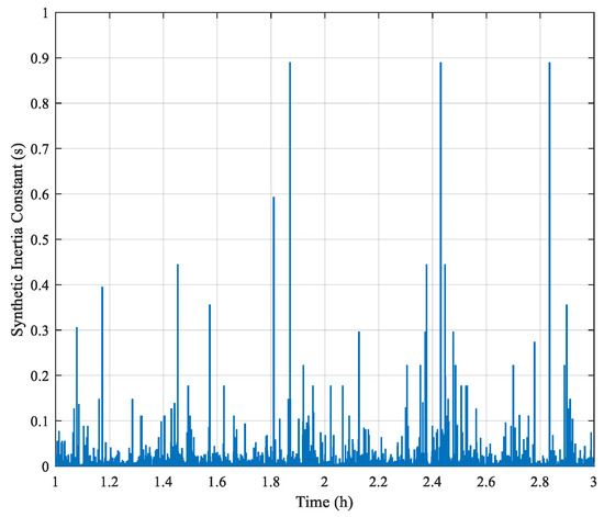
Figure 5.
Estimated synthetic inertia constant for the wind power plant turbine between 1 p.m. and 3 p.m. on the day of measurement.
It should be noted that, the Extended Kalman Filter algorithm effectively tracked voltage magnitudes and phase angles in comparison to the measured ones, even during transient conditions. Accuracy assessments showed that the estimated states closely matched high-precision synchrophasor measurements, with an average root mean square error of less than 0.1 degrees and 0.01 per unit for voltage magnitude. Uncertainty analysis indicated that state estimates were highly reliable, with 95% confidence intervals within tight bounds. Sensitivity analysis demonstrated that the algorithm maintained its performance even when subjected to variations in measurement noise levels, confirming its robustness for real-time grid monitoring and control.
It is necessary to pay attention to the fact that the constant of the synthetic inertia obtained has a high rate of change due to the measurements being taken every 20 (ms). This can lead to a deterioration in the power quality, though the main goal of using this power injection is to maintain the stability of the system. This implies that these two problems (system stability and power quality) cannot be fully separated.
The previous diagram shows that the highest frequency drops, seen in Figure 3 and Figure 4, resulted in high synthetic inertia constants, especially the three peak values, almost reaching the 10% margin of the standard inertia constant.
Although it seems that such changes are impossible to produce in a real power plant, rapid changes in synthetic inertia are possible in wind power plants due to the full-scale converter which, due to their small time constants, has the possibility of rapid changes in output power. This allows matching the power output with the estimated synthetic inertia constant, thereby achieving the required power injection at a given time.
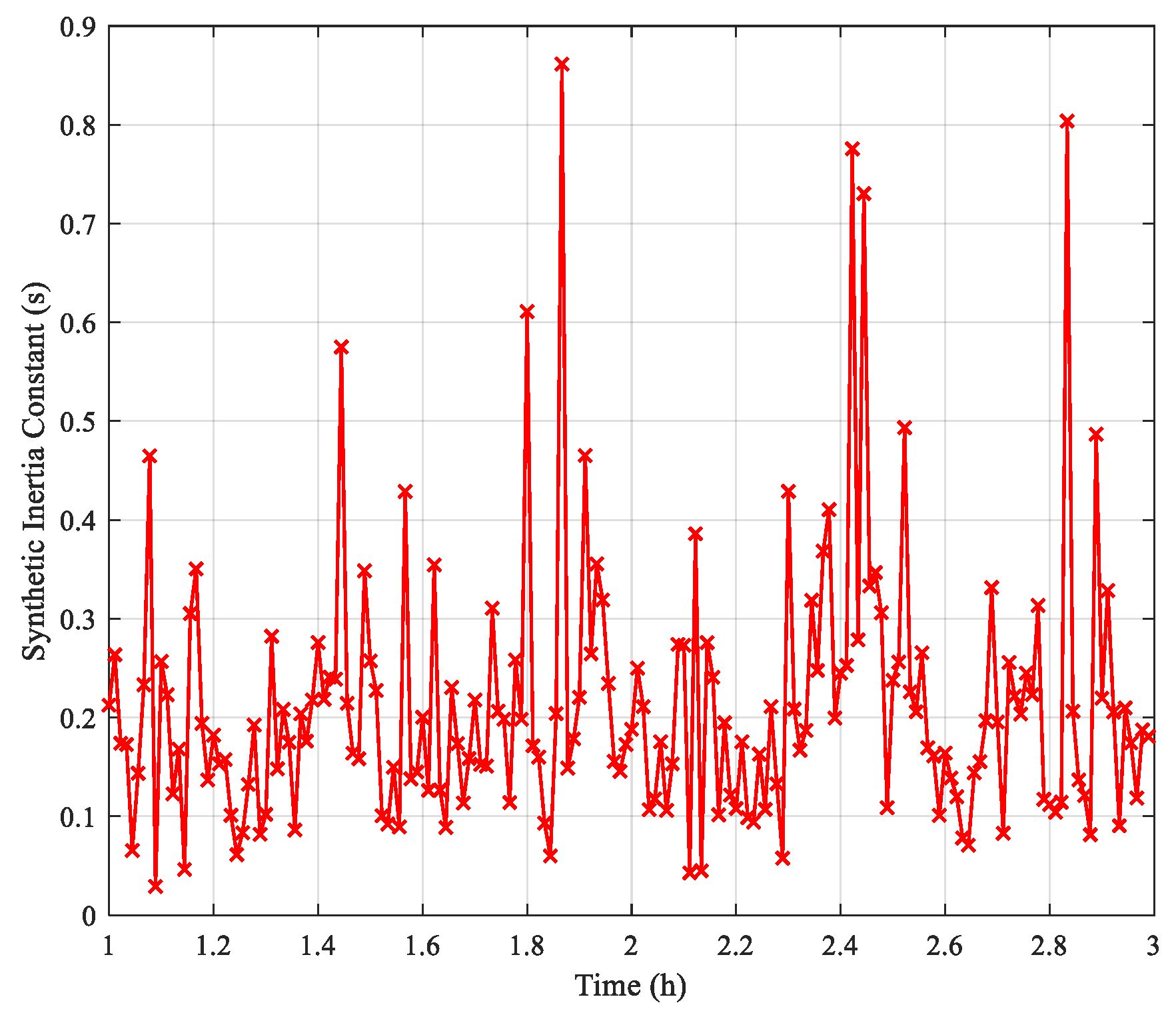
If needed, the rate of change in the estimated synthetic inertia can be filtered. In order to lower the rate change, a rate-limiting filter has been applied, and the results are shown on Figure 6.
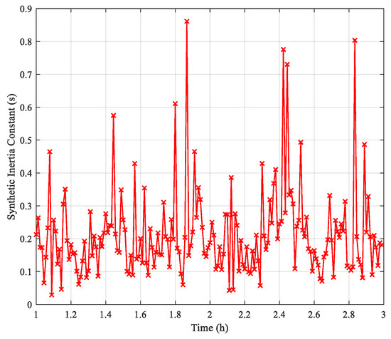
Figure 6.
Estimated synthetic inertia constant for the wind power plant turbine between 1 p.m. and 3 p.m. on the day of measurement, with the rate limit applied.
The mean value of the filtered synthetic inertia constant obtained from Figure 6 is 0.1845 (s). The highest value is 0.874 (s), while the lowest is 0.0365 (s). As expected, the peaks in the synthetic inertia constant during frequency dips are transmitted through the filter. This makes it possible for the power injection to have less-sudden changes. As said before, the synthetic inertia constant represents the stored kinetic energy which can be used to restore part of the power when the frequency starts to drop. Therefore, one can use the synthetic inertia as a pool of energy for critical situations.
4. Conclusions
Based on what has been presented, it can be concluded that, in the future, renewable sources will be able to be used to maintain the stability of the power system more than was originally thought. This further allows for an increase in the share of renewable energy sources in the overall production.
This paper shows that it is possible to estimate the synthetic inertia of a wind power plant based on fast measurements from a PMU device. In addition, one can conclude that it is also possible to emulate synthetic inertia for other renewable sources that have no moving parts. Of course, the availability of fast measurements, like those from the PMU, which SCADA systems cannot provide, is of crucial importance.
Synthetic inertia can be used as a measure of the available rotating power, which is usually not known by the system operator, and therefore not used to support the system when disturbances occur that disturb the stability of the system. Using synthetic inertia in this way can contribute to increasing the transient or rotor-angle stability of the system. Clearly, for this to work, it is necessary to have access to information about the synthetic inertia quickly when a disturbance occurs, which is provided by dynamic estimation of it with the help of PMU measurements. It should be noted that synthetic inertia depends mostly on the frequency change in the power system which makes it perfect for usage when huge stability disturbances occur.
Synthetic inertia acts as a crucial stabilizing force, preventing grid frequency deviations and voltage fluctuations. Essentially, it serves as a dynamic reservoir of energy, ready to respond within milliseconds.
Future work will include the use of other dynamic state estimation techniques such as the Unscented Kalman Filter with the aim of comparing it with the Extended Kalman Filter, improving efficiency and achieving better optimization. Additionally, an analysis of the application of synthetic inertia, estimated in the presented way, in real systems will be performed.
Author Contributions
Conceptualization, V.H. and H.R.; methodology, V.H.; software, V.H.; validation, V.H. and S.H.; formal analysis, V.H.; investigation, V.H.; resources, V.H. and H.R.; data curation, V.H. and H.R.; writing—original draft preparation, V.H.; writing—review and editing, V.H., H.R., and S.H.; visualization, V.H.; supervision, H.R.; project administration, H.R.; funding acquisition, V.H. All authors have read and agreed to the published version of the manuscript.
Funding
This research received no external funding.
Data Availability Statement
3rd Party Data Restrictions apply to the availability of these data. Data was obtained from Austrian Power Grid and are available [https://www.apg.at/] with the permission of Austrian Power Grid.
Conflicts of Interest
The authors declare no conflicts of interest.
References
- Bak, C.; Bitsche, R.; Yde, A.; Kim, T.; Hansen, M.H.; Zahle, F.; Gaunaa, M.; Blasques, J.P.A.A.; Døssing, M.; Wedel Heinen, J.-J.; et al. Light Rotor: The 10-MW reference wind turbine. In Proceedings of the EWEA, Copenhagen, Denmark, 16–19 April 2012. [Google Scholar]
- Gilbert, M.M. Renewable and Efficient Electric Power Systems; John Wiley & Sons: Hoboken, NJ, USA, 2013. [Google Scholar]
- Edenhofer, O.; Pichs-Madruga, R.; Sokona, Y.; Seyboth, K.; Arvizu, D.; Bruckner, T.; Christensen, J.; Chum, H.; Devernay, J.; Faaij, A.; et al. IPCC Special Report on Renewable Energy Sources and Climate Change Mitigation; Prepared by Working Group III of the Intergovernmental Panel on Climate Change; Cambridge University Press: Cambridge, UK, 2011. [Google Scholar]
- Kundur, P.; Balu, N.J. Power System Stability and Control, EPRI Power System Engineering Series; McGraw Hill: New York, NY, USA, 1994. [Google Scholar]
- Zhao, J.; Gómez-Expósito, A.; Netto, M.; Mili, L.; Abur, A.; Terzija, V.; Kamwa, I.; Pai, B.; Singh, A.K.; Qi, J.; et al. Power System Dynamic State Estimation: Motivations, Definitions, Methodologies, and Future Work. IEEE Trans. Power Syst. 2017, 34, 3188–3198. [Google Scholar] [CrossRef]
- ENTSO-E. Need for synthetic inertia (SI) for frequency regulation. In ENTSO-E Guidance Document for National Implementation for Network Codes on Grid Connection; ENTSO-E: Brussels, Belgium, 2017. [Google Scholar]
- Bo, W.; Chong, S.; Weicheng, S.; Guangru, Z.; Kaisong, D. Actual Measurement and Analysis of Wind Power Plant Participating in Power Grid Fast Frequency Modulation Base on Droop Characteristic. In Proceedings of the 2018 International Conference on Power System Technology (POWERCON), Guangzhou, China, 6–9 November 2018; pp. 1552–1557. [Google Scholar] [CrossRef]
- Shao, C.; Li, Z.; Hao, R.; Qie, Z.; Xu, G.; Hu, J. A Wind Farm Frequency Control Method Based on the Frequency Regulation Ability of Wind Turbine Generators. In Proceedings of the 2020 5th Asia Conference on Power and Electrical Engineering (ACPEE), Chengdu, China, 4–7 June 2020; pp. 592–596. [Google Scholar] [CrossRef]
- Jadeja, P.; Sood, V.K. Synthetic/virtual Inertia in Renewable Energy Sourced Grid: A Review. In Proceedings of the 2023 5th International Conference on Energy, Power and Environment: Towards Flexible Green Energy Technologies (ICEPE), Shillong, India, 8–9 March 2023; pp. 1–6. [Google Scholar] [CrossRef]
- Aragon, D.A.; Unamuno, E.; Muro, A.G.; Ceballos, S.; Barrena, J.A. Second-order Filter-based Inertia Emulation (SOFIE) for Low Inertia Power Systems. IEEE Trans. Power Deliv. 2023, 1–12. [Google Scholar] [CrossRef]
- Anusha, D.; De, D.; Tiwari, A.C.; Sahu, S. Modelling and Control of Synthetic Inertia Controller for Modular Multilevel Converter Fed HVDC Systems. In Proceedings of the 2023 5th International Conference on Energy, Power and Environment: Towards Flexible Green Energy Technologies (ICEPE), Shillong, India, 8–9 March 2023; pp. 1–6. [Google Scholar] [CrossRef]
- Helac, V.; Hanjalic, S.; Grebovic, S.; Becirovic, V. Synthetic Inertia in Wind Power Plants: An Overview. In Proceedings of the 2023 22nd International Symposium INFOTEH-JAHORINA (INFOTEH), East Sarajevo, Bosnia and Herzegovina, 15–17 March 2023; pp. 1–6. [Google Scholar] [CrossRef]
- Saccomanno, F. Electric Power Systems: Analysis and Control; IEEE Press: Piscataway, NJ, USA, 2003. [Google Scholar]
- Eriksson, R.; Modig, N.; Elkington, K. Synthetic inertia versus fast frequency response: A definition. IET Renew. Power Gener. 2018, 12, 507–514. [Google Scholar] [CrossRef]
- Knüppel, K.; Thuring, T.; Kumar, P.; Kragelund, S.; Nielsen, M.N.; André, R. Frequency Activated Fast Power Reserve for Wind Power Plant Delivered from Stored Kinetic Energy in the Wind Turbine Inertia. In Proceedings of the 10th International Workshop on Large-Scale Integration of Wind Power into Power Systems as well as on Transmission Networks for Offshore Wind Power Farms, Aarhus, Denmark, 25–26 October 2011. [Google Scholar]
- Dan, S. Optimal State Estimation: Kalman, H Infinity, and Nonlinear Approaches; John Wiley & Sons: Hoboken, NJ, USA, 2006. [Google Scholar]
- Terejanu, G.A. Extended Kalman Filter Tutorial. University at Buffalo: Buffalo, NY, USA, 2008. [Google Scholar]
Disclaimer/Publisher’s Note: The statements, opinions and data contained in all publications are solely those of the individual author(s) and contributor(s) and not of MDPI and/or the editor(s). MDPI and/or the editor(s) disclaim responsibility for any injury to people or property resulting from any ideas, methods, instructions or products referred to in the content. |
© 2024 by the authors. Licensee MDPI, Basel, Switzerland. This article is an open access article distributed under the terms and conditions of the Creative Commons Attribution (CC BY) license (https://creativecommons.org/licenses/by/4.0/).