Brain Signals to Actions Using Machine Learning ^†

Abstract

This research presents a machine learning model that predicts left, right, or no action using electroencephalography (EEG) signals extracted from two different wearable EEG headsets. The research aims to develop an accurate and efficient model by following a rigorous and effective process divided into two parts. In Part I, the constant features approach is employed, which involves data loading, feature extraction, preprocessing, model selection, and tuning the best model for optimal performance. The performance of classification algorithms (support vector machine (SVM), decision tree classifier, and random forest classifier) is evaluated using root-mean-squared error metrics. In Part II, the multivariate time series approach is utilized to improve the accuracy and robustness of the model. The approach involves data loading, preprocessing (such as normalizing the data), modeling, results analysis, and deployment preparation. A neural network architecture consisting of convolutional filters followed by a long short-term memory neural network (LSTM) is used in the proposed approach. The convolutional layer performs a convolution of an input series of feature maps with a filter matrix to extract high-level features. The LSTM network is specifically designed to capture long-term dependencies and overcome the issue of vanishing gradients. The proposed approach achieves an accuracy of 98% and can be used for real-time testing. The model can be utilized in various fields where accurate and real-time prediction of brain–computer interfaces (BCI) actions is crucial. Overall, the proposed approach provides a promising solution to the problem of action prediction using EEG signals, and further research can be conducted to explore its potential applications and optimize its performance.

1. Introduction

In recent years, there has been a growing interest in the development of machine learning (ML) algorithms for the control of robotic devices using electroencephalography (EEG) signals extracted from the brain [1,2]. For example, Schirrmeister et al. (2017) [3] conducted a study investigating the application of deep learning techniques, particularly convolutional neural networks (CNNs), for decoding EEG signals. The researchers utilized a large dataset of EEG recordings to train CNN models that could classify different mental states, such as motor imagery or attention levels. Their work showed that deep learning algorithms could effectively extract meaningful patterns from EEG data, improving the accuracy of decoding and enabling real-time BCI applications.

Isa et al. (2019) [4] conducted another study focusing on the classification of motor imagery in brain–computer interface (BCI) by using classifiers from machine learning techniques. The BCI system consists of two main steps, which are feature extraction and classification. The fast Fourier transform (FFT) features are extracted from the electroencephalography (EEG) signals to transform the signals into the frequency domain. Due to the high dimensionality of data resulting from the feature extraction stage, linear discriminant analysis (LDA) is used to minimize the number of dimensions by finding the feature subspace that optimizes class reparability. Five classifiers: support vector machine (SVM), K-nearest neighbors (KNN), Naïve Bayes, decision tree, and logistic regression are used in the study. The performance was tested by using Dataset 1 from BCI Competition IV, which consists of imaginary hand and foot movement EEG data. As a result, SVM, logistic regression, and Naïve Bayes classifier achieved the highest accuracy with 89.09% in AUC measurement.

The current approach has the potential to provide a more natural and intuitive way of controlling robotic devices, particularly for individuals with physical disabilities. In this paper, we present a step-by-step approach to develop an ML-based model for predicting a chosen action (right–none–left) using EEG signals extracted from the brain using the two different headsets for the potential control of robotic arms or other robotic devices. The approach involves collecting EEG data from participants, preprocessing the data, selecting an appropriate ML algorithm, training, and testing the model, and optimizing its performance if necessary. This paper aims to provide a comprehensive guide for researchers interested in developing ML-based models for the control of robotic devices using EEG signals.

2. Materials and Method

In this study, an ML-based model was developed to predict a chosen action (left, right, or none) using EEG signals extracted from the brain using two different headsets, the Emotiv EPOC(Manufacturer: Emotiv Inc., San Francisco, CA, USA) and OpenBCI(Manufacturer: OpenBCI Inc., New York, NY, USA).

The following steps were followed:

• Data Collection: EEG data were collected from participants while they performed a set of right, none, and left actions. The left action data were used to train and test the ML model.
• Data Preprocessing: The collected EEG data were preprocessed to remove any artifacts and noise, and to prepare it for further analysis.
• Model Selection: An appropriate ML algorithm was selected that could handle the complexity of the problem and the size of the dataset, such as support vector machines (SVM), decision trees, or artificial neural networks (ANN).
• Model Training: The selected ML algorithm was trained using the preprocessed EEG data and the engineered features. The performance of the trained model was evaluated using appropriate metrics, such as accuracy, precision, recall, and F1 score.
• Model Testing: The trained model was tested using a separate test dataset to evaluate its generalization performance and avoid overfitting.

Model Optimization: The parameters of the ML algorithm were optimized to improve its performance and generalization.

2.1. Data Collection

The specific brainwave patterns and signals were extracted from publicly available EEG data sources and were evaluated. These datasets contained a collection of EEG recordings capturing brain activity. The datasets were collected from publicly available EEG datasets in the OpenBCI and Emotiv EPOC. The datasets included motor imagery tasks involving the left hand, right hand, and no action. The datasets comprised different subsets as follows. The first source used was from the OpenBCI Community Dataset, obtaining data in February 2021 [5]. This subset involved 52 subjects, including 38 validated subjects with discriminative features. The second data source consisted of datasets extracted from the Emotiv EPOC headset used by the corresponding author in February 2021. The Emotiv EPOC is accompanied by a freely available software (Emotiv Control Panel) that provides the capability to analyze a subject’s brainwaves and develop a personalized cognitive signature which corresponds to each particular action, in this case left and right, as well as the background state (neutral state or no action). However, it is important to note that these particular datasets are no longer available to the public due to their temporary nature.

In this study, fast Fourier transform (FFT) analysis was employed to extract frequency-domain information from the EEG signals. The application of FFT facilitated the transformation of the EEG time-domain data into the frequency-domain representation, enabling the identification of distinctive spectral components. FFT (fast Fourier transform) is a mathematical technique used in this study to allow for the transformation of the time-domain signal into the frequency domain. That meant it would be able to provide a view of the number of signals enabled in each frequency. Then, the FFT algorithm would break down the time-domain signal into its component frequencies and show the amplitude (or power) of each frequency component. That would be helpful in identifying which frequencies were prominent in the signal and how they changed over time.

FFT is commonly used in brain wave signal processing because it allows for the analysis of the frequency content of a signal. Brain waves, which are electrical signals generated by the brain, can be quite complex and contain signals at different frequencies. By performing an FFT on the brain wave signal in this study, it was possible to break it down into its component frequencies and determine the power at each frequency. FFT can be used in BCIs to extract features from EEG signals that are related to specific mental states or actions, such as changes in the power of the alpha frequency range (8–12 Hz) that are associated with relaxation or attention.

To mitigate the influence of noise and artifacts present in the raw EEG signals, a preprocessing step was implemented. The fast Fourier transform (FFT) method was utilized to identify and isolate noise and artifact frequencies from the EEG data. By identifying abnormal frequency components that deviated from the typical neural oscillations, these unwanted signals were effectively attenuated. This process contributed to enhancing the signal quality and minimizing the potential interference caused by extraneous factors, ultimately improving the accuracy of subsequent analyses.

2.2. The Process

By adhering to the following process, the goal was to be attained in a scientifically rigorous and effective manner. The process was divided into two parts: in Part I, the constant features approach was utilized, while in Part II, the multivariate time series approach was used.

2.2.1. Part I: Constant Features Approach

In Part I, the constant features approach was used. The constant features approach was implemented through a series of steps. The process began by loading the data and then extracting the necessary features. Afterward, preprocessing techniques were applied, which included tasks like standardizing the data. Various models were experimented with to identify the most fitting one. Following this, the best model was fine-tuned, aiming to optimize its performance and achieve the best possible results.

The constant features technique was used to identify and remove features (or variables) that did not provide any information or predictive power to a model. The variance of each feature across the dataset was checked. If a feature had no variance, meaning that its value was constant for all observations, it was removed from the dataset. This was because the feature did not change and therefore did not provide any useful information for the model to learn from. Removing constant features would improve the performance of the model by reducing noise and simplifying the dataset. It would also speed up the training process by reducing the number of features that the algorithm must analyze.

During the feature extraction, it can be stated that the issue at hand could be considered a multivariate time series problem that encompasses more than one time-dependent variable. To address this, utilizing neural networks based on long short-term memory (LSTM) would be advantageous. However, since the aim was to employ the constant feature approach, it was necessary to extract these constant features from the time series data. To do so, the methods outlined in the referenced paper were followed [6].

The desired features were as follows:

• Power spectral density ratio: This frequency-domain feature delves into the distribution of signal power across different frequency bands. By analyzing the power distribution, it becomes possible to discern the dominance of specific frequency components, shedding light on the prevailing neural oscillatory patterns associated with different cognitive processes.
• Hjorth parameters: These parameters provide insights into the EEG signal’s time-domain characteristics, including its complexity, mobility, and activity. By quantifying these aspects, the Hjorth parameters offer a valuable glimpse into the dynamics of cortical excitability and the overall energy distribution within the brain signals.
• Petrosian fractal dimension: Serving as a measure of signal irregularity, the Petrosian fractal dimension offers a quantification of the EEG waveform’s complexity at various scales. This feature aids in detecting subtle variations and intricate patterns that might signify specific cognitive states or signal abnormalities.
• Frobenius norm: As a representation of signal variance and amplitude, the Frobenius norm holds significance in assessing the overall intensity of EEG signals. By considering the Frobenius norm, this study taps into amplitude-based characteristics, which could potentially differentiate diverse cognitive conditions.

The integration of these four feature categories was pivotal in providing a comprehensive portrayal of the EEG data. Each category encapsulated distinct facets of the underlying neural dynamics, contributing to a holistic foundation for subsequent classification and analysis methodologies. For each channel, these 4 features were extracted, resulting in 16 channels × 4 = 64 features + 1 norm for each channel of any missing values or outliers, thus indicating the presence of clean data.

Afterward, the numerical features underwent standardization using the RobustScaler method, which was more tolerant of outliers in the data. RobustScaler is a data preprocessing technique used to scale numerical features in a dataset, making them comparable on a common scale. It is particularly useful when the dataset contains outliers or is not normally distributed. RobustScaler uses a similar approach to the more commonly known StandardScaler, but instead of scaling the data based on its mean and standard deviation, it uses the median and interquartile range (IQR). The IQR is a measure of the spread of the data, calculated as the difference between the 75th and 25th percentiles of the data. By using the median and IQR, RobustScaler is less sensitive to the presence of outliers and can better handle non-normal distributions in the data.

The next step involved evaluating the performance of several models using the root-mean-squared error metric. The algorithms that were used in Part I were the following:

• SVM (support vector machines): SVM works by mapping data to a high-dimensional feature space so that data points can be categorized, even when the data are not otherwise linearly separable. A separator between the categories is found, then the data are transformed in such a way that the separator could be drawn as a hyperplane. Following this, the characteristics of new data can be used to predict the group to which a new record should belong [7].
• Decision tree classifier: A decision tree builds classification or regression models in the form of a tree structure. It breaks down a dataset into smaller and smaller subsets while at the same time, an associated decision tree is incrementally developed. The final result is a tree with decision nodes and leaf nodes. A decision node has two or more branches. The leaf node represents a classification or decision. The topmost decision node in a tree, which corresponds to the best predictor, is called the root node. Decision trees can handle both categorical and numerical data [8].
• Random forest classifier: The random forest classifier is an ensemble learning method that utilizes multiple decision trees to make a prediction. Each individual tree in the random forest produces a class prediction, and the final prediction of the model is determined by the class with the most votes among all the trees [9].
• Extreme gradient boosting classifier (XGBoost version 1.3.1): Extreme gradient boosting (XGBoost) is a machine learning algorithm that is widely used for classification and regression tasks. XGBoost works by combining multiple decision trees to create a single, more accurate model. Each tree is built sequentially, with the algorithm making adjustments to the model after each iteration. The process starts with a simple tree, and each successive tree builds on the errors of the previous one [10].

Based on the above evaluation, the random forest algorithm yielded the best results among the models tested. In this step, fine-tuning of the model using GridSearchCV was performed. GridSearchCV is a technique in machine learning used for hyperparameter tuning. It involves specifying a range of values for each hyperparameter and then searching for the best combination of hyperparameters by evaluating the model’s performance using cross-validation [11]. GridSearchCV tries every possible combination of hyperparameters from the specified range and returns the combination that results in the best performance metric. This technique helps to improve the performance of the model by finding the optimal hyperparameters.

2.2.2. Part II: Using Multivariable Time Series Approach

In Part II of the analysis, the multivariate time series approach was employed, encompassing a set of distinct steps. Initially, the data were loaded to initiate the process. Subsequently, various preprocessing techniques, including data standardization, were applied to ensure the data’s suitability for analysis. The modeling phase followed, during which appropriate models were developed and evaluated. The outcomes of these models were then assessed in the results phase. Finally, steps were taken in preparation for deployment, ensuring that the insights gained from the analysis could be effectively implemented in a real-world context.

In this part of the study, a convolutional layer was used. The convolution operation gives its name to the convolutional neural networks because it is the fundamental building block of this type of network. It performs a convolution of an input series of feature maps with a filter matrix to obtain as output a different series of feature maps, with the goal of extracting high-level features. The convolution is defined by a set of filters that are fixed-size matrices. When a filter is applied to a submatrix of the input feature map with the same size, the result is given by the sum of the product of every element of the filter with the element in the same position of the submatrix.

The next step was the creation of a long short-term memory (LSTM) network. Long short-term memory networks are a type of recurrent neural network (RNN) that can effectively capture long-term dependencies. Originally introduced by Hochreiter and Schmidhuber (1997) [11] and further refined by others, LSTMs have gained widespread use due to their ability to perform well on a wide range of problems. Unlike traditional RNNs, LSTMs are specifically designed to overcome the issue of vanishing gradients, making them particularly effective at remembering information for long periods of time.

3. Results

In the context of the study conducted, the assessment of model performance and accuracy was executed through the utilization of confusion matrices. These matrices were employed to evaluate the predictive capabilities of different classifiers, namely, support vector machine (SVM), decision tree classifier, random forest classifier, GridSearchCV, and long short-term memory (LSTM) network

Confusion matrices were chosen as they offer a comprehensive insight into the classifier’s predictive behavior by breaking down the classification results into four distinct categories: true positives, true negatives, false positives, and false negatives. By considering these categories, the accuracy of the classifiers could be determined more holistically, beyond a simple accuracy score. This method enables a more nuanced assessment of how well each classifier performs in various scenarios, providing valuable insights into their strengths and weaknesses. This detailed analysis aids in selecting the most appropriate model for the task at hand and in identifying areas that may require further refinement or optimization.

3.1. Part I: Constant Features Approach

In Part I of the research, the constant features approach was implemented to develop the initial model. This approach involved several stages, including data loading, feature extraction, preprocessing, model selection, and tuning for optimal performance. The goal was to identify features that carry relevant information while eliminating those with low predictive power.

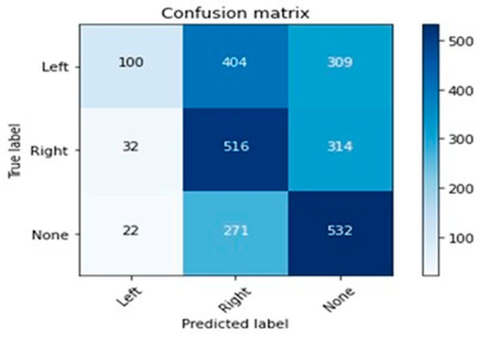
Different classification algorithms, including support vector machine (SVM), decision tree classifier, and random forest classifier, were evaluated for their performance using root-mean-squared error metrics. The results revealed that the initial accuracy achieved using SVM was only 46% (Figure 1), indicating that the model’s performance was limited.

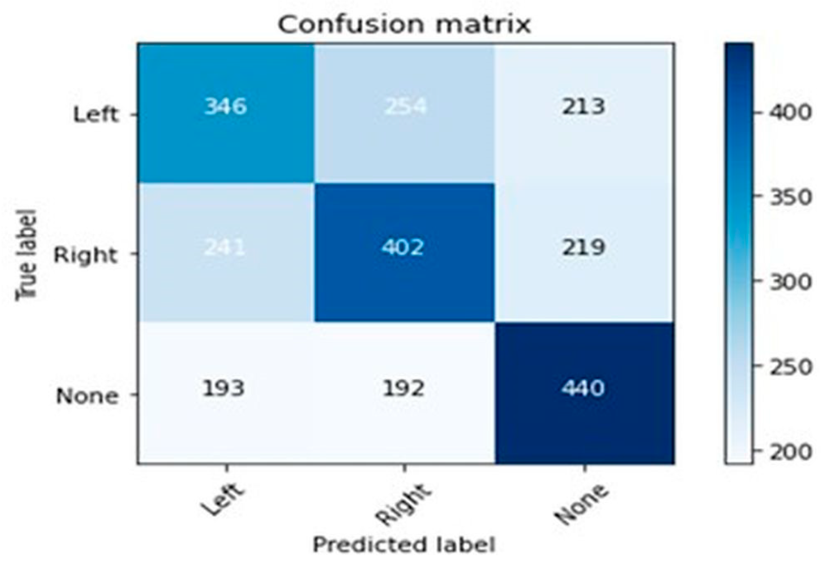
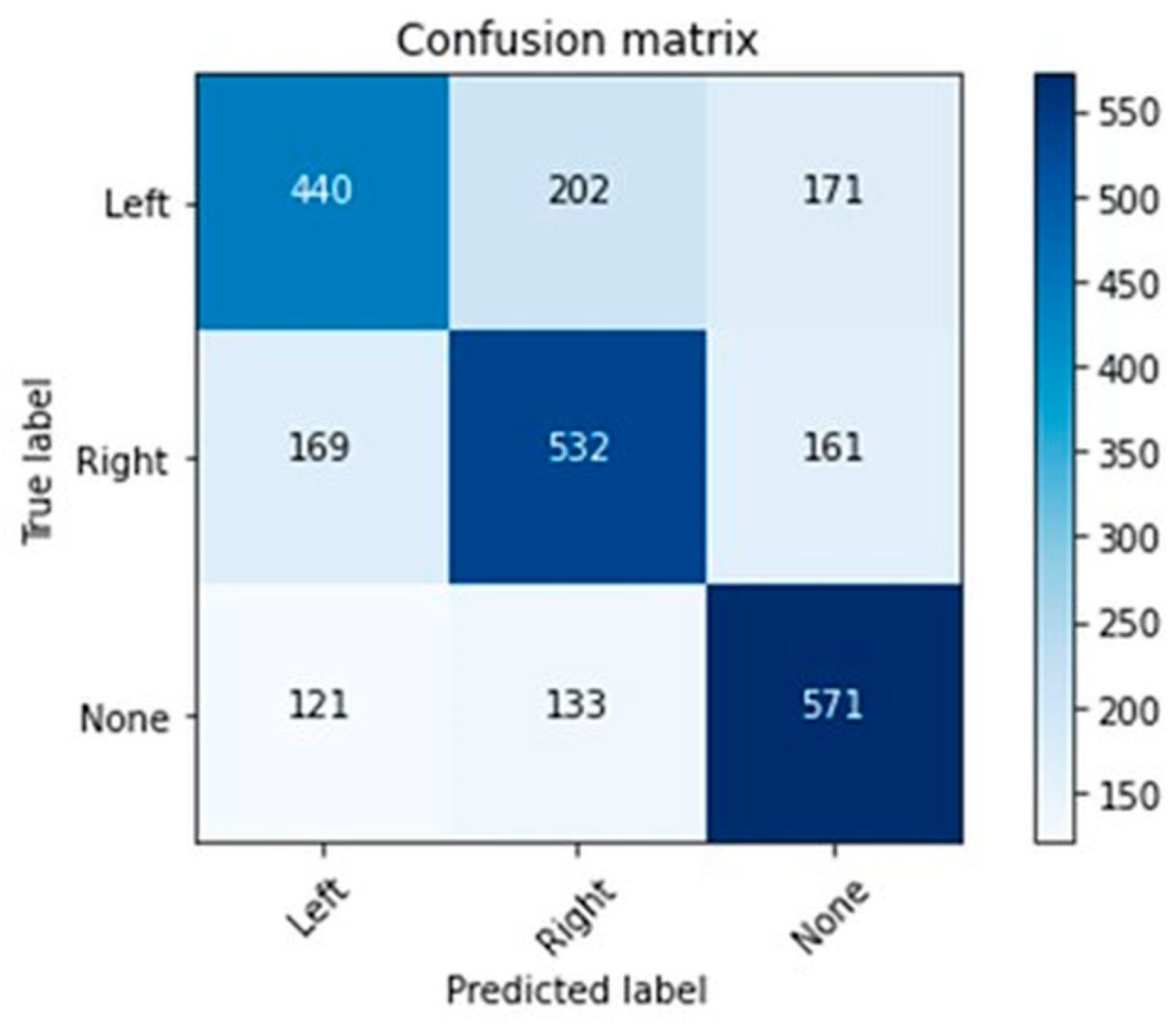
Attempting to enhance the accuracy, the study explored alternative algorithms, such as decision tree classifier and random forest classifier. This effort led to a moderate improvement, with the accuracy increasing to 48% (Figure 2) when using the decision tree classifier and further improving to 62% (Figure 3) when using the random forest classifier. However, these outcomes indicated that the constant features approach might not be sufficient to achieve the desired prediction accuracy.

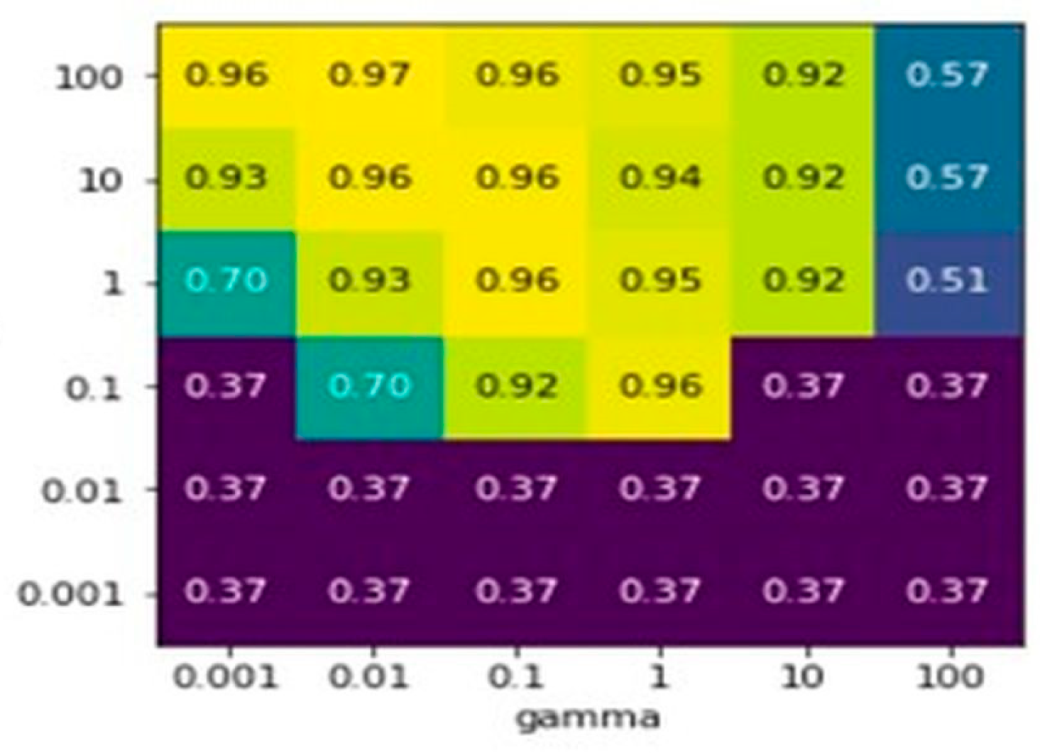
Unfortunately, there were no noticeable improvements to the random forest algorithm in the previous approach with the use of GridSearchCV. The results show only 0.57 accuracy in the precision (Figure 4).

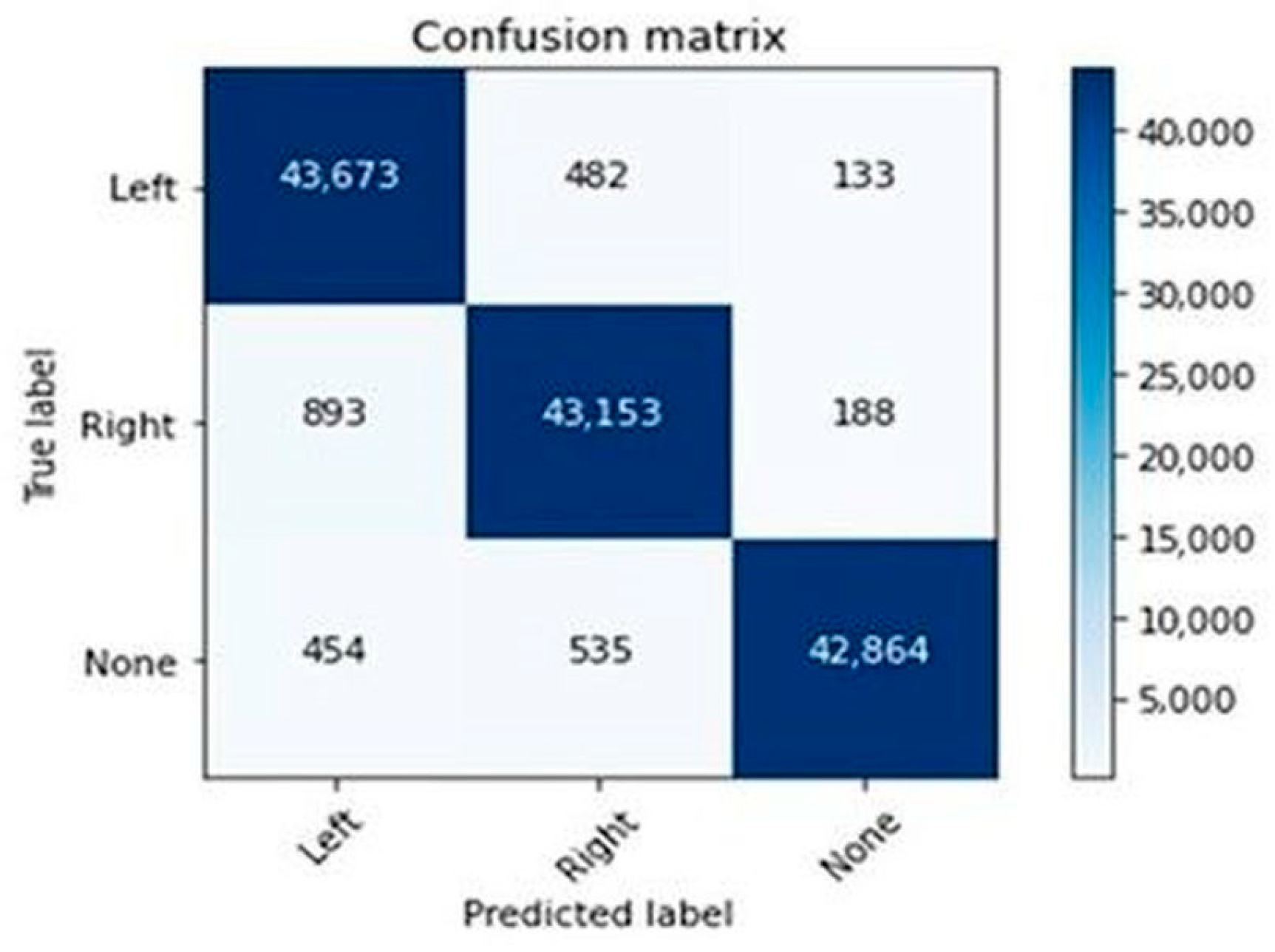
As there were no noticeable improvements to the random forest algorithm of that approach using GridSearchCV, the LSTM confusion matrix (Figure 5) was used.

3.2. Part II: Multivariate Time Series Approach

Given the limitations of the constant features approach, the study then proceeded to Part II, where the focus shifted to the multivariate time series approach. This approach involved a more advanced methodology, employing a neural network architecture consisting of convolutional filters followed by a long short-term memory neural network (LSTM). The convolutional layer’s purpose was to extract high-level features from the EEG data.

The LSTM network, known for its ability to capture long-term dependencies, was employed to overcome the vanishing gradient problem and maintain relevant information over extended sequences. This was particularly well suited for handling the sequential nature of EEG signals. The results obtained from this approach were striking: the model achieved an impressive accuracy of 98% in predicting the chosen action based on EEG signals.

Figure 5 highlights the impact of utilizing the long short-term memory (LSTM) network, known for its proficiency in capturing long-term dependencies within sequential data like EEG signals. LSTM’s capability to overcome challenges like the vanishing gradient problem is crucial, allowing it to retain relevant information over extended sequences—ideal for EEG’s sequential nature. The confusion matrix in Figure 5 offers insight into the LSTM model’s performance. Breaking down predictions against actual labels, it visually represents true positives, true negatives, false positives, and false negatives. Regarding study results, the figure showcases the LSTM’s prowess in classification’s accuracy. High counts of true positives and true negatives affirm its proficiency in identifying action instances. False positives and negatives reveal areas for future improvement. Accuracy metrics within Figure 5 further quantify success, demonstrating the LSTM’s exceptional 98% accuracy in predicting actions from EEG signals. This underscores LSTM’s efficacy in comprehending complex EEG patterns and associating them with actions.

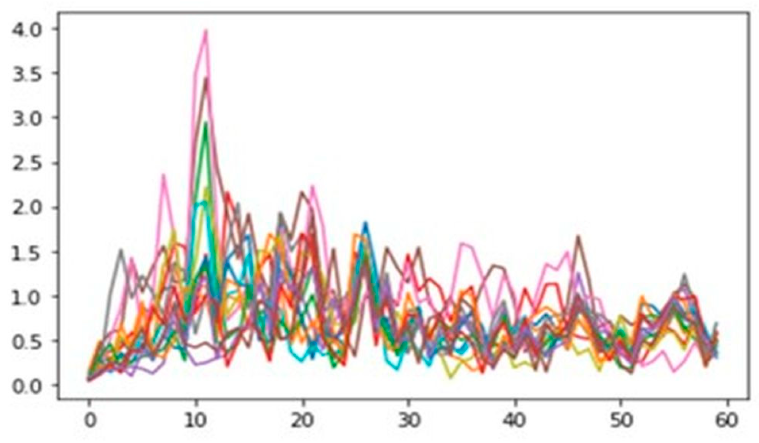
Using a 16-channel extraction (Figure 6), resulted in achieving an accuracy of 98%, thus proving to be the best model for this study. Figure 6, enhanced by the LSTM network, provided in-depth insights. The model’s ability to capture long-term dependencies aligns seamlessly with EEG’s sequential nature. The graph plots frequency (Hz) on the x-axis and amplitude (V) on the y-axis, revealing intricate spectral components from EEG data.

For action prediction from EEG signals, Figure 6 illuminates neural activity patterns linked to different actions. Prevalent spectral components at specific frequencies indicate brainwave frequencies tied to actions. Concentrated components on the left, touching an amplitude of 4, signify lower-frequency neural dominance during these actions. Integrating LSTM’s capabilities emphasizes its effectiveness in unraveling EEG intricacies across actions, reinforcing the key finding of 98% accurate action classification.

4. Discussion

The aim of this study was to predict a chosen action (left) based on EEG signals extracted from the brain using the two headsets for potential usage on robotic arms or devices. Long short-term memory (LSTM) networks were chosen as the method of prediction due to their ability to handle sequential data and maintain information over a longer period. The EEG signals were preprocessed to remove noise and ensure consistency. A deep learning model based on LSTM networks was developed to perform the prediction. The model was trained using a portion of the EEG signals, and its performance was evaluated using a separate test dataset.

The results of the study showed that the LSTM networks outperformed other methods in terms of accuracy, achieving an accuracy of 98% in the prediction task. These results suggested that LSTM networks could effectively handle the sequential nature of EEG signals and provide accurate predictions for the chosen action.

Overall, the ML-based model developed in this study had the potential to control robotic arms or other robotic devices using EEG signals extracted from the brain and may have important applications in the field of brain–computer interfaces.

5. Conclusions

This study demonstrated the effectiveness of using LSTM networks for predicting actions based on EEG signals extracted from the headsets. The results demonstrated a high accuracy of 98%, indicating the potential of this approach for developing brain–computer interfaces. However, the limitations of the Emotiv EPOC and OpenBCI in terms of signal-to-noise ratio and electrode number should be considered when interpreting the results. The Emotiv EPOC and the OpenBCI are consumer-grade brain–computer interfaces that are designed for noninvasive monitoring of brain activity. One of the major limitations of these headsets is their signal-to-noise ratio, which affects the accuracy of the device in detecting and interpreting brain signals. The devices are also limited by their small number of electrodes, which reduces their ability to capture the full spectrum of brain activity and can result in measurement errors. Further research with larger datasets and more advanced EEG recording devices can provide deeper insights into the potential of this approach for real-world applications. Future research could also focus on examining the generalizability of the developed LSTM model to other EEG datasets and brain–computer interface (BCI) devices. This could involve collecting and preprocessing EEG data from different devices and datasets and testing the performance of the model on these new datasets. Assessing the potential for real-world applications is also an important direction for future research. This could involve testing the model in more realistic scenarios, such as in real-time BCI applications or in more complex tasks that require the prediction of multiple actions. Additionally, further investigation into methods for improving the signal-to-noise ratio of the Emotiv EPOC, OpenBCI, or other consumer-grade BCI devices could lead to more accurate predictions and more reliable real-world applications. Finally, it may also be valuable to investigate the interpretability of the model and its ability to provide insights into the underlying brain activity that is associated with the predicted actions. This could involve techniques such as visualization of the learned representations within the LSTM network or feature importance analysis. Such insights could be valuable for understanding the neural mechanisms underlying the chosen action and could inform the development of more effective BCI systems.

References

- Kakkos, I.; Miloulis, S.-T.; Gkiatis, K.; Dimitrakopoulos, G.N.; Matsopoulos, G.K. Human–Machine Interfaces for Motor Rehabilitation. In Advanced Computational Intelligence in Healthcare-7: Biomedical Informatics; Maglogiannis, I., Brahnam, S., Jain, L.C., Eds.; Studies in Computational Intelligence; Springer: Berlin/Heidelberg, Germany, 2020; pp. 1–16. ISBN 978-3-662-61114-2. [Google Scholar]
- Zorzos, I.; Kakkos, I.; Miloulis, S.T.; Anastasiou, A.; Ventouras, E.M.; Matsopoulos, G.K. Applying Neural Networks with Time-Frequency Features for the Detection of Mental Fatigue. Appl. Sci. 2023, 13, 1512. [Google Scholar] [CrossRef]
- Schirrmeister, R.T.; Springenberg, J.T.; Fiederer, L.D.J.; Glasstetter, M.; Eggensperger, K.; Tangermann, M.; Hutter, F.; Burgard, W.; Ball, T. Deep Learning with Convolutional Neural Networks for EEG Decoding and Visualization. Hum. Brain Mapp. 2017, 38, 5391–5420. [Google Scholar] [CrossRef] [PubMed]
- Isa, N.E.M.; Amir, A.; Ilyas, M.Z.; Razalli, M.S. Motor Imagery Classification in Brain Computer Interface (BCI) Based on EEG Signal by Using Machine Learning Technique. Bull. Electr. Eng. Inform. 2019, 8, 269–275. [Google Scholar] [CrossRef]
- Publicly Available EEG Datasets. Available online: https://openbci.com/community/publicly-available-eeg-datasets/ (accessed on 21 February 2021).
- Patrón, J.S.; Monje, C.R.B. Emotiv EPOC BCI with Python on a Raspberry Pi. Sist. Telemát. 2016, 14, 27–38. [Google Scholar] [CrossRef]
- Kakkos, I.; Ventouras, E.M.; Asvestas, P.A.; Karanasiou, I.S.; Matsopoulos, G.K. A Condition-Independent Framework for the Classification of Error-Related Brain Activity. Med. Biol. Eng. Comput. 2020, 58, 573–587. [Google Scholar] [CrossRef] [PubMed]
- Scikit-Learn: Machine Learning in Python. BibSonomy. Available online: https://www.bibsonomy.org/bibtex/2dc85c63c6e5ec01a36a3f383bbdaedf5/l.sz.?lang=de (accessed on 4 February 2021).
- Breiman, L. Random Forests. Mach. Learn. 2001, 45, 5–32. [Google Scholar] [CrossRef]
- Chen, T.; Guestrin, C. XGBoost: A Scalable Tree Boosting System. In Proceedings of the 22nd ACM SIGKDD International Conference on Knowledge Discovery and Data Mining, San Francisco, CA, USA, 13–17 August 2016; Association for Computing Machinery: New York, NY, USA, 2016; pp. 785–794. [Google Scholar]
- Hochreiter, S.; Schmidhuber, J. Long Short-Term Memory. Neural Comput. 1997, 9, 1735–1780. [Google Scholar] [CrossRef] [PubMed]