Proceeding Paper

A Hypothesis Test for the Goodness-of-Fit of the Marginal Distribution of a Time Series with Application to Stablecoin Data †

Department of Computer Science and Information Systems, Birkbeck, University of London, London WC1E 7HX, UK
Presented at the 7th International conference on Time Series and Forecasting, Gran Canaria, Spain, 19–21 July 2021.
Eng. Proc. 2021, 5(1), 10; https://doi.org/10.3390/engproc2021005010
Published: 25 June 2021
(This article belongs to the Proceedings of The 7th International Conference on Time Series and Forecasting)

Abstract

:
A bootstrap-based hypothesis test of the goodness-of-fit for the marginal distribution of a time series is presented. Two metrics, the empirical survival Jensen–Shannon divergence ( E S J S ) and the Kolmogorov–Smirnov two-sample test statistic ( K S 2 ), are compared on four data sets—three stablecoin time series and a Bitcoin time series. We demonstrate that, after applying first-order differencing, all the data sets fit heavy-tailed α -stable distributions with 1 < α < 2 at the 95% confidence level. Moreover, E S J S is more powerful than K S 2 on these data sets, since the widths of the derived confidence intervals for K S 2 are, proportionately, much larger than those of E S J S .

1. Introduction

The empirical survival Jensen–Shannon divergence ( E S J S ) has recently been proposed as a goodness-of-fit measure of a fitted parametric continuous distribution [1]. However, the important issue of hypothesis testing whether the output E S J S value is significant was left open.
To alleviate this problem, we propose a hypothesis test based on the parametric bootstrap [2,3], and evaluate the method on time series data [4,5]. As a proof of concept, we chose four cryptocurrency time series, three stablecoin [6] data sets, and, for reference, we employ a fourth, Bitcoin [7], data set. The stablecoins we chose maintain their “stability” by being pegged to the dollar, and thus one would expect their volatility to be low. Apart from the general interest in cryptocurrency time series, it has already been shown that Bitcoin data are heavy-tailed [8]; thus, demonstrating that stablecoins also exhibit heavy tails is interesting in its own right. One reason to experiment with heavy-tailed distributions, such as the α -stable distribution [9] (or simply the stable distribution) employed herein, is that they pose additional problems compared to, say, the normal distribution (in the special case when α = 2 ) due to their variance being infinite (in the more general case when α < 2 ).
The rest of the paper is organised as follows: In Section 2, we introduce the E S J S and, for comparison purposes, also bring in the well-known Kolmogorov–Smirnov two-sample test statistic ( K S 2 ) [10] Section 6.3. In Section 3, we present a parametric bootstrap-based goodness-of-fit hypothesis test. Time series do not necessarily comprise independent and identically distributed (iid) random variables (as is assumed in, say, [11]), so utilising more general models, such as autoregressive models (as is assumed in, say, [12]), is more appropriate when generating time series bootstrap samples. Here, we assume an autoregressive process of order one [4,5], abbreviated to AR(1), with α -stable innovations, as in [13,14]. In Section 4, we introduce the cryptocurrency time series we experiment with, and fit them to a stable distribution after applying first-order differencing to the raw data, to obtain stationary processes. In particular, we demonstrate that in this case α < 2 , that is, they are not normally distributed. In Section 5, we apply the goodness-of-fit hypothesis test of Section 3 to the cryptocurrency time series described in Section 4 and discuss the results. Finally, in Section 6, we provide our concluding remarks. We note that all computations were carried out using the Matlab software package.

2. Empirical Survival Jensen–Shannon Divergence

To set the scene, we assume a time series, x = { x 1 , x 2 , , x n } , where x t , for t = 1 , 2 , , n is a value indexed by time, t, for example, modelling the movement of a stock price. More specifically, a time series of n values is a random sample generated by a stochastic process that forms a sequence of random variables X = X 1 , X 2 , , X n , where each value x i is a realisation of the random variable X i . The stochastic process X may be a sequence of iids, but, more often than not, a time series exhibits temporal dependencies between its values, which is more realistic. We will also assume that the time series is stationary [4,5]. This makes sense in our context, since we are particularly interested in the marginal distribution of x , which we suppose comes from an underlying parametric continuous distribution D.
The empirical survival function of a value z for the time series x , denoted by S ^ ( x ) [ z ] , is given by
S ^ ( x ) [ z ] = 1 n i = 1 n I { x i > z } ,
where I is the indicator function. In the following, we will let P ^ ( z ) = S ^ ( x ) [ z ] stand for the empirical survival function S ^ ( x ) [ z ] , where the time series x is assumed to be understood from the context; we will generally be interested in the empirical survival function P ^ , which we suppose arises from the survival function P of the parametric continuous distribution D, mentioned above.
The empirical survival Jensen–Shannon divergence ( E S J S ) [1] between two empirical survival functions, Q ^ 1 and Q ^ 2 , arising from the survival functions Q 1 and Q 2 , is given by
E S J S ( Q ^ 1 , Q ^ 2 ) = 1 2 0 Q ^ 1 ( z ) log Q ^ 1 ( z ) M ^ ( z + Q ^ 2 ( z ) log Q ^ 2 ( z ) M ^ ( z ) d z ,
where
M ^ ( z ) = 1 2 Q ^ 1 ( z ) + Q ^ 2 ( z ) .
We note that the E S J S is bounded and can thus be normalised, so it is natural to assume its values are between 0 and 1; in particular, when Q ^ 1 = Q ^ 2 its value is zero. Moreover, its square root is a metric (cf. [1]).
For completeness, we provide the definition of the Kolmogorov–Smirnov two-sample test statistic ([10] Section 6.3) between Q ^ 1 and Q ^ 2 as above, which is given by
K S 2 ( Q ^ 1 , Q ^ 2 ) = m a x z | Q ^ 1 ( z ) Q ^ 2 ( z ) | ,
where m a x is the maximum function, and | v | is the absolute value of a number v. We note that K S 2 is bounded between 0 and 1, and is also a metric.
Now, for a parametric continuous distribution D, we let ϕ = ϕ ( D , P ^ ) be the parameters that are obtained from fitting D to the empirical survival function, P ^ . The distribution D may, in principle, be any continuous distribution, although here we concentrate on the α -stable distribution, since it allows for the modelling of heavy-tailed data, which poses additional problems to those of light-tailed data, due to the variance (and possibly the mean) being infinite. In particular, we have an interest in cryptocurrency data, which is likely to be heavy-tailed [8].
We now let P ϕ = S ϕ ( x ) be the survival function of x , for D with parameters ϕ . Thus, the empirical survival Jensen–Shannon divergence and the Kolmogorov–Smirnov two-sample test statistic, between P ^ and P ϕ , are given by E S J S ( P ^ , P ϕ ) and K S 2 ( P ^ , P ϕ ) , respectively. These values provide us with two measures of goodness-of-fit for how well D, with parameters ϕ , is fitted to x (cf. [1]).

3. A Bootstrap-Based Goodness-of-Fit Hypothesis Test

Our hypothesis test makes use of the parametric bootstrap [2,3]; the pseudocode for the parametric bootstrap in our context is given in Algorithm 1. It takes as input a time series x , the distribution D we hypothesise x comes from, and the number of bootstrap samples m; in the simulations we use the typical value of m = 1000 samples [15]. The algorithm outputs two vectors, B V - E S J S and B V - K S 2 . The first contains m E S J S values, for i = 1 , 2 , , m , between the empirical survival function P ^ i = S ^ ( B i ) for the ith bootstrap sample, B i , and the survival function P ϕ = S ϕ ( x ) of x , for D with parameters ϕ . Correspondingly, the second contains m K S 2 values, for i = 1 , 2 , , m , between P ^ i and P ϕ . The bootstrap samples are generated by an AR(1) process with α -stable distribution innovations [14] (see also [13]), which is more realistic than assuming that the samples are generated from an iid process, as in [11].
Algorithm 1: Parametric-Boostrap( x , D , m ).
 1.   begin
 2.         Initialise B V - E S J S and B V - K S 2 as the vector, 0 , 0 , , 0 , of m zeros;
 3.        Let n be the number of values in x ;
 4.        Let ϕ = ϕ ( D , P ^ ) ;
 5.        Let P ϕ = S ϕ ( x ) ;
 6.        for  i = 1  to m do
 7.          Generate a bootstrap sample B i = x i 1 * , x i 2 * , , x i n * ,
 8.            where B i is generated from an AR(1) process with innovations
                 derived from D with parameters ϕ ;
 9.          Let P i ^ = S ^ ( B i ) ;
 10.          Let B V - E S J S ( i ) = E S J S ( P ^ i , P ϕ ) ;
 11.           Let B V - K S 2 ( i ) = K S 2 ( P ^ i , P ϕ ) ;
 12.        end for
 13.        return  B V - E S J S and B V - K S 2 sorted in ascending order.
 14.   end
As we have assumed that the time series is stationary, the absolute value | ρ | of the parameter ρ of the AR(1) process generating x should be less than one. For the generation process, we use an estimate ρ ^ of ρ , and, as we will see in Section 4, | ρ ^ | < 1 is satisfied for the data sets we employ, as required. We also add a burn-in period of 100 steps to the AR(1) process generated, which we found to be sufficient for the data sets we used.
Given the bootstrap vectors, B V - E S J S and B V - K S 2 , and the output from Algorithm 1, we can form confidence intervals for E S J S ( P ^ , P ϕ ) and K S 2 ( P ^ , P ϕ ) , according to the bootstrap percentile method ([16] Section 3.1.2), which is the simplest way to construct a bootstrap confidence interval; see [16] for improvements on the percentile method. We assume that the significance level we are interested in for a hypothesis test is a percentage, and set the significance level to 5%, which is the value we will use in Section 5.
Subsequently, for a one-sided test, we would exclude the highest 5 % values from the parametric bootstrap vector, say B V , returned from Algorithm 1, and for a two-sided test we would exclude from B V the lowest 2.5 % values and the highest 2.5 % values. For both E S J S and K S 2 only a one-sided test makes sense, since both metrics are bounded below by zero. Therefore, the null hypothesis is that the distribution of P ^ is D, and so we reject the null hypothesis at the 5 % confidence level, if E S J S ( P ^ , P ϕ ) or, correspondingly, K S 2 ( P ^ , P ϕ ) is greater than the upper bound of the constructed confidence interval, depending on which goodness-of-fit measure we are employing.

4. Cryptocurrencies and Heavy Tails

As a proof of concept, we analysed four time series data sets. These include the prices of three stablecoins [6]: Tether (https://tether.to, accessed on 1 June 2021), DAI (https://makerdao.com, accessed on 1 June 2021) and USDC (https://www.centre.io/usdc, accessed on 1 June 2021), which are all pegged to the dollar. In addition, for comparison purposes, we make use of a fourth time series data set, the price of the archetypal decentralised cryptocurrency, Bitcoin [7], the price of which has previously been hypothesised to follow the heavy-tailed stable distribution [8].
In Table 1, we describe the details of the time series data we used for the empirical validation of the proposed goodness-of-fit method; the data were obtained from Coin Metrics (https://coinmetrics.io, accessed on 1 June 2021). For the stablecoins, 1 is subtracted from the daily closing rate, so that its value is positive if above 1, zero if exactly 1, and negative if below 1. For analysis purposes we applied first-order differencing [4,5] to all the time series, that is, we computed the difference between consecutive observations, which is useful for removing trends, transforming the price time series into a return series (in future work we will also consider analysing the raw data set without differencing; however, since our main aim is to introduce the hypothesis test, for brevity and clarity of exposition we will not consider this further analysis here). The time series, after differencing was applied to the raw data sets, are shown in Figure 1.
The α -stable distribution (or simply the stable distribution) [9] has four parameters: (i) the characteristic exponent α ( 0 , 2 ] ; (ii) the skewness parameter β [ 1 , 1 ] (when β = 0 , the distribution is symmetric); (iii) the scale parameter γ ; and (iv) the location parameter δ . It is heavy-tailed unless α = 2 , when the stable distribution reduces to the light-tailed normal distribution with β = 0 . When α < 2 , the stable distribution is heavy-tailed, its variance as well as all its other higher moments are infinite; in the case of α 1 , its mean is also infinite. In the following we will refer to a distribution as stable when α < 2 , and normal when α = 2 .
In Figure 2, we show the histograms of the marginal distributions of the four cryptocurrencies overlaid with the curve of the maximum likelihood fit of the normal distribution to the data. It is visually evident that the normal distribution is not a good fit for these data sets. Kurtosis of a distribution, in this case the marginal distribution of a time series, indicates peakedness and tailedness of the data relative to the normal distribution [17] (for ease of comparison with the kurtosis of the normal distribution, which is 3, we will subtract 3 from the kurtosis, giving the excess kurtosis). In Table 2, we show the excess kurtosis of the four cryptocurrencies, which provides further evidence that none of them follow a normal distribution, and are in fact heavy-tailed.
Next, we fitted the stable distribution to the four data sets using the Matlab implementation provided by [18], which is based on the empirical characteristic function method [19]. The fitted parameters are shown in Table 3, noting that in all cases 1 < α < 2 , implying that the means of the marginal distributions are finite but their variances are infinite.

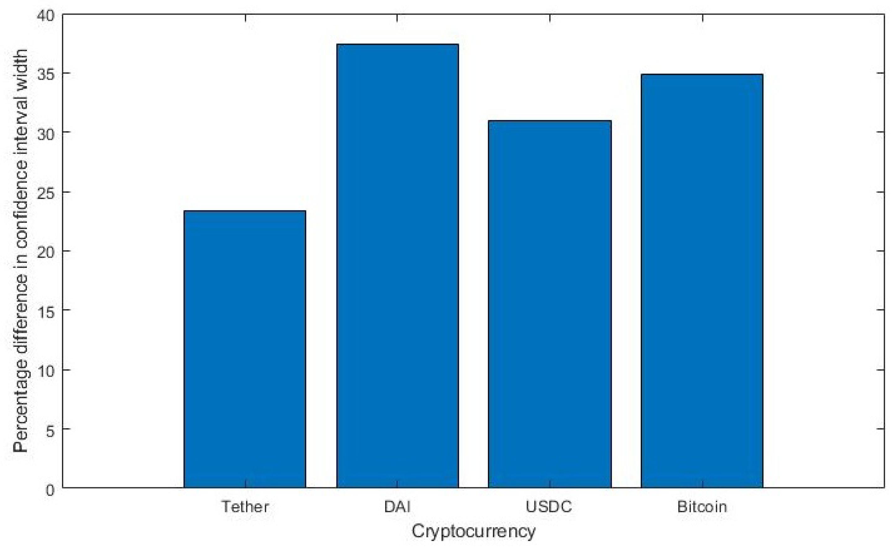
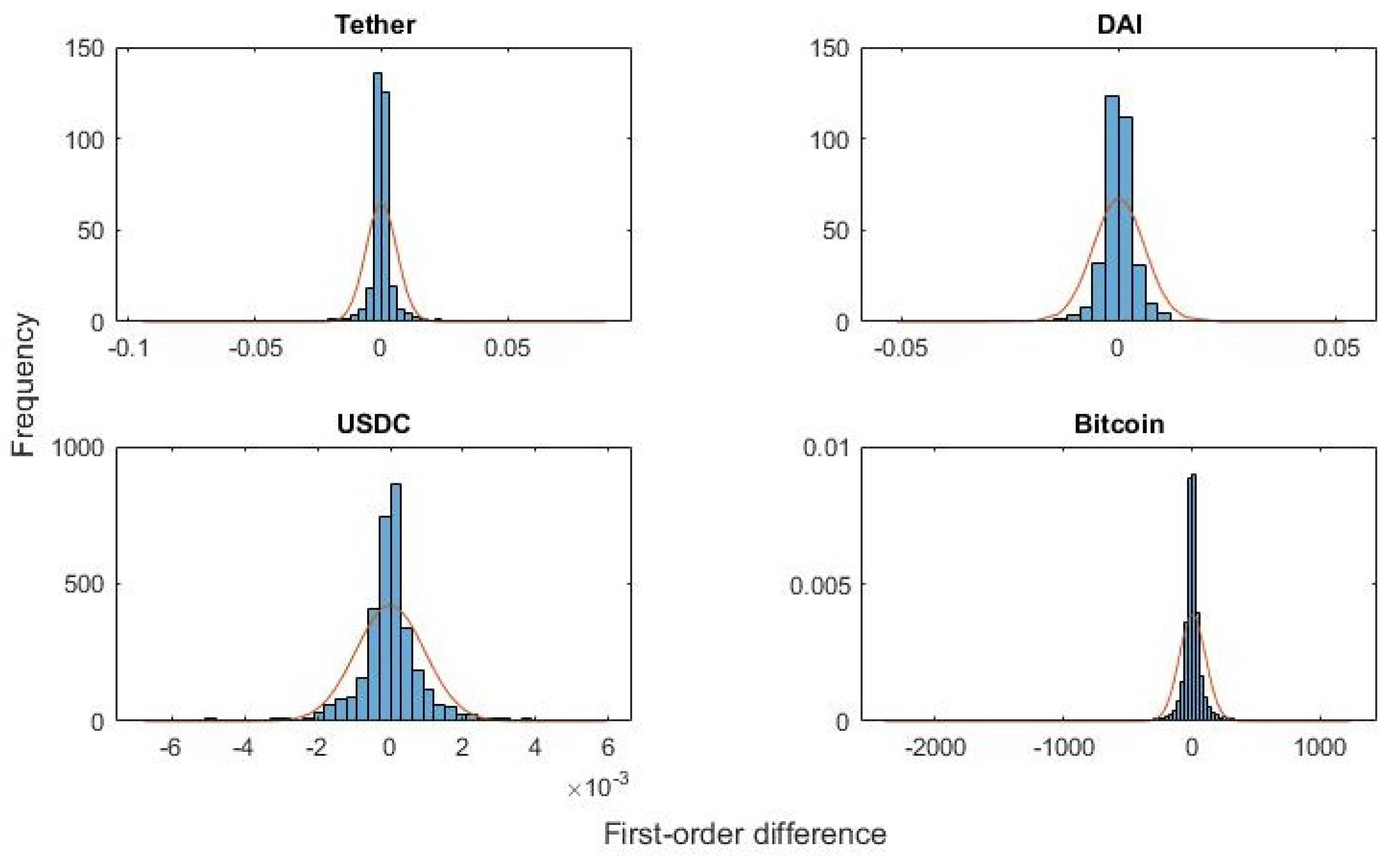
5. Application of the Goodness-Of-Fit Hypothesis Test to Cryptocurrencies

We apply the bootstrap goodness-of-fit test presented in Section 3, based on the empirical survival Jensen–Shannon divergence ( E S J S ) and Kolmogorov–Smirnov two-sample test statistic ( K S 2 ) metrics, to construct 95% confidence intervals for E S J S ( P ^ , P ϕ ) and K S 2 ( P ^ , P ϕ ) , where P ^ is the empirical survival function of the input time series and P ϕ is the survival function of time series x , for D with parameters ϕ . When running Algorithm 1, we computed 1000 bootstrap samples, that is, we set m = 1000 . Moreover, it can be seen in Table 4 that, for all data sets, the estimate ρ ^ of the AR(1) parameter is less than one in absolute value, implying that the generated bootstrap time series, B i , are stationary as required.
In Table 5 and Table 6, we show the results of the bootstrap hypothesis test when employing the E S J S and K S 2 metrics, respectively. In particular, for all data sets, both metrics are within the 95% confidence interval, and thus with 95% confidence we cannot reject the null hypothesis that the marginal distribution of the input time series comes from an α -stable distribution.
The bar chart in Figure 3 shows that for all four cryptocurrencies the width of the confidence interval for the K S 2 goodness-of-fit measure is, proportionately, much larger than that of the E S J S goodness-of-fit measure. Statistical tests using measures resulting in smaller confidence intervals are normally considered to be more powerful as this implies, with high confidence, that a smaller sample size may be deployed [20].
Finally, to provide contrast to the stable distribution result, we now hypothesise that the marginal distribution of the time series is actually normal (i.e., α = 2 ). We see in Table 7 that, for all four cryptocurrencies, we reject the null hypothesis that the marginal distribution is normal, as both the E S J S and K S 2 are outside their respective 95% confidence intervals.

6. Concluding Remarks

We presented a proof of concept of the bootstrap-based goodness-of-fit test on four cryptocurrency time series, concentrating on the α -stable distribution, which allows for the modelling of heavy-tailed data. Our results demonstrate that, when first-order differenced, the marginal distributions of all four time series are all α -stable with α < 2 . Moreover, for both E S J S and K S 2 , the confidence level of the bootstrap-based test is at the 95% level. Furthermore, E S J S is more powerful than K S 2 on these data sets, since the widths of the derived confidence intervals for the K S 2 measure are, proportionately, much larger than those for the E S J S measure.
We emphasise that the proposed goodness-of-fit test may be applied to any marginal distribution, not just to the heavy-tailed stable distributions. Thus, there is a need to further establish the validity of the proposed hypothesis test on more data sets and on a variety of distributions, which may or may not be heavy-tailed. In addition, it would be useful to look at the assumptions regarding the process underlying the generation of the time series, and to ascertain how this affects the hypothesis test.

References

  1. Levene, M.; Kononovicius, A. Empirical survival Jensen–Shannon divergence as a goodness-of-fit measure for maximum likelihood estimation and curve fitting. Commun. Stat.-Simul. Comput. 2019. [Google Scholar] [CrossRef] [Green Version]
  2. Ventura, V. Bootstrap Tests of Hypotheses. In Analysis of Parallel Spike Trains; Springer Series in Computational Neuroscience; Grün, S., Rotter, S., Eds.; Springer: Boston, MA, USA, 2010; Volume 7, Chapter 18; pp. 383–398. [Google Scholar]
  3. Pewsey, A. Parametric bootstrap edf-based goodness-of-fit testing for sinh–arcsinh distributions. TEST 2018, 27, 147–172. [Google Scholar] [CrossRef]
  4. Enders, W. Applied Econometric Time Series, 4th ed.; Wiley Series in Probability and Statistics; John Wiley & Sons: Hoboken, NJ, USA, 2014. [Google Scholar]
  5. Chatfield, C.; Xing, H. The Analysis of Time Series: An Introduction with R, 7th ed.; Text in Statistical Science; Chapman & Hall: London, UK, 2019. [Google Scholar]
  6. Sidorenko, E. Stablecoin as a new financial instrument. In Proceedings of International Scientific Conference on Digital Transformation of the Economy: Challenges, Trends, New Opportunities; Springer Nature: Cham, Switzerland, 2020. [Google Scholar]
  7. Judmayer, A.; Stifter, N.; Krombholz, K.; Weippl, E.; Bertino, E.; Sandhu, R. Blocks and Chains: Introduction to Bitcoin, Cryptocurrencies, and Their Consensus Mechanisms; Synthesis Lectures on Information Security; Privacy, and Trust, Morgan & Claypool Publishers: San Francisco, CA, USA, 2017. [Google Scholar]
  8. Kakinaka, S.; Umeno, K. Characterizing cryptocurrency market with Lévy’s stable distributions. J. Phys. Soc. Jpn. 2020, 89, 024802-1–024802-13. [Google Scholar] [CrossRef] [Green Version]
  9. Nolan, J. Univariate Stable Distributions: Models for Heavy Tailed Data; Springer Series in Operations Research and Financial Engineering; Springer Nature: Cham, Switzerland, 2020. [Google Scholar]
  10. Gibbons, J.; Chakraborti, S. Nonparametric Statistical Inference, 6th ed.; Marcel Dekker: New York, NY, USA, 2021. [Google Scholar]
  11. Cornea-Madeira, A.; Davidson, R. A parametric bootstrap for heavy-tailed distributions. Econom. Theory 2015, 31, 449–470. [Google Scholar] [CrossRef] [Green Version]
  12. Lin, J.; McLeod, A. Improved Peňa–Rodriguez portmanteau test. Comput. Stat. Data Anal. 2006, 51, 1731–1738. [Google Scholar] [CrossRef]
  13. Gallagher, C. A method for fitting stable autoregressive models using the autocovariation function. Stat. Probab. Lett. 2001, 53, 381–390. [Google Scholar] [CrossRef]
  14. Ouadjed, H.; Mami, T. Estimating the tail conditional expectation of Walmart stock data. Croat. Oper. Res. Rev. 2020, 11, 95–106. [Google Scholar] [CrossRef]
  15. Hesterberg, T. what teachers should know about the bootstrap: Resampling in the undergraduate statistics curriculum. Am. Stat. 2015, 69, 371–386. [Google Scholar] [CrossRef] [PubMed] [Green Version]
  16. Chernick, M. Bootstrap Methods: A Guide for Practitioners and Researchers, 2nd ed.; Wiley Series in Probability and Statistics; John Wiley & Sons: Hoboken, NJ, USA, 2008. [Google Scholar]
  17. DeCarlo, L. On the meaning and use of kurtosis. Psychol. Methods 1997, 2, 292–307. [Google Scholar] [CrossRef]
  18. Veillette, M. Alpha-Stable Distributions in MATLAB. 2015. Available online: http://math.bu.edu/people/mveillet/html/alphastablepub.html (accessed on 1 June 2021).
  19. Koutrouvelis, I. An iterative procedure for the estimation of the parameters of stable laws. Commun. Stat.-Simul. Comput. 1981, 10, 17–28. [Google Scholar] [CrossRef]
  20. Liu, X. Comparing sample size requirements for significance tests and confidence intervals. Couns. Outcome Res. Eval. 2013, 4, 3–12. [Google Scholar] [CrossRef]
Figure 1. The time series of the four cryptocurrencies after differencing was applied to the raw data sets.
Engproc 05 00010 g001
Figure 2. Histograms of the marginal distributions of the four cryptocurrencies, each overlaid with the curve of the maximum likelihood fit of the normal distribution to the data.
Engproc 05 00010 g002
Figure 3. How much larger, proportionately, is the width of the K S 2 confidence interval compared to that of the E S J S ?
Engproc 05 00010 g003
Table 1. Description of time series data used for experimentation; #Values is the number of values in the time series.
Currency#ValuesFromUntilClosing Rate
Tether126406 January 201715 November 2020daily
DAI36220 November 201915 November 2020daily
USDC77228 September 201815 November 2020daily
Bitcoin892901 January 202007 January 2021hourly
Table 2. Excess kurtosis of the four cryptocurrencies.
CurrencyExcess Kurtosis
Tether86.0207
DAI34.6573
USDC10.1905
Bitcoin59.7350
Table 3. Parameters from fits of the stable distribution to the data of the four cryptocurrencies.
Fitted Parameters for Stable Distribution
Currency α β γ δ
Tether1.01110.00190.00110.0001
DAI1.19530.08210.00160.0003
USDC1.22590.01250.00030.0000
Bitcoin1.22610.090927.96857.3644
Table 4. Estimates ρ ^ of the parameter ρ of the AR(1) process for the four cryptocurrencies, noting that, when | ρ | < 1 , the process is stationary.
Currency ρ ^
Tether−0.3604
DAI−0.4045
USDC−0.4948
Bitcoin−0.0504
Table 5. Parametric bootstrap results for the E S J S hypothesis test assuming the marginal distribution is stable; LB, UB, CI, Mean and STD stand for lower bound, upper bound, confidence interval, mean of samples and standard deviation of samples, respectively.
Parametric Bootstrap for E SJS Assuming a Stable Distribution
CurrencyLB of CIUB of CIWidth of CI E S J S MeanSTD
Tether0.00060.02320.02260.00900.01980.0741
DAI0.00300.03450.03150.01560.01880.0096
USDC0.00130.02470.02340.01190.01330.0063
Bitcoin0.00040.00660.00620.00610.00360.0016
Table 6. Parametric bootstrap results for the K S 2 hypothesis test assuming the marginal distribution is stable; LB, UB, CI, Mean and STD stand for lower bound, upper bound, confidence interval, mean of samples and standard deviation of samples, respectively.
Parametric Bootstrap for KS 2 Assuming a Stable Distribution
CurrencyLB of CIUB of CIWidth of CI K S 2 MeanSTD
Tether0.00140.03080.02940.01390.02890.0996
DAI0.00290.05320.05030.03580.02990.0136
USDC0.00350.03740.03390.02190.02100.0093
Bitcoin0.00080.01030.00950.00880.00570.0025
Table 7. Parametric bootstrap results for the E S J S and K S 2 hypothesis tests assuming the marginal distribution of the time series for the four cryptocurrencies is normal; LB and UB stand for lower and upper bounds of the confidence intervals, respectively, and we abbreviate E S J S to E and K S 2 to K.
Parametric Bootstrap Results Assuming a Normal Distribution
CurrencyLB- E UB- E E S J S LB-KUB-K K S 2
Tether0.00010.01320.14400.00040.01820.2162
DAI0.00030.02400.11600.00060.03300.1665
USDC0.00020.01470.08300.00020.02270.1330
Bitcoin0.00010.00670.12180.00000.00850.1708
Publisher’s Note: MDPI stays neutral with regard to jurisdictional claims in published maps and institutional affiliations.

