Abstract
As a small and open economy, Uruguay is highly exposed to international and regional shocks that affect domestic uncertainty. To account for this uncertainty, we construct two geometric uncertainty indices (based on the survey of industrial expectations about the economy and the export market) and explore their association with the Uruguayan GDP cycle between 1998 and 2022. Based on the estimated linear ARDL models that showed negative but weak relationships between the uncertainty indices and the GDP cycle, we test for the existence of structural breaks in these relationships. Although we find a significant break in 2003 for both indices and another in 2019 for one of them, Wald tests performed on the non-linear models only confirm the structural break in the early 2000s in the model with the index based on export market expectations. In this non-linear model, we find that the negative influence of uncertainty fades after 2003. The evidence of a differential influence before and after this date remains, even when controlling for the variability in non-tradable domestic prices. Two implications arise from these results. First, the evidence of relevant changes that made the Uruguayan economy less vulnerable from 2003 onward. Second, the importance of the expectation about the future of the export market in the macroeconomic cycle of a small and open economy like Uruguay.
Keywords:
uncertainty; macroeconomic cycle; expectations; Uruguay; structural breaks; ARDL models; non-linear models JEL Classification:
C53; E32; E37; E71
1. Introduction
A recent and growing trend in the literature that seeks to understand the fundamentals that explain the movements of macroeconomic variables has focused on uncertainty as a relevant factor. Intuitively, economic agents making decisions may not have complete information or the capacity to correctly process the information they possess. This can lead to decisions being made under uncertainty. Moreover, the 2008 global financial crisis made the importance of quantifying uncertainty and having indicators that measure its impact in real-time to detect early signs of the economic situation and contribute to timely decision-making even more evident [1].
However, uncertainty is not a directly measurable phenomenon. Therefore, the economic literature has developed different strategies to capture agents’ uncertainty. Many of the strategies are based on the assumption that prediction errors increase when the uncertainty rises, stock markets become more volatile and the expectations of different economic agents are significantly divergent. Several studies measure uncertainty through the magnitude of forecast errors or by developing dispersion-based indicators of expectations [2,3,4,5]. More recent techniques, based on machine learning, developed new indicators constructed through text analysis ([6,7,8]; among others), including some indicators based on news through processes that could involve some subjectivity [2].
A recent branch of the empirical literature considers survey-based measures of uncertainty. This approach relies on the fact that, in periods of higher uncertainty, there are more discrepancies between the forecasts experts or managers [9,10,11]. This underpins the construction of uncertainty indicators that exploit the dispersion or divergence between agents’ expectations or forecasts. The underlying hypothesis is that lack of predictability and large divergence between forecasters and managers are signs of increased economic uncertainty, and this type of measure captures the uncertainty of decision-makers, who play an important role in investment and innovation decisions. Some empirical applications of this kind of uncertainty indices for macroeconomic forecast are, among others [12,13].
Empirical research on this topic refers mostly to developed economies. However, previous studies, such as [14], found substantial heterogeneity in reactions to uncertainty shocks across countries using an open-economy VAR approach. Compared to developed countries, emerging economies took a longer time to recover, and they relate this effect to the depth of financial markets. Evidence from emerging economies is still scarce (see [15]).
With the aim of contributing to the empirical literature on developing economies, we computed a survey-based uncertainty index for Uruguay following the methodology proposed by [2]. The authors, noting that most survey-based uncertainty indicators do not take into account the responses of agents who do not expect changes in the future [16], propose a time-varying disagreement metric that incorporates information from the three categories of responses. Thus, they construct a positional indicator of disagreement that can be interpreted as the percentage of disagreement between responses. A recent application of this index [17] examines the uncertainty impact on unemployment in European countries one year after the emergence of COVID-19, using two indicators that exploit the European Commission’s survey of business expectations.
The Uruguayan economy has certain characteristics. First, it is a small and open economy located in South America between two large, highly volatile economies, Argentina and Brazil, with which it forms Mercosur. For this economy, the dynamic and influence of uncertainty on the economy are studied in [18,19], using different methods and measures. Ref. [18] proposed a composite index measure of macroeconomic uncertainty that, following the methodology of [20], combines external uncertainty captured by Brazil’s Economic Political Uncertainty (EPU) index (Fundação Getúlio Vargas) and the Global index (Baker, Bloom, and Davis), with domestic uncertainty measured as the standard deviation of 12-month exchange rate forecasts collected by the Central Bank of Uruguay (BCU). On the other hand, Ref. [19] analyze the dynamics of manufacturing firms’ expectations from a network approach, finding that higher uncertainty affects the coordination of groups of firms.
In contrast to the previous studies, this paper considers an alternative uncertainty index for Uruguay, based on economic trend surveys. Following the proposal of [2], we use the industrial monthly survey since 1998, obtained by the Uruguayan Chamber of Industry. We focus on agents’ expectations about the country’s situation in relation to the economy as a whole, both at present and at the end of the next six months. This survey covers 170 companies and asks about expectations for the next 6 months in relation to sales in the domestic market, sales in the foreign market (if applicable), and their expectations for the sector, the company, and the economy. The answer options are: worse, same, better, and don’t know. We explore the relationship between the Uruguayan GDP cycle and uncertainty indices by applying linear and nonlinear models and structural breaks tests. This empirical strategy is in line with that proposed by recent research analyzing how economic uncertainty affects the economy in the short run ([13,21,22], among others).
The rest of the paper is organized as follows. Section 2 presents the data and methodology for the empirical analysis, introducing the uncertainty index for Uruguay based on this methodology. Section 3 presents the empirical results, and the final section, the main conclusions, and policy implications.
2. Data and Methodology
2.1. Data
For the proposed analysis, this article relies mainly on three different sources of information. First, the data used to construct uncertainty indices come from a monthly survey conducted by the CIU. This survey was created in 1997 and one of its objectives is to monitor firms in the manufacturing industry regarding the evolution of different variables. The potential responses were “better, worse, the same (or doesn’t know)”. These responses are later recorded as 1, −1, and 0, respectively. The questions refer to industrialists’ perceptions of the following: (1) The evolution of the national economy in the next six months; (2) If the respondent firm exports, it is asked whether the physical units exported will increase, decrease, or remain the same. Companies are also asked about (3) the evolution of their own sector and (4) the evolution of the company’s domestic sales.
The sample used in this survey contained approximately 200 firms and was first constructed using as a benchmark a different sample designed by the INE. The sample is dynamic [23] in the sense that firms may enter or leave for different reasons, such as the closure of a firm or the entry into the market of a new relevant firm. By means of an analysis carried out by CIU, it is possible to state that the sample is representative of the manufacturing industry. This database contains monthly observations from October 1998 to August 2022, totaling 287 observations.
The change in the percentage of responses to the question regarding the evolution of the economy (question 1) and the evolution of the volume exported in the next six months (question 2) can be seen in Figure A1 and Figure A2, respectively, in the Appendix A.
It can be seen that, for both questions, most companies tend to answer “the same” and that the “worse” answers are, on average, higher than the “better” answers, revealing a certain lack of optimism among companies. There is also a similar evolution of the different response options between the two questions, although differences in level are evident.
Second, the cycle of the Uruguayan economy is extracted from GDP data from Uruguayan Central Bank (BCU). To obtain the cycle, we used the Structural Time Series Analyser, Modeller and Predictor (STAMP) econometric software [24], based on quarterly data from the second quarter of 1980 to the third quarter of 2022. The estimation was performed using the logarithm of the Uruguayan GDP with the following selected options in STAMP: level selected as fixed, the slope as stochastic, the seasonal as stochastic, and an irregular component. The estimated cycle is a short cycle; an intervention analysis was introduced and the estimation method used was maximum likelihood via the BFGS numerical score algorithm.
The estimation for the cycle and the other unobserved components can be seen in Figure A3. The resulting reduction in variance in both the seasonal and the cycle components towards the observations of the latter is noteworthy. Further statistics and results from this estimation can be seen in Table A1.
Finally, in order to consider a factor linked to the domestic market, we also used the year-on-year rate of non-tradable price index (NTP), constructed updating the methodology proposed by [25]. The evolution of the non-tradable inflation can be seen in Figure A4.
2.2. Methodology
This subsection presents the methodology used to compute the uncertainty indexes, based on the aforementioned industrial survey, and to test the existence of a relationship between the economic cycle and the uncertainty index.
2.2.1. Uncertainty Indexes
To construct our geometric uncertainty index we follow [2]. This index is based on the discrepancy of responses to surveys where the answers are (or can be coded as) qualitative. The index also includes respondents that think the variables will remain stable or will not change. The indicator is calculated as follows:
where denotes the share of respondents that answer that the variable will rise in the next period, while is the share that answer will remain constant, the share that considers that will fall and k refers to questions 1 and 2 (the Index constructed with question 1 will now be referred to as Economic Uncertainty, while the one constructed with question 2 will be referred to as Export Uncertainty), which were used to construct the geometric discrepancy index. (an analysis was also conducted for questions 3 and 4, but no significant results were found.) The highest level achievable of uncertainty is reached when the share of responses is equal, i.e., when one-third of the respondents think the variable will rise, one-third think it will remain constant and the last third think it will fall. The evolution of both uncertainty indexes is shown in Figure 1, annotated with the main international and national events in the period.
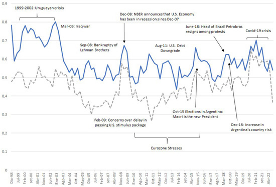
Figure 1.
Geometric Uncertainty Indexes (own calculations based con CIU data). Note: Export Uncertainty Index in blue line, the Economic Uncertainty Index in dotted line.
In the case of economic uncertainty, the mean of the index for the entire period is 0.45, showing two major spikes in 2008 and 2020, which are likely to be related to the financial crisis in 2008 and the appearance of the COVID-19 pandemic. The index related to export uncertainty shows a mean of 0.58, indicating higher levels of expectations misalignment on average, in comparison with the economic uncertainty index. Furthermore, the export uncertainty index does not peak in 2008 and 2020, but rather in 2002, from when a drop in misalignment is evidenced. On the one hand, it is interesting that the indexes present different evolutions because this can have a direct impact on how they relate to the GDP cycle. On the other hand, changes in their own evolution during the period may also suggest that the association with the economic cycle is not constant.
Both of the indexes are I(0), and details of the test [26,27] can be seen in Table A2 in the Appendix A.
2.2.2. Modeling the Link between the Macroeconomic Cycle and Uncertainty
Our first strategy is to estimate an autoregressive distributed lag (ARDL) model, where the economic cycle enters as the dependent variable and the uncertainty index is used as a regressor. This model can be represented as:
where is the value of the economic cycle at time t, k refers to the Index 1 or 2, is the uncertainty index at time t and is supposed to be white noise.
No constant was introduced as the mean of the economic cycle is null by definition. The amount of lags introduced in the model was selected using the Akaike information criterion (AIC). The coefficient covariance matrix used was HAC with the Bartlett Kernel and Newey–West Fixed Bandwith methods.
Then, we tested the existence of structural breaks using the methodology proposed by [28]. Basically, the method consists of considering all the possible partitions given m pre-established breaks and h minimum observations per sub-sample. Then, the sum squared of residuals (SSR) is computed for each partition, looking for the partition where it is minimized. In this article, we first employed a contrast to test the hypothesis of the non-existence of breaks versus the existence of a fixed number of breaks. Secondly, we performed and presented the test of l breaks versus breaks to test whether the breaks are significantly different from each other. It is worth noting that, as the model utilized in Equation (2) is multivariate, the tests described previously admit structural breaks at all parameters.
Finally, if we find significant breaks in the relationship between uncertainty and the GDP cycle, we will proceed to estimate a new specification that takes this into account. Specifically, the objective is to evidence the existence of possible changes in the dynamics of the association between both series.
3. Results
This section presents the results obtained from the different estimations that were performed. The section is divided into three parts: (i) linear bivariate estimation and break search; (ii) bivariate estimation with breaks; and (iii) estimation incorporating the price index of non-tradable goods and services as a control.
3.1. Linear Bivariate Association
Table 1 and Table 2 present the results of the ARDL estimation of the relationship between the GDP cycle and the economic and export uncertainty indices, respectively. As can be seen, the estimation reveals a relationship with an autoregressive component; at the same time, the contemporaneous coefficient and the first lag of the uncertainty index are also significant. However, the coefficients themselves, beyond the best modeling found, are only significant in the case of economic uncertainty. In fact, a negative relationship is found, i.e., higher levels of misalignment between economic expectations are associated with lower levels in the GDP cycle. Although not statistically significant, this association was also found in the model with foreign market expectations.

Table 1.
ARDL model with Index 1 (own estimations).
Table 2.
ARDL model with Index 2 (own estimations).
However, Uruguay, during the period of analysis, experienced important economic events (crisis in 2002, institutional and government changes, and price shocks, among others); therefore, it may make sense that the association between the series in question has not remained constant. In fact, if we look at the mean and standard deviation in the correlation between the series partitioning the sample in five-year periods, an indication of this may be evident (Table A3).
As mentioned, given the possibility that the association is not constant, we tested for the possible existence of breaks. The results for the Bai and Perron sequential L vs. L+1 test about the presence of significantly different structural breaks in our models are presented in Table 3.
Table 3.
Bai and Perron sequential tests for the existence of structural breaks (own estimations).
Indeed, structural breaks are found in the relationship between the variables. Table 3 shows that for the first model, there are two breaks—in 2003Q2 and 2019Q2—while in the second there is only one break, in 2003Q1. The first break is directly linked to the economic crisis experienced by the country during 2002–2003. In the case of 2019, the break may be linked to a slowdown in the GDP growth rate, accompanied by the subsequent fall caused by the COVID pandemic. The next subsection presents the estimation of the model, incorporating the nonlinearity given by the breaks that were found.
3.2. Non-Linear Bivariate Association
Given the presence of significative break dates and using the ARDL models estimated previously, we incorporate the resulting partitions as interactions. Then, a new specification for the economic uncertainty index can be written as:
where y and are the same variables as in Equation (2), is a dummy variable equal to 1 when the date is between [2003Q3, 2019Q2] and is another dummy equal to 1 when the observation is in [2019Q3, 2022Q3]. Similarly, the specification for the export uncertainty index can be written as:
where is a dummy variable equal to 1 when the dates are between [2003Q2,2022Q3].
In both new specifications it is interesting to see if, in addition to finding a significant relationship, the association between uncertainty and the GDP cycle is significantly different between the periods established by the breaks.
Table 4 shows the results of the model estimation (3). In this model, unlike what was found in the ARDL estimation, only the autoregressive component is significant. The GDP cycle presents a strong inertial factor in its dynamics. Uncertainty regarding the future state of the economy does not seem to be related to the economic cycle, as the coefficients are not significant. Although they are significant in the second period, the Wald test of the joint significance of the coefficients does not allow for us to reject the hypothesis that the sum is 0. The results of this Wald tests can be seen in Table 5.
Table 4.
Results for model with economic uncertainty incorporating structural breaks.
Table 5.
Wald test coefficient restrictions for model with economic uncertainty.
In turn, Table 6, which shows the results regarding uncertainty in international trade, shows interesting results. There is a negative and significant association between this uncertainty index and the GDP cycle; this is only found for the first period. This seems to evidence a possible reduction in the negative effect of uncoordinated expectations on the business cycle. After the economic crisis of 2002–2003, uncertainty regarding international trade does not seem to be significantly associated with the GDP cycle. As in the previous model, the Wald Tests of joint significance are presented in Table 7.
Table 6.
Results for model with Index 2 incorporating structural breaks (own estimations).
Table 7.
Wald test coefficient restrictions for model with export uncertainty.
If we look at the Figure 1 and Figure A3, corresponding to the uncertainty index and the GDP cycle, it is possible to observe two marked trends after the fall: (i) an important reduction in the level of uncertainty, shown by an increase in the share of firms that respond that the expectation regarding exports is that it will remain “the same”; and (ii) a reduction in the variability of the economic cycle.
Among the factors that may be behind these results, it is possible to consider that in a small and open country like Uruguay, the short-term dynamics of GDP (which is what we are observing more clearly when using the cycle) are more relevant to foreign market conditions than to the domestic economy itself. This is mainly because uncertainty regarding possible changes in international markets can be transferred more quickly to GDP.
This significant relationship is relevant for understanding how uncoordinated expectations (in this case, from the industrial sector) affect GDP dynamics. However, it is possible that other factors are also relevant both to the dynamics of the economy and as a channel through which uncertainty is transferred to GDP.
Therefore, in the next section, we re-analyze the relationship between the series, incorporating a non-tradable price index in the estimations. By including this series in the analysis, we seek to control for a possible price effect of goods and services not associated with the foreign market.
3.3. Controlling for Variability in Domestic Prices
Following the steps of the previous subsections, first, an ARDL model is estimated to establish the relevant components in the linear relationship (the non-tradable price index was included in its seasonal difference, i.e., the year-on-year rate of non-tradable inflation).
As can be seen in Table 8 and Table 9 the relevance of the autoregressive component is again evident; all three lags are significant for both models. Uncertainty maintains its significance, even with the inclusion of the non-tradable price index. Moreover, unlike the bivariate ARDL of the first subsection, the export uncertainty index now has a negative and significant association at 10%. Although, in both cases, the relationship between expectations misalignment and the business cycle seems to be negative, the difference found between the models is that, in the case of the economic uncertainty index, the first lag in the variable also appears to be relevant (something not found for the other model). In contrast, the NTP index seems to be positively associated with the cycle.
Table 8.
ARDL model with economic uncertainty and non-tradable price index as regressors (own estimations).
Table 9.
ARDL model with export uncertainty and non-tradable price index as regressors (own estimations).
Subsequently, we analyzed the possible existence of structural breaks. Given the number of observations available (also reduced by the inclusion of the seasonal difference of the NTP Index), we established in the break tests that only a maximum of two breaks can be found. If this restriction is not established, a third structural break is found in 2012Q3, and in 2007Q2 for the economic uncertainty model and export uncertainty model, respectively. As can be seen in Table 10, the breaks that were found are extremely similar to those found in Section 3.1: one linked to the crisis and the other prior to the pandemic, which was also linked to a period of slowdown in the Uruguayan economy. The main difference is that, for the new model specification with export uncertainty, a second structural break is found at 2019Q2.
Table 10.
Bai and Perron sequential tests for the existence of structural breaks (own estimations).
Finally, both models are estimated considering the breaks found. First, several points emerge from the specification with the economic uncertainty index. For simplicity, only the uncertainty results are shown. The extended estimations of the models can be found in the Appendix (Table A4 and Table A5). As Table 11 shows, uncertainty is negatively associated with the GDP cycle in the first period, a result that was not found in the estimation of the previous subsection. On the other hand, the relationship is not significant for the second period and is positive and significant at 10% for the third period. Wald test for significant differences between the periods results in the rejection of the hypothesis that there are no different effects. In other words, the nonlinearity of the association is confirmed.
Table 11.
Results for model with economic uncertainty.
With respect to the positive effect found in the third period, some considerations may be made. By constructing the indicator where uncertainty refers to the uncoordinated expectations of the firms, it is possible to increase uncertainty by improving expectations. As an example, if we start from a scenario where the responses are distributed as follows: 70% “the same”, 20% “worse” and 10% “better”, and we move to a new scenario where 50% “the same”, 20% “worse” and 30% “better”, the expectations improve while the misalignment among firms increases.
Second, in line with the bivariate model, the specification with the export uncertainty index shows a negative and significant association in the first period, which dissipates in the following periods (Table 12).
Table 12.
Results for Model with Export Uncertainty.
In summary, the effects of both models are consistent with the idea that the Uruguayan economy managed to reduce the effects of uncertainty after the economic crisis of 2002–2003. As mentioned, this is directly related to the combination of two marked trends, an improvement in the coordination of firms’ expectations and a reduction in the volatility of the cycle.
4. Main Remarks
The relationship between uncertainty and business cycles has been extensively studied in the economic literature. The main idea is that, during periods of high uncertainty, businesses and consumers become more cautious in their spending, which can lead to a decrease in economic activity and a recession. On the other hand, periods of low uncertainty can lead to increased spending and economic growth.
Overall, the literature suggests that the impact of uncertainty on business cycles can vary across economies and may depend on factors such as the level of financial development and the structure of the economy. However, there is a general consensus that higher uncertainty can lead to a decrease in economic activity and lower productivity.
This paper considers an uncertainty index for Uruguay (a small South American country that is highly exposed to international and regional shocks), based on economic trend surveys. We follow the proposal of [2], using the industrial monthly survey that has been led since 1998 by the Uruguayan Chamber of Industry. Similar to recent research that analyzed the way economic uncertainty affects the economy in the short term ([13,21,22], among others), we explore the relationship between the Uruguayan GDP cycle and uncertainty indices by applying linear and nonlinear models.
The estimated ARDL linear models showed negative but weak relationships between the uncertainty indices and the GDP cycle. The tests for the existence of structural breaks in these relationships show a significant break in the year 2003 for both indices, and another in 2019 for one of them. The Wald tests performed on the nonlinear models only confirm the structural break in the early 2000s in the model with the index based on export market expectations. Before 2003, the effect of uncertainty over the Uruguayan economy is significant and negative, as [15] found for the Brazilian economy. After 2003, this negative effect decreases. This result holds even when controlling for the variability of non-tradable domestic prices. This result is probably associated with the improvement in institutional factors and in the soundness of the Uruguayan financial system. The authors of [14] pointed out that the greatest effect of uncertainty in emerging economies compared to developed economies is the depth of financial markets in the latter.
Two implications can be derived from these results. First, there is evidence of relevant changes that made the Uruguayan economy less vulnerable as of 2003. Second, the monitoring of the evolution of agents’ expectations about the future of the export market over the macroeconomic cycle is important in a small and open economy such as the Uruguayan economy.
Author Contributions
All authors contributed equally to the different stages of this work. All authors have read and agreed to the published version of the manuscript.
Funding
This research was funded by: Comisión Sectorial de Investigación Científica (CSIC)—Proyectos de I+D 2020, Universidad de la República, Uruguay.
Institutional Review Board Statement
Not applicable.
Informed Consent Statement
Not applicable.
Data Availability Statement
Publicly available datasets were analyzed in this study. This data can be found at https://www.ciu.com.uy/monitoreo-industrial/expectativas-empresariales-industriales/ and https://www.bcu.gub.uy/Estadisticas-e-Indicadores/Paginas/Series-Estadisticas-del-PIB-por-industrias.aspx. Data access date: 15 January 2023.
Conflicts of Interest
The authors declare no conflict of interest.
Appendix A

Figure A1.
Change in share of responses to the question: What are your firm expectations about the evolution of the country’s economy in the next 6 months? (Own construction based on CIU data).
Figure A1.
Change in share of responses to the question: What are your firm expectations about the evolution of the country’s economy in the next 6 months? (Own construction based on CIU data).


Figure A2.
Change in share of responses to the question: If your firm exports, what are your expectations about your external sales in units in the next 6 months compared to last year? (Own construction based con CIU data).
Figure A2.
Change in share of responses to the question: If your firm exports, what are your expectations about your external sales in units in the next 6 months compared to last year? (Own construction based con CIU data).


Figure A3.
Estimation of unobserved components of the Uruguayan GDP (Own construction).
Figure A3.
Estimation of unobserved components of the Uruguayan GDP (Own construction).


Figure A4.
Year-on-year rate of non-tradable price index (NTP).
Figure A4.
Year-on-year rate of non-tradable price index (NTP).

Table A1.
Results of unobserved components’ estimation.
Table A1.
Results of unobserved components’ estimation.
| Model Estimated Y = Level + Seasonal + Irregular + Cycle + Interventions | |
|---|---|
| Standard deviations of component residuals | |
| Level | 0 |
| Seasonal | 0.00191589665 |
| Irregular | 0.00539346827 |
| Cycle | 0.01207414593 |
| Model Diagnostic Statistics | |
| Normality (Bowman − Shenton) | 2.0214 |
| T | 170 |
| Rs | 0.72238 |
| Cycle other parameters | |
| Standard Deviation | 0.0331662479 |
| Period in Years | 7.13498 |
| Damping Factor | 0.93116 |
| Frequency | 0.22015 |
Table A2.
Augmented Dickey–Fuller test for Index 1 and 2. MacKinnon one-sided p-values.
Table A2.
Augmented Dickey–Fuller test for Index 1 and 2. MacKinnon one-sided p-values.
| Null Hypothesis | Included in Test Equation | T-Statistic | Prob |
|---|---|---|---|
| Index 1 has a unit root (0) | Constant | −3.382373 | 0.0140 ** |
| Index 2 has a unit root (0) | Constant | −3.745660 | 0.0048 *** |
Significance levels: 1% *** 5% **. Lag length selected automatically based con SIC criterion, number of lags between brackets.
Table A3.
Evolution of mean and S.D. for the economic cycle and uncertainty indexes (own construction).
Table A3.
Evolution of mean and S.D. for the economic cycle and uncertainty indexes (own construction).
| Five-Year Period Mean | Cycle | Index 1 | Index 2 |
|---|---|---|---|
| [1998Q4-2003Q3] | −0.007172 | 0.498835 | 0.711100 |
| [2003Q4-2008Q3] | 0.005583 | 0.387073 | 0.527276 |
| [2008Q4-2013Q3] | −0.000898 | 0.407762 | 0.559700 |
| [2013Q4-2018Q3] | 0.005037 | 0.459868 | 0.550142 |
| [2018Q4-2022Q3] | −0.008590 | 0.525412 | 0.597186 |
| Five-Year Period Standard Deviation | Cycle | Index 1 | Index 2 |
| [1998Q4-2003Q3] | 0.038733 | 0.032445 | 0.063504 |
| [2003Q4-2008Q3] | 0.011634 | 0.056597 | 0.032582 |
| [2008Q4-2013Q3] | 0.009007 | 0.079864 | 0.057885 |
| [2013Q4-2018Q3] | 0.008959 | 0.047416 | 0.058000 |
| [2018Q4-2022Q3] | 0.020782 | 0.078845 | 0.050813 |
Table A4.
Results for model with economic uncertainty (extended).
Table A4.
Results for model with economic uncertainty (extended).
| Variable | Coefficient | Std. Error | t-Statistic | Prob. |
|---|---|---|---|---|
| Economic Cycle (−1) * (1-) | ||||
| Economic Cycle (−2) * (1-) | ||||
| Economic Cycle (−3) * (1-) | ||||
| Uncertainty Eco * (1-) | ||||
| Uncertainty Eco (−1) * (1-) | ||||
| NTP Index * (1-) | ||||
| NTP Index (−1) * (1-) | ||||
| Economic Cycle (−1) * | ||||
| Economic Cycle (−2) * | ||||
| Economic Cycle (−3) * | ||||
| Uncertainty Eco * | ||||
| Uncertainty Eco (−1) * | ||||
| NTP Index * | ||||
| NTP Index (−1) * | ||||
| Economic Cycle (−1) * | ||||
| Economic Cycle (−2) * | ||||
| Economic Cycle (−3) * | ||||
| Uncertainty Eco * | ||||
| Uncertainty Eco (−1) * | ||||
| NTP Index * | ||||
| NTP Index (−1) * |
Table A5.
Results for model with export uncertainty (extended).
Table A5.
Results for model with export uncertainty (extended).
| Variable | Coefficient | Std. Error | t-Statistic | Prob. |
|---|---|---|---|---|
| Economic Cycle (−1) * (1-) | ||||
| Economic Cycle (−2) * (1-) | ||||
| Economic Cycle (−3) * (1-) | ||||
| Uncertainty Expo * (1-) | ||||
| NTP Index * (1-) | ||||
| NTP Index (−1) * (1-) | ||||
| Economic Cycle (−1) * | ||||
| Economic Cycle (−2) * | ||||
| Economic Cycle (−3) * | ||||
| Uncertainty Expo * | ||||
| NTP Index * | ||||
| NTP Index (−1) * | ||||
| Economic Cycle (−1) * | ||||
| Economic Cycle (−2) * | ||||
| Economic Cycle (−3) * | ||||
| Uncertainty Expo * | ||||
| NTP Index * | ||||
| NTP Index (−1) * |
References
- Bloom, N. The impact of uncertainty shocks. Econometrica 2009, 77, 623–685. [Google Scholar]
- Claveria, O.; Monte, E.; Torra, S. Economic uncertainty: A geometric indicator of discrepancy among experts’ expectations. Soc. Indic. Res. 2019, 143, 95–114. [Google Scholar] [CrossRef]
- Claveria, O. Uncertainty indicators based on expectations of business and consumer surveys. Empirica 2021, 48, 483–505. [Google Scholar] [CrossRef]
- Jackson, L.E.; Kliesen, K.L.; Owyang, M.T. The nonlinear effects of uncertainty shocks. Stud. Nonlinear Dyn. Econom. 2019, 24, 20190024. [Google Scholar] [CrossRef]
- Christou, C.; Naraidoo, R.; Gupta, R. Conventional and unconventional monetary policy reaction to uncertainty in advanced economies: Evidence from quantile regressions. Stud. Nonlinear Dyn. Econom. 2019, 24, 20180056. [Google Scholar] [CrossRef]
- Baker, S.R.; Bloom, N.; Davis, S.J. Measuring economic policy uncertainty. Q. J. Econ. 2016, 131, 1593–1636. [Google Scholar] [CrossRef]
- Aromi, J.D. Linking words in economic discourse: Implications for macroeconomic forecasts. Int. J. Forecast. 2020, 36, 1517–1530. [Google Scholar] [CrossRef]
- Algaba, A.; Ardia, D.; Bluteau, K.; Borms, S.; Boudt, K. Econometrics meets sentiment: An overview of methodology and applications. J. Econ. Surv. 2020, 34, 512–547. [Google Scholar] [CrossRef]
- Ferderer, J.P. The impact of uncertainty on aggregate investment spending: An empirical analysis. J. Money Credit. Bank. 1993, 25, 30–48. [Google Scholar] [CrossRef]
- Bachmann, R.; Elstner, S.; Sims, E.R. Uncertainty and economic activity: Evidence from business survey data. Am. Econ. J. Macroecon. 2013, 5, 217–249. [Google Scholar] [CrossRef]
- van Aarle, B.; Moons, C. Sentiment and uncertainty fluctuations and their effects on the Euro Area business cycle. J. Bus. Cycle Res. 2017, 13, 225–251. [Google Scholar] [CrossRef]
- Claveria, O.; Pons, E.; Ramos, R. Business and consumer expectations and macroeconomic forecasts. Int. J. Forecast. 2007, 23, 47–69. [Google Scholar] [CrossRef]
- Sorić, P. Consumer confidence as a GDP determinant in New EU Member States: A view from a time-varying perspective. Empirica 2018, 45, 261–282. [Google Scholar] [CrossRef]
- Carrière-Swallow, Y.; Céspedes, L.F. The impact of uncertainty shocks in emerging economies. J. Int. Econ. 2013, 90, 316–325. [Google Scholar] [CrossRef]
- Ferreira, P.C.; Vieira, R.M.B.; da Silva, F.B.; de Oliveira, I.C. Measuring Brazilian economic uncertainty. J. Bus. Cycle Res. 2019, 15, 25–40. [Google Scholar] [CrossRef]
- Claveria, O. Qualitative survey data on expectations. Is there an alternative to the balance statistic? In Economic Forecasting; Nova Science Publishers, Inc.: Barcelona, Spain, 2010; pp. 181–190. [Google Scholar] [CrossRef]
- Claveria, O.; Sorić, P. Labour market uncertainty after the irruption of COVID-19. Empir. Econ. 2022, 64, 1897–1945. [Google Scholar] [CrossRef]
- Lanzilotta, B.; Merlo, G.; Mordecki, G.; Umpierrez, V. Understanding Uncertainty Shocks in Uruguay Through VAR Modeling. J. Bus. Cycle Res. 2023, 1–21. [Google Scholar] [CrossRef]
- Brida, J.G.; Lanzilotta, B.; Rosich, L.I. On the dynamics of expectations, uncertainty and economic growth: An empirical analysis for the case of Uruguay. J. Emerg. Mark. 2022. [Google Scholar] [CrossRef]
- Azqueta-Gavaldón, A. Developing news-based economic policy uncertainty index with unsupervised machine learning. Econ. Lett. 2017, 158, 47–50. [Google Scholar] [CrossRef]
- Sorić, P.; Clavería, Ó. Employment uncertainty a year after the irruption of the COVID-19 pandemic. In AQR–Working Papers 2021 AQR21/04; University of Barcelona: Barcelona, Spain, 2021. [Google Scholar]
- Apaitan, T.; Luangaram, P.; Manopimoke, P. Uncertainty in an emerging market economy: Evidence from Thailand. Empir. Econ. 2022, 62, 933–989. [Google Scholar] [CrossRef]
- CIU. Encuesta Mensual Industrial. Revisión Metodológica; Technical Report; Cámara de Industrias del Uruguay: Montevideo, Uruguay, 2017. [Google Scholar]
- Koopman, S.; Harvey, A.; Doornik, J.; Shepard, N. Structural Time Series Analyser, Modeller and Predictor: STAMP 8.2; International Series of Monographs on Physics; Timberlake Consultants Ltd.: London, UK, 2009. [Google Scholar]
- Bergara, M.; Dominioni, D.; Licandro, J.A. Un modelo para comprender la “enfermedad uruguaya”. Rev. Econ. 1995, 2, 39–76. [Google Scholar]
- Dickey, D.; Fuller, W. Distribution of the Estimators for Autoregressive Time Series with a Unit Root. JASA J. Am. Stat. Assoc. 1979, 74, 427–431. [Google Scholar] [CrossRef]
- MacKinnon, J.G. Numerical distribution functions for unit root and cointegration tests. J. Appl. Econom. 1996, 11, 601–618. [Google Scholar] [CrossRef]
- Bai, J.; Perron, P. Computation and analysis of multiple structural change models. J. Appl. Econom. 2003, 18, 1–22. [Google Scholar] [CrossRef]

Disclaimer/Publisher’s Note: The statements, opinions and data contained in all publications are solely those of the individual author(s) and contributor(s) and not of MDPI and/or the editor(s). MDPI and/or the editor(s) disclaim responsibility for any injury to people or property resulting from any ideas, methods, instructions or products referred to in the content. |
© 2023 by the authors. Licensee MDPI, Basel, Switzerland. This article is an open access article distributed under the terms and conditions of the Creative Commons Attribution (CC BY) license (https://creativecommons.org/licenses/by/4.0/).