Abstract
Flood modelling is essential for addressing a range of scientific and engineering challenges. In recent years, the high computational demands of solving shallow water equations numerically have led researchers to explore machine-learning-based emulators for predicting floods and flood risk. Specifically, the proliferation of convolutional neural networks in solving different scientific problems has encouraged researchers to investigate their applicability in flood modelling. Most of these studies, however, have focused on specific locations or hydrological conditions, meaning that their findings may not be directly applicable to other situations without additional data and further training. We present here a U-Net model, a popular deep learning algorithm, which has the capacity to approximate maximum flood depths across multiple return periods while maintaining catchment generalizability. The model was trained using the outputs from a 2D hydraulic model (JFlow) to predict maximum water depths for a set of rainfall return periods (20, 100 and 1000 years). The pre-trained model was then applied to estimate depths in three unseen catchment areas. Our results demonstrate that U-Net can be used to approximate water depths in previously unseen catchments with significantly less computational time compared to the 2D model.
1. Introduction
The shallow water equations, derived from the Navier–Stokes equations, are commonly used to model hydrological processes and flood dynamics. Numerically solving these governing equations offers a reliable method for describing the physical process of water flow. However, applying such methods in large-scale applications can prove challenging and time-consuming [1,2,3]. This often leads to a conflict between the necessity for precise results and the practical feasibility of obtaining them [4]. The issue becomes particularly important for larger domains with high spatial resolutions (i.e., small raster grid sizes) [2].
Considerable research effort has been dedicated to enhancing the performance of conventional numerical models. Strategies include simplifying the equations by disregarding the inertial and advection terms of the momentum equation [5], leveraging high-performance computing facilities [6], and utilizing graphics processing units (GPUs) [7,8]. Alternatively, non-physically based models, such as the transition rules of the cellular automata method [9], have been used to predict water depths over large areas. While this non-physically based approach accelerates the hydrological calculations, its primary drawback lies in its sensitivity to time steps and spatial resolutions [2], and an increase in spatial resolution can potentially result in a tenfold increase in simulation time [9].
There is a need for innovative modelling approaches that can address the technical challenges of generating actionable information while alleviating the computational load. One promising solution is to use machine learning (ML) models that can emulate the outputs of the computationally expensive 2D hydrodynamic models. While ML techniques for rainfall–runoff forecasting have been in use for a few decades, studies applying ML to flood inundation modelling are more limited [3].
Recently, deep learning (DL), and more specifically convolutional neural networks (CNNs), have been increasingly applied in data-driven flood modelling [3]. However, most research has focused on creating models for specific drainage systems, which restricts the applicability of such modelling approaches. For example, Kabir et al. [3] developed a CNN-based fluvial flood inundation model tested in the downstream of the Eden catchment (UK). Similarly, a Gaussian process-based neural network model was tested in the same catchment area [10]. Guo et al. [1] applied an autoencoder-type model (a type of DL method often used for image reconstruction/image-to-image translation) to predict the maximum flood depths of an urban catchment.
In [11], do Lago et al. constructed a conditional generative adversarial network (cGAN) and used both topographical features and rainfall data for flood predictions in an urban catchment. They trained the cGAN model using data from multiple sub-catchments and tested it on sub-catchments outside the training areas. The U-Net, a neural network architecture widely used for image segmentation, has also been developed for predicting maximum flood depths [12]. Recently, Guo et al. [2] used the U-Net model to estimate flood depths for a 100-year storm event. In this study, the authors considered catchment generalizability, meaning the model was tested in areas beyond the training datasets with different boundary conditions. In [2], the authors demonstrated that only topographical features can be used to predict maximum water depths. These studies indicate the potential for further research in utilizing data-driven models that can be generalized to different topographical inputs.
In this study, we describe the development of a new U-Net model that emphasizes both spatial and temporal generalizability. In other words, our model can predict maximum flood depths for design storms (synthetic storm events created based on historic data) of multiple return periods while maintaining spatial transportability.
2. Method and Materials
2.1. Problem Statement
DL-based flood models need a substantial volume of flood data and high-quality terrain features for training, as well as substantial efforts to create inputs of uniform dimensionality, necessitating a systematic representation of river catchments of varying sizes [2]. Yet it is often the case that there is insufficient historical flood data on a national scale and high-resolution digital elevation models (DEMs) are not universally available, all likely contributing to the paucity of DL studies in this area.
This study aims to address these challenges by developing a new DL-based model capable of streamlining the prediction process at the catchment scale. We make use of high-resolution DEM data to extract terrain features and introduce a systematic data discretization method designed to accommodate drainage systems of varying sizes, thereby effectively training the model to predict maximum flood depths for 3 design storms (i.e., 20-, 100- and 1000-year return periods). As this is a supervised learning task, the model is trained using input–output instances where the inputs consist of various terrain features and the outputs are the maximum depths estimated from simulations using a detailed 2D hydraulic model [13].
2.2. Study Area and Data
For this study, we collected terrain data—the primary inputs to the DL model—corresponding to 28 catchments from across England, UK. These selected catchments cover most of the country (Figure 1), and these datasets exhibit an overlap at the boundaries with adjacent catchments. Of the 28 catchments, 25 serve as the training and validation sets, and the remaining 3 are for testing. These 3 test catchments are located in 3 different regions (south, north and centre) of the country.
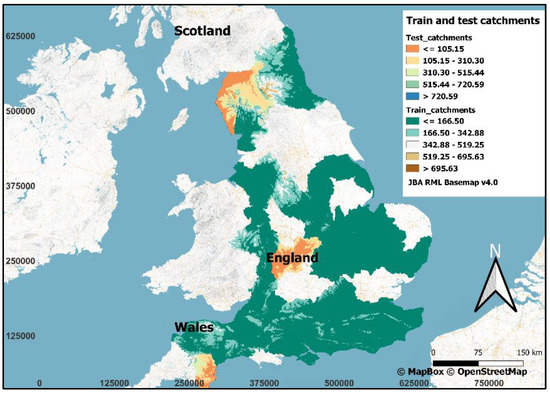
Figure 1.
All training (includes validation catchments) and 3 test catchments.
The target data for the DL model are maximum surface water flood maps generated by a 2D hydraulic model in response to 3 different design storms. We use the proprietary hydraulic model JFlow, developed by JBA Consulting, which solves the 2D shallow water equations and leverages graphics processing units to facilitate large-scale simulations in a swift and efficient manner. A model description and example applications appear elsewhere in the literature [13].
The UK surface water flood map utilizes precipitation depth at a 5 km grid resolution, using the rainfall intensity duration frequency (IDF) model described by [14], (often referred to as the FEH13 model). These IDF curves are translated into event hyetographs for each 5 m × 5 m DEM grid cell used by JFlow using the ReFH2 method that produces a storm profile augmented by losses due to soil storage and urban/rural land classification. The method is described in [15,16].
2.3. U-Net
The U-Net architecture, proposed by Ronneberger and colleagues in 2015 [17], is an autoencoder-like structure equipped with skip connections and is predominantly utilized in image segmentation tasks. The U-Net consists of a contracting pathway designed to encapsulate the context, and a symmetrically expanding pathway that facilitates accurate localization. Skip connections, bridging the contracting and expanding pathways, permit the model to utilize low-level features for high-precision segmentation. U-Net has attained significant popularity within the realm of medical imaging, where it has demonstrated unparalleled performance across a spectrum of segmentation tasks.
2.4. Error Statistics
To assess the performance of the proposed U-Net model in emulating the results of JFlow, the model predictions in terms of maximum water depths are directly compared with the outputs from the hydraulic model. The root-mean-square error (RMSE) [18] and the modified index of agreement (D1) [19] are used to evaluate the overall model performance in capturing the maximum flood depths. In addition, the critical success index (CSI), as used by [11], was used to assess the spatial performance of the predicted maps. The expressions of these indices are described in Table 1.

Table 1.
Evaluation metrics used in this study.
3. Experimental Details
This section provides the key details related to the data pre-processing, the U-Net construction and the model training procedure.
3.1. Data Pre-Processing
In the domain of data-driven modelling, the efficacy of a model is significantly influenced by the quality and relevance of the input data. For flood depth modelling specifically, Löwe et al. [12] identified 11 potential terrain datasets, each encapsulating a wide range of topographical features. However, we could not repeat this given the substantial computational resources and more extensive network architecture that using 11 datasets would necessitate. Our primary focus was on exploring the feasibility of constructing a transferable data-driven model capable of estimating maximum flood depths across various return periods. As such, identifying the optimal set of model inputs was beyond the scope of this investigation and, consequently, we acknowledged that the terrain features used in our model have not been optimized.
The data pre-processing consisted of a four-step process. For the first step, terrain features such as surface elevation, flow accumulation and slope were computed from the DEM. In addition, a drainage mask (binary raster where cells within channels were encoded as ones and the remaining cells were zeros) was used as the fourth input. The resolution of the input data was downgraded from 5 m to 10 m to expedite training times.
The second step involved dividing terrain features by their respective maximum values to rescale the input datasets within a range of 0–1. Additionally, invalid cells were replaced with zero and the target datasets were filtered by assigning a value of zero to depths less than 0.1 m.
For the third step, a systematic patch generation method was used to develop training data patches. This process involved padding the zeros along the catchment boundaries to equalize their sizes, followed by selecting a patch size of 1024 × 1024 using a moving window technique. During this phase, data augmentation techniques, such as vertical and horizontal flipping, were used to increase the size of the training data samples.
For the fourth and final step, the patches from step 3 were stacked to form raster maps composed of multiple image channels. The dimensions of an input patch were set to 2 × 1024 × 1024 × 4, where 2 refers to the batch size (comprising the actual patch and an augmented patch, either vertically or horizontally), 1024 refers to the size of the patch and 4 refers to the number of channels. The dimensions of an output patch were set to 2 × 1024 × 1024 × 3, where the 3 refers to the flood depths corresponding to the 3 design storms (with return periods of 20, 100 and 1000 years).
3.2. U-Net Architecture and Training
We used a U-Net with the aim of maintaining detailed spatial patterns in the outputs while also ensuring a large ‘receptive field’, which refers to the ‘visible pixels’ of the input layer for each output pixel [20]. From a hydrological perspective, a larger receptive field facilitates the capture of water flow from upstream to downstream, which results in water pooling in smaller regions, as the model can learn from global terrain information as opposed to merely local terrain patterns [21]. Consequently, the model’s latent layer (the last layer of the encoder section) possesses a receptive field larger than the input size. We selected an input size of 1024 × 1024 for the U-Net model to retain local and global information, while also ensuring the model’s size was compatible with the computing device and did not exceed memory capacity.
Figure 2 shows the architecture of our U-Net model. Overall, the model comprises four layers, with each layer consisting of two convolutional layers followed by a ‘maxpooling’ layer. We use the ‘Leaky Relu’ activation function in all layers other than the output layer, which uses the ‘rectified linear unit (Relu)’ activation function. The ‘Leaky Relu’ activation function offers two advantages: it circumvents the vanishing gradient problem [22] and mitigates the ‘dead neuron’ issue associated with the ‘Relu’ activation function [23]. The ‘Relu’ function was used in the output layer to ensure that predicted values are always above zero. The ‘kernel size’ of the encoder section was set to 5 × 5, the upsampling (decoder) was 3 × 3 and the ‘maxpooling’ size was 2 × 2.
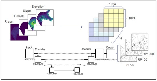
Figure 2.
The U-Net model architecture. Systematically generated patches from the terrain features are stacked as image channels and fed as model inputs; water depths corresponding to 3 return periods are the network outputs. For clarity, not all network layers are shown.
Our U-Net model was constructed using the ‘Keras’ application programming interface (API) in conjunction with Tensorflow 2.5.0. The model’s training was facilitated by the Adam Optimizer [24], which operated with a learning rate of. Due to memory constraints associated with the available graphics card (Nvidia Quadro RTX 5000), a batch size of two was implemented. The model was trained over a span of 2000 epochs, with the mean square error (MSE) serving as the loss function.
Finally, the training process was repeated 3 times using the same network architecture for 3 different training and validation datasets (each time, 20 different catchments were used for training and 5 for validation from a set of 25 catchments). This was done to observe any significant differences in the predicted flood maps when different training and validation data were used. Training the U-Net three times means that we have three models with three different model parameters (weights and biases). These three models can be used independently to predict maximum water depths or can be treated as a three-member ensemble model.
4. Results and Discussion
4.1. Training and Validation Loss
The associated training and validation loss for 2000 epochs is shown in Figure 3. The models continue to exhibit convergence tendencies beyond the 2000 epoch mark, but we ceased training at this point to prevent model overfitting, thereby maintaining their generalizability and performance on unseen data. An additional consideration was the substantial computational time required for the training of a single model (~20 days on average).
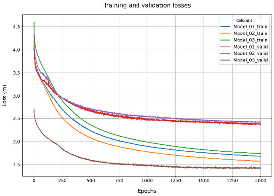
Figure 3.
Training and validation losses for all three U-Net models.
4.2. Assessing the Outputs—Larger Depth for a Larger Event
After the model training, we evaluated the depths corresponding to various return periods. The models need to avoid producing counterintuitive outcomes, such as predicting elevated water levels for storms of lower return periods compared to those with higher return periods. As previously noted, the catchments exhibit overlapping boundaries. Consequently, a comparison of results would not be accurate if a portion of the test catchments were employed for training purposes. To address this issue, we chose three subdomains from each of the catchments for the purpose of comparing depth maps. This approach ensures that the comparisons were based on distinct geographic areas, eliminating the potential bias that could result from overlapping catchment boundaries in the training and test datasets.
Aside from a few minimal discrepancies, we found that the models were indeed capable of predicting increased depths for higher return periods. For instance, following the aggregation process, where maximum depths from all three models were combined into one maximum depth map, one centrally situated test catchment (Area 5404) had a single pixel where the depth associated with a return period of 100 exceeded that of a return period of 1000. Overall, such inconsistencies were noted in 17 pixels spread across the 3 test catchments. Comparatively, the total count of pixels in the case of JFlow maps amounted to 13,790. These observations indicate that the U-Net model’s learning was guided more by global terrain features than local ones, demonstrating its capability for generalization.
4.3. Comparison of U-Net and JFlow Map Outputs
To compare the flood maps, we converted the predicted and the reference (JFlow outputs) water depths into categorical maps. Depth values less than 0.1 m were set to 0 (dry) and otherwise to 1 (wet). The CSI, a commonly used metric for categorical forecasting, was utilized to ascertain the model’s ability to accurately discern wet and dry cells. The CSI encompasses both false alarms and misses, thereby providing a more balanced assessment of actual model performance. The CSI scores indicate that the U-Net model was less accurate than JFlow in detecting wet cells (Table 2). However, a closer look at the flood maps revealed that the U-Net model accurately detected wet cells in regions characterized by channels, tributaries, valleys and sinks, but less accurately in urban environments. This can be attributed to the distinct terrain characteristics of urban areas and the bias in our training data, which predominantly represent rural or semi-urban areas. We also found that the model struggled to accurately simulate flooding along transport lines (roads, railways) and impervious urban areas. At the same time, a clear success was that the model did not predict the presence of water in areas where that would be implausible. Moreover, the model was successful in identifying hotspots, which are areas where water predominantly accumulates.
Table 2.
Error statistics for the test catchments.
4.4. Comparison of U-Net Model and JFlow Depth Outputs
As with the map outputs, we conducted a comparative analysis of the U-Net model’s predicted depths against those from JFlow. For the purposes of comparison of depth, all cells with a water depth less than 0.1 m were assigned a value of 0. This adjustment was implemented consistently across both models. The discrepancies in water depth predictions were systematically quantified using RMSE and D1. The RMSE metric assigns relatively high weights to large errors and was particularly useful when such errors are deemed undesirable. The modified index of agreement, represented by D1, has the advantage of appropriately weighting errors and differences, without inflation due to squared values.
Our analysis revealed a stronger concurrence in the depth maps, though the model consistently underestimated the depths by a smaller margin. Higher D1 values indicate that the U-Net model demonstrates good performance in estimating water depths. However, a worse performance was found for ‘Area 7400’ compared to the other two areas (Table 2). This can be attributed to the unique nature of the terrain in that catchment, where the surface elevation was higher compared to those in the training data.
Figure 4 compares a U-Net-model-predicted flood against an equivalent JFlow-simulated map, also showing the difference between the two. The comparison is consistent with the quantitative error measurements in Table 2, and it is evident that the U-Net model consistently underestimates both the extent and depths of flooding across the test catchments. However, despite the overall discrepancies in the predicted depths, most of the errors tend to cluster within the lowest error band (Figure 4C). While there are instances of large errors, these errors do not occur in areas that should remain void of water accumulation.
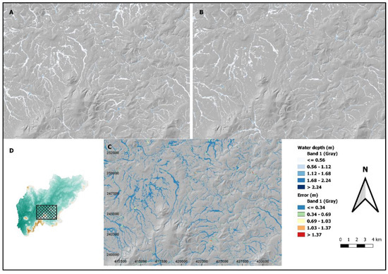
Figure 4.
A visual comparison of water depths between JFlow and U-Net for a 1000-year return period storm event. (A) JFlow-simulated flood map; (B) U-Net-predicted flood map; (C) error map; and (D) map location.
5. Conclusions
We have presented a generalised data-driven model for predicting maximum flood water depths, which demonstrates that advanced DL algorithms can detect flood zones efficiently using terrain attributes.
A key objective of formulating a data-driven model was the rapid production of flood maps. The three U-Net models trained within the scope of this study demonstrate this potential. In this study, we formulated and evaluated three U-Net models for swift flood prediction utilizing topographical features (we aggregated outputs from these models to produce a single flood map for each return period). The findings suggest that the models have the potential to predict flood depths in uncharted catchments across multiple return periods. Nevertheless, the models also frequently underestimate both the depth and extent of water. This underscores the need for further refinement of the model to enhance its accuracy while maintaining its speed, highlighting an avenue for future research and development.
Temporally speaking, each model was capable of estimating depths for three return periods across a domain of approximately 1248 square kilometres within an impressive timeframe of roughly 13 s. Such efficiency may prove valuable in rapid response and planning scenarios, despite the trade-offs inherent in the data-driven approach.
However, our objective was not exclusively to construct a model for either fully urban or rural areas, but rather a hybrid model that encompasses both. The performance of the model could potentially be enhanced through the optimization of network architecture, fine-tuning of hyperparameters and a systematic search for suitable input data. In [12], the authors proposed a forward selection methodology that could potentially be utilized to identify the most suitable set of inputs. Furthermore, it is essential to recognize that strategic selection of terrain features can significantly streamline the process of exploratory data analysis, substantially reducing the time invested in this phase.
Additionally, our observation of significant variability in the water depths predicted by the three models underscores the necessity for a comprehensive assessment of uncertainty. These strategies could collectively contribute to a more robust and accurate model, reinforcing its predictive capacity while also providing a more nuanced understanding of the inherent uncertainty in such predictions.
A trade-off exists between the water depth estimations produced by a hydraulic model and those derived from a data-driven model. Hydraulic models, underpinned by physical laws and centuries’ worth of scientific theory and formulae, are generally deemed more reliable. Conversely, data-driven models do not inherently account for physical constraints, such as mass balance. Given this, one good scenario would be to have a data-driven model capable of generating flood maps expeditiously while maintaining an acceptable margin of error.
Author Contributions
Conceptualization, S.K. and D.W.; methodology, S.K.; software, S.K.; validation, S.K.; formal analysis, S.K.; investigation, S.K.; resources, D.W.; data curation, S.K.; writing—original draft preparation, S.K.; writing—review and editing, S.K., D.W. and S.W.; visualization, S.K.; supervision, D.W.; project administration, S.W. All authors have read and agreed to the published version of the manuscript.
Funding
This research was internally funded by JBA Risk Management.
Institutional Review Board Statement
Not applicable.
Informed Consent Statement
Not applicable.
Data Availability Statement
Training data are proprietary.
Acknowledgments
The DTMs were supplied by Airbus Defence and Space (AD&S), Environment Agency (EA), Natural Resources Wales (NRW) and Bluesky. © Environment Agency copyright and/or database right 2015. All rights reserved. Contains Natural Resources Wales information © Natural Resources Wales and database right. All rights reserved.
Conflicts of Interest
The authors declare no conflict of interest.
References
- Guo, Z.; Leitão, J.P.; Simões, N.E.; Moosavi, V. Data-driven flood emulation: Speeding up urban flood predictions by deep convolutional neural networks. J. Flood Risk Manag. 2021, 14, e12684. [Google Scholar] [CrossRef]
- Guo, Z.; Moosavi, V.; Leitão, J.P. Data-driven rapid flood prediction mapping with catchment generalizability. J. Hydrol. 2022, 609, 127726. [Google Scholar] [CrossRef]
- Kabir, S.; Patidar, S.; Xia, X.; Liang, Q.; Neal, J.; Pender, G. A deep convolutional neural network model for rapid prediction of fluvial flood inundation. J. Hydrol. 2020, 590, 125481. [Google Scholar] [CrossRef]
- Kochkov, D.; Smith, J.A.; Alieva, A.; Wang, Q.; Brenner, M.P.; Hoyer, S. Machine learning–accelerated computational fluid dynamics. Proc. Natl. Acad. Sci. USA 2021, 118, e2101784118. [Google Scholar] [CrossRef] [PubMed]
- Bates, P.D.; De Roo, A.P.J. A simple raster-based model for flood inundation simulation. J. Hydrol. 2000, 236, 54–77. [Google Scholar] [CrossRef]
- Neal, J.; Dunne, T.; Sampson, C.; Smith, A.; Bates, P. Optimisation of the two-dimensional hydraulic model LISFOOD-FP for CPU architecture. Environ. Model. Softw. 2018, 107, 148–157. [Google Scholar] [CrossRef]
- Crossley, A.; Lamb, R.; Waller, S. Fast solution of the shallow water equations using GPU technology. In Proceedings of the BHS Third International Conference—Managing Consequences of a Changing Global Environment, Newcastle upon Tyne, UK, 19–23 July 2010. [Google Scholar]
- Xia, X.; Liang, Q.; Ming, X. A full-scale fluvial flood modelling framework based on a high-performance integrated hydrodynamic modelling system (HiPIMS). Adv. Water Resour. 2019, 132, 103392. [Google Scholar] [CrossRef]
- Guidolin, M.; Chen, A.S.; Ghimire, B.; Keedwell, E.C.; Djordjević, S.; Savić, D.A. A weighted cellular automata 2D inundation model for rapid flood analysis. Environ. Model. Softw. 2016, 84, 378–394. [Google Scholar] [CrossRef]
- Donnelly, J.; Abolfathi, S.; Pearson, J.; Chatrabgoun, O.; Daneshkhah, A. Gaussian process emulation of spatio-temporal outputs of a 2D inland flood model. Water Res. 2022, 225, 119100. [Google Scholar] [CrossRef] [PubMed]
- do Lago, C.A.F.; Giacomoni, M.H.; Bentivoglio, R.; Taormina, R.; Gomes, M.N.; Mendiondo, E.M. Generalizing rapid flood predictions to unseen urban catchments with conditional generative adversarial networks. J. Hydrol. 2023, 618, 129276. [Google Scholar] [CrossRef]
- Löwe, R.; Böhm, J.; Jensen, D.G.; Leandro, J.; Rasmussen, S.H. U-FLOOD—Topographic deep learning for predicting urban pluvial flood water depth. J. Hydrol. 2021, 603, 126898. [Google Scholar] [CrossRef]
- Lamb, R.; Crossley, M.; Waller, S. A fast two-dimensional floodplain inundation model. Water Manag. 2009, 162, 363–370. [Google Scholar] [CrossRef]
- Stewart, E.J.; Jones, D.A.; Svensson, C.; Morris, D.G.; Dempsey, P.; Dent, J.E.; Collier, C.G.; Anderson, C.A. Reservoir Safety—Long Return Period Rainfall. Available online: https://assets.publishing.service.gov.uk/media/602e43e2e90e0709e3127489/_long_return_report_1.pdf (accessed on 21 July 2023).
- Kjeldsen, T.R. The revitalised FSR/FEH rainfall-runoff method. In FEH Supplementary Report No. 1; Centre for Ecology & Hydrology: Wallingford, UK, 2007. [Google Scholar]
- Kjeldsen, T.R.; Miller, J.D.; Packman, J.C. Modelling design flood hydrographs in catchments with mixed urban and rural land cover. Hydrol. Res. 2013, 44, 1040–1057. [Google Scholar] [CrossRef]
- Ronneberger, O.; Fischer, P.; Brox, T. U-Net: Convolutional Networks for Biomedical Image Segmentation. In Medical Image Computing and Computer-Assisted Intervention—MICCAI 2015; Navab, N., Hornegger, J., Wells, W.M., Frangi, A.F., Eds.; Springer International Publishing: Cham, Switzerland, 2015; pp. 234–241. [Google Scholar]
- Barnston, A.G. Correspondence among the Correlation, RMSE, and Heidke Forecast Verification Measures; Refinement of the Heidke Score. Weather. Forecast. 1992, 7, 699–709. [Google Scholar] [CrossRef]
- Willmott, C.J. On the Evaluation of Model Performance in Physical Geography. In Spatial Statistics and Models; Gaile, G.L., Willmott, C.J., Eds.; Springer: Dordrecht, The Netherlands, 1984; pp. 443–460. [Google Scholar] [CrossRef]
- Luo, W.; Li, Y.; Urtasun, R.; Zemel, R. Understanding the Effective Receptive Field in Deep Convolutional Neural Networks. arXiv 2017, arXiv:1701.04128. [Google Scholar]
- Geirhos, R.; Rubisch, P.; Michaelis, C.; Bethge, M.; Wichmann, F.A.; Brendel, W. ImageNet-Trained CNNs Are Biased towards Texture; Increasing Shape Bias Improves Accuracy and Robustness. 2018. Available online: http://arxiv.org/abs/1811.12231 (accessed on 16 May 2023).
- Hochreiter, S. The Vanishing Gradient Problem During Learning Recurrent Neural Nets and Problem Solutions. Int. J. Uncertain. Fuzziness Knowl.-Based Syst. 1998, 6, 107–116. [Google Scholar] [CrossRef]
- Nair, V.; Hinton, G.E. Rectified Linear Units Improve Restricted Boltzmann Machines. In Proceedings of the 27th International Conference on International Conference on Machine Learning, Madison, WI, USA, 21–24 June 2010; pp. 807–814. [Google Scholar]
- Kingma, D.P.; Ba, J. Adam: A Method for Stochastic Optimization. arXiv 2014, arXiv:1412.6980. [Google Scholar]


Disclaimer/Publisher’s Note: The statements, opinions and data contained in all publications are solely those of the individual author(s) and contributor(s) and not of MDPI and/or the editor(s). MDPI and/or the editor(s) disclaim responsibility for any injury to people or property resulting from any ideas, methods, instructions or products referred to in the content. |
© 2023 by the authors. Licensee MDPI, Basel, Switzerland. This article is an open access article distributed under the terms and conditions of the Creative Commons Attribution (CC BY) license (https://creativecommons.org/licenses/by/4.0/).