Reduced Order Modeling with Skew-Radial Basis Functions for Time Series Prediction ^†

Abstract

We present a sparsity-promoting RBF algorithm for time-series prediction. We use a time-delayed embedding framework and model the function from the embedding space to predict the next point in the time series. We explore the standard benchmark data set generated by the Mackey–Glass chaotic dynamical system. We also consider a model of temperature telemetry associated with the mouse model immune response to infection. We see that significantly reduced models can be obtained by solving the penalized RBF fitting problem.

1. Introduction

Radial basis functions (RBFs) provide an attractive option for the fitting of data in high-dimensional domains. They are appealing for their simplicity and compact nature while enjoying universal approximation theorems suggesting, in principle, that they are potentially as powerful as other methodologies. Traditional RBF expansions are of the form

$$f\left(x\right)=\sum _i{w}_i\varphi (\parallel x-c_i\parallel )$$

(1)

where $f:\mathbb{R}\to \mathbb{R}$, and the function $\varphi (·)$ is selected from a variety of options including functions such as $\{r,r^3,r^{2}lnr,exp(-r),exp(-r^2),\dots \}$ and placed at points $\left\{c_i\right\}$. Unlike the fully nonlinear optimization problems encountered with multilayer perceptrons, recurrent neural networks, and deep convolutional networks, the weights in RBF expansions can be determined by solving aleast-squares problem. The RBF centers $\left\{c_i\right\}$ can be found using a variety of approaches including random selection, clustering, or nonlinear optimization. The added property of skewness, introduced in [1], makes an RBF-based approach more powerful at fitting asymmetric features in the data.

Skew-radial basis functions (sRBF) introduce the symmetry-breaking function $s_i:\mathbb{R}\to \mathbb{R}$ for each center, i.e.,

$$f\left(x\right)=\sum _i{w}_i{s}_i(x;D_i)\varphi (\parallel x-c_i{\parallel }_{W_i})$$

(2)

The matrix $D_i$ consists of the skew shape parameters, and $W_i$ is a diagonal weighting for the Euclidean inner product.

Radial basis functions were introduced as an alternative to artificial neural networks for function approximation based on the flexibility of the optimization problem [2]. They have proven particularly useful for both reduced-order and adaptive, or online modeling of data-streams. Given that the contribution of each individual basis function to the complexity of the model is easily interpreted, they may be sequentially placed where they are most needed until the data are fitted [3]. Alternatively, one can employ linear programming to adapt a model as changes are detected in the distributions of the data [4]. A comprehensive review of the RBF literature may be found in [5].

2. Sparse Skew RBFs

Building off of traditional RBF (1) and skew RBF formulation (2), we introduce sparsity via $L_1$ penalization for the number of centers via the solution of the optimization problem

$$\underset{\{w_i,W_i,D_i,c_i\}}{min}∥y-\sum _{i=1}^{n_c}{w}_i{s}_i(x;D_i)\varphi \left(d_i(x,c_i;W_i)\right)∥+\alpha \sum _{i=1}^{n_c}\left|w_i\right|$$

(3)

We follow the choices in [1] (Section 4.3) for choice of $s_i$ and $\varphi$. The per-center inner product and induced norm for a single center $c_i$ with u, $v\in {\mathbb{R}}^n$ are

$${⟨u,v⟩}_{W_i}=u^T{W}_i{v;\left|\right|u\left|\right|}_{W_i}=\sqrt{{⟨u,u⟩}_{W_i}}$$

(4)

with a symmetric positive definite $W_i$. The metric is $d_i(x,c_i;W_i)={\parallel x-c_i\parallel }_{W_i}$, and choice of base RBF $\varphi \left(r\right)=exp(-r^2)$ unless stated otherwise. The skew functions $s_i$ have shape parameters that are optimized for each basis function. We specialize to skew matrices which are diagonal; $D_i=\mathrm{diag}\left({\lambda }_i\right)$, ${\lambda }_i\in {\mathbb{R}}^n$; so

$$s_i(x;{\lambda }_i)=\frac{1}{\pi }arctan\left({\lambda }_i^T(x-c_i)\right)+\frac{1}{2}$$

(5)

so $s_i:{\mathbb{R}}^n\to (0,1)$. Using diagonal $D_i$ parameter matrix produces a skew which is interpreted as having a direction and magnitude of effect; see Figure 1 for an illustration of this idea with a single sRBF in ${\mathbb{R}}^2$.

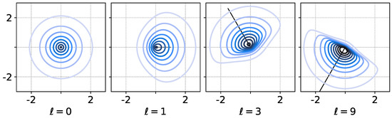
Figure 1. Visualization of level sets a single skew RBF as in Equation (2) in ${\mathbb{R}}^2$ using $W=I$ and diagonal $D=\mathrm{diag}(\ell cos(\theta ),\ell sin(\theta \left)\right)$. Setting $\ell =0$ ($D=0$) restores symmetry. Various $\theta$ and ℓ (vectors shown in panels) directly correspond to a direction and magnitude of asymmetry in the RBF. Further shape control comes with choice of Euclidean W-norm (not shown).

We have solved the optimization problem in Equation (3) to compute a parsimonious expansion given by Equation (2). For scalar time series, this is performed using a time-delay embedding of the series $\{x_1,x_2,x_3,\dots \}$, where the fitting problem becomes a map from an l-dimensional embedding space to the next time-point of interest, e.g.,

$$x_{n+1}=f(x_n,x_{n-T},x_{n-2T})$$

(6)

where typically we choose $l=3$, and T is a delay time for sampling the time series at uncorrelated points. In this approach we are solving this optimization problem in batch mode, i.e., we assume that the complete data set is available for training. This is in contrast to [6], where RBFs are sequentially placed based on a statistical test, or in [4], where the RBFs are placed incrementally for streaming data. Note that [4] also employs the one-norm in the optimization problem, but it is solved using the dual simplex algorithm rather than gradient-based methods we use here. The optimization problem in Equation (3) is readily solved in Python, via PyTorch, which provides automatic differentiation and optimization tools.

3. Numerical Results

3.1. Details of Implementation

Each scalar time series is mean-centered using values from the training data prior to time-delay embedding.

We use PyTorch as a framework to implement the mixed-objective loss (3). PyTorch provides a large collection of tools for a user to define arbitrary loss functions and optimization techniques. We subclassed torch.nn.Module, allowing us to pass a collection of parameters and save the history during the learning phase. Updates were found using torch.optim.SGD with learning rate 0.1 and sometimes enabling Nesterov momentum, though we expect the details of these choices have no noticeable impact on our downstream conclusions.

The entirety of input/output training data $(X,y)$ with $X\in {\mathbb{R}}^{n\times N}$, $y\in {\mathbb{R}}^N$ (N samples) are given to the module in the training phase (in contrast to online learning). For larger time series, we trained using simple uniform random batches of 5% of the training data on each iteration. Unless stated otherwise, the objective is the one-step prediction for $y_n:=x_{n+1}$ based on input $X_n:=(x_n,x_{n-T},x_{n-2T})$.

3.2. Mackey–Glass Revisited

We begin our exploration of the sparse skew RBFs by solving the optimization problem given by Equation (3) for various parameter configurations. For this first numerical experiment, we use the Mackey–Glass chaotic time series, a standard for benchmarking RBF algorithms [3]. We employ 1197 points time-delayed and embedded into three dimensions to predict the next point. We used 800 points for training, 200 points for validation, and reserved an additional 195 for testing. In all our experiments, the prediction accuracies on training, validation, and test data were very similar, indicating no overfitting was taking place. Note that our current goal is to explore the behavior of the proposed algorithm for different parameters, rather than perform a head-to-head comparison with other algorithms. This frees us to select the modeling set-up from scratch and not be bound to choices made in other papers. Here we take $T=1$.

It is useful to explore the sparsity behavior of the model as a function of the parameter $\alpha$; we select the values shown in Table 1. All the results in this paper used 50,000 epochs for training. In Table 1, we see that, as expected, the number of skew RBFs with weight $|W_i|$ > $1e-3$ decreases with increasing $\alpha$. Interestingly, for $\alpha =0.002$, we see a sharp drop in the absolute value of the weights. The resulting model requires only two RBFs and has relatively low error. Note that we also saw similar behavior with model size $n_c$ = 20,100.

Table 1. This table shows the variability of the model order (number of numerically nonzero sRBF weights) as a function of the sparsity parameter $\alpha$.

Number of Centers = 50
Sparsity$\mathbf{\alpha }$	${\parallel \mathit{w}\parallel }_{\mathbf{1}}$	Train Acc	Val Acc	RBFs
0	26.84	0.0013	0.0012	50
0.0001	19.47	0.0009	0.0007	50
0.002	2.14	0.0024	0.0021	2
0.01	1.66	0.0036	0.0033	1
0.1	1.28	0.0177	0.0169	1

In Figure 2, we plot the absolute values of the skew RBF expansion weights $w_i$ sorted in decreasing order. We see how the distribution of weights is impacted by the sparsity parameter with $\alpha =0.002$ versus $\alpha =0$. Here, with the sparsity parameter $\alpha =0.002$, the model selects two optimal RBFs that produce an error of $0.0021$ versus the 50 skew RBF model (with $\alpha =0$) that results in an error of $0.0012$. Interestingly, the 1-norm penalized model with $\alpha =0.0001$ still uses 50 skew RBFs but has the smallest error of all the models. In Figure 3 (top), we plot the model prediction that uses 50 RBFs and $\alpha =0$. In contrast, in Figure 3 (bottom) we see the results of an RBF with two basis functions approximating the Mackey–Glass time series. The smaller model fails to capture the positive extreme values, but only 2 skew RBFs are used in contrast to 50 skew RBFs.

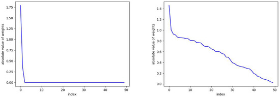
Figure 2. The parameter $\alpha$ can be seen here to promote sparsity. On the left, $\alpha =0.002$ and the number of required skew RBFs is 2. On the right, we take $\alpha =0$ and there is no sparsity and 50 skew RBFs are used in the model. See Figure 3 for the corresponding predictions.

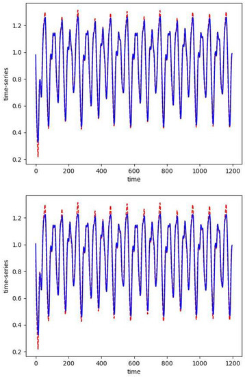
Figure 3. The one-step prediction (blue) of the Mackey–Glass time series (red). The first 800 points are training data. For both simulations we take $n_c=50.$ Top: as expected, with $\alpha =0$, the solution of the optimization problem requires 50 skew basis functions. Bottom: with $\alpha =0.002$ the sparse solution only uses 2 skew RBFs.

We remark that this approach differs from the benchmarking in [6], where noise was added to the data and the mapping used a four-dimensional domain. The approach used in [6] requires the presence of noise since the approach employs a noise test on the residuals. Here we are using an optimization that uses all the available data. This is in contrast to methods that build the model in a streaming fashion, i.e., online, adding one point at a time as they become available [4,6].

3.3. Mouse Telemetry Data

The collection of data here are the result of experiments on laboratory mice conducted by the Andrews-Polymenis and Threadgill labs [7,8,9]. The broad question is to identify mechanisms of tolerance and understand the variety of immune response to a few specific diseases in mice. The time series are the result of surgically embedding a device which tracks internal body temperature (degrees Celsius) and activity (physical movements) sampled at 1/60 Hz (once per minute). Mice are left alone for approximately 7 days, then infected, and then further observed for an additional 7–14 days before being euthanized. We focus on the temperature time series here.

The process of numerically finding a zero-autocorrelation time to find a delay for TDE leads us to a delay $T=4\sim 6$ h. Alternatively, a theoretical argument for studying autocorrelation of the monochromatic signal $sin(2\pi t/\tau )$ leads to guidance of choosing $T=\tau /4$, i.e., one-fourth of the period. Assuming mice exhibit circadian behavior (a period of 24 h), this agrees with numerical studies and so we use $T=24/4=6$ h. The training process and results of this process are visualized in Figure 4.

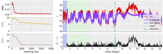
Figure 4. (Left): Decay of loss during training and diagram of associated time series. The mean-square error quickly saturates while one-norm of weight vector w slowly decays. Only a handful of non-zero model centers ${\left|\right|w\left|\right|}_0$ persist past the first 1000 iterations. (Right): Approximate mean-normalization is applied, followed by a delay (blue region) for TDE. The model is trained on three days of data (green region). The original time series (red, dashed) and model prediction of the learned model (solid purple) are shown. Pointwise prediction error of $x\left(t\right)$ is shown beneath. Parameters: $\alpha =0.01$, $n_c=21$, $T=360$, $l=3$.

3.4. Other Applications

3.4.1. Iterated Prediction

We study how our sRBF implementation can be directly interpreted and how it can be applied to anomaly detection. One method of evaluating the success of the trained model is to study iterated prediction rather than repeated one-step prediction. Given an initial training set, the task is to repeatedly feed the output of the model as new input; e.g.,

$$\begin{array}{cc}\hfill & f(x_t,x_{t-T},x_{t-2T})\to {\widehat{x}}_{t+1}\hfill \end{array}$$

(7)

$$\begin{array}{cc}\hfill & \Rightarrow f({\widehat{x}}_{t+1},x_{t-T+1},x_{t-2T+1})\to {\widehat{x}}_{t+2}\hfill \end{array}$$

(8)

$$\begin{array}{cc}\hfill & \Rightarrow \dots \hfill \end{array}$$

(9)

The broad question is to ask, “Did the model in fact learn the shape of my data?” The answer may be yes quantitatively if the time series continues to have small prediction error without further training or online learning applied. More holistically, we are interested in whether the time series learns a (quasi)periodic shape by approaching a limit cycle. Figure 5 illustrates this idea with a noiseless sine wave. One-step prediction (red) is successful; iterated prediction (purple) receives no further ground-truth, with some evidence towards the existence of a limit cycle. Similar application with a mouse time series in Figure 5 (bottom) succeeds in one-step prediction, but the iterated prediction exhibits behavior akin to an exponential decay to a fixed point.

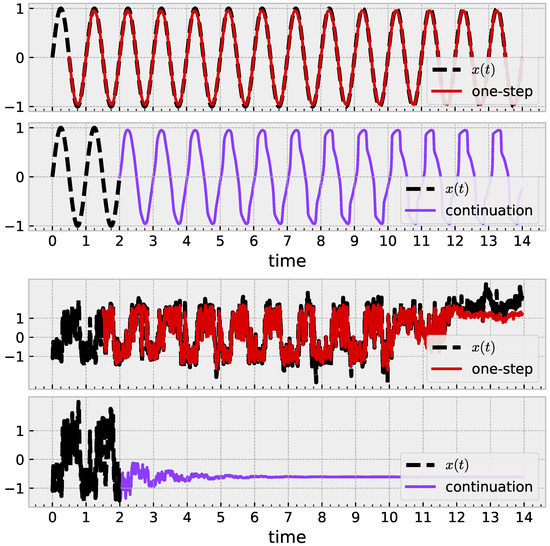
Figure 5. Results illustrating how a trained sRBF model learns geometric structure. (Top): With $sin\left(t\right)$, a learned model leads to a limit cycle. (Bottom): Similar approach with noisy mouse data fails. Parameters $\alpha =0.01$, $n_c=21$, $l=3$. After training, both models decrease to 3 active centers.

3.4.2. Visualization of Trained sRBF Models

When the embedding dimension of a scalar time series is $l=2$, we can reason about and explain the model with the full set of learned parameters in Equation (2). Figure 6 illustrates this idea with one such mouse time-series model. Following the expectation for $L_1$ penalization in the training objective, we consider weights $|w_i |<1e-2$ to be numerically zero and then build the full function $f:{\mathbb{R}}^2\to \mathbb{R}$ in analogy to the single sRBF illustrations in Figure 1. We emphasize careful interpretation with this figure. Red crosses represent locations of sRBF centers, which may not directly align with local extrema due to the asymmetry. Next, contour colors represents the value associated with the the prediction for $x_{t+1}$, which cannot be directly visualized in the plane here. Ideally, we would like to understand how the learned model positions centers and shapes parameters to match the embedded time series in ${\mathbb{R}}^2$ but requires subsequent visualization of time-series values. We leave this for future work.

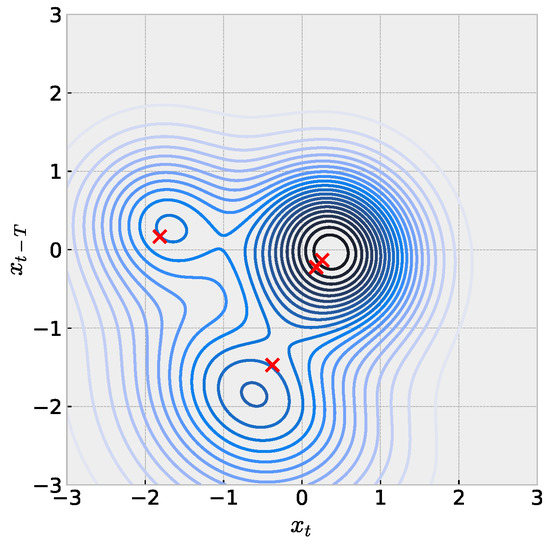
Figure 6. Visualization of sRBF model trained with mouse time series embedded in dimension $l=2$. Red crosses mark sRBF centers, which may not be located with local maxima due to asymmetry. Parameters: $\alpha =0.01$, $n_c=21$, $l=2$.

3.4.3. Anomaly Detection

An important application area for time series modeling, especially with health data such as these, is anomaly detection. An anomaly can signal need for treatment, adjustment, intervention, etc. Additionally, it is important to carefully consider how to train such a model and how to evaluate success (or failure) depending on the specific application. Figure 7 illustrates these ideas with one such temperature time series. Here, the shaded green region marks training data, which is assumed “nominal” or “healthy” data (and in general requires knowledge of the application area). Square marks in darker shades of green on the time series denote detected anomalies. The definition of an anomaly can depend on the specific modeling approach; but often involves producing a scoring system (some function which maps input data to $[0,\infty )$ or $[0,1]$) which can be thresholded to produce a binary decision of “nominal” or “anomaly”. Ultimately, the threshold is a free parameter, and one mediates between false positives and negatives based on the choice. This figure illustrates two automated methods for choosing a threshold based on quantiles. The more sensitive of the two shown is a decision based on a new pointwise prediction error $|{\widehat{x}}_{t+1}-x_{t+1}|$ being greater than 99% of such errors in the training data. Increasing this threshold reduces sensitivity but hopefully also reduces false positives (the meaning of which is also dependent on the application). Anomaly detection remains challenging without applying a full time-series analysis pipeline which denoises or directly models noise, and we leave a more thorough investigation of the application of skew RBFs to this task to future work.

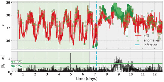
Figure 7. Anomaly detection based on thresholding error in one-step prediction $|\widehat{y}-x_{t+1}|$ exceeding a threshold of error built from training data.

4. Conclusions

In summary, we have proposed an approach for computing reduced order skew RBF approximations. This approach is complementary to others in the literature that seek to construct a parsimonious fit with RBFs. This batch method approach is appealing for its algorithmic simplicity. The fact that the number of required RBFs can be determined by the steep drop in expansion weights makes it appealing for automatic model order determination. In the future, it would be interesting to explore the annealing of the sparsity coefficient during training.

We note that there has been a renewed interest in RBFs in view of the observation that kernel methods, under certain circumstances, can be viewed as equivalent to deep neural networks [10]. The use of a weighted Euclidean inner product may be viewed as a featurization of the data, while the kernel expansion completes the data fitting. Thus, this renewed attention to the optimization problems associated with radial basis functions may be of broad interest.

References

- Jamshidi, A.; Kirby, M. Skew-Radial Basis Function Expansions for Empirical Modeling. SIAM J. Sci. Comput. 2010, 31, 4715–4743. [Google Scholar] [CrossRef]
- Broomhead, D.; Lowe, D. Multivariable Functional Interpolation and Adaptive Networks. Complex Syst. 1988, 2, 321–355. [Google Scholar]
- Jamshidi, A.A.; Kirby, M.J. A Radial Basis Function Algorithm with Automatic Model Order Determination. SIAM J. Sci. Comput. 2015, 37, A1319–A1341. [Google Scholar] [CrossRef]
- Ma, X.; Aminian, M.; Kirby, M. Incremental Error-Adaptive Modeling of Time-Series Data Using Radial Basis Functions. J. Comput. Appl. Math. 2019, 362, 295–308. [Google Scholar] [CrossRef]
- Jamshidi, A. Modeling Spatio-Temporal Systems with Skew Radial Basis Functions: Theory, Algorithms and Applications. Ph.D. Dissertation, Colorado State University, Department of Mathematics, Fort Collins, CO, USA, 2008. [Google Scholar]
- Jamshidi, A.; Kirby, M. Modeling Multivariate Time Series on Manifolds with Skew Radial Basis Functions. Neural Comput. 2011, 23, 97–123. [Google Scholar] [CrossRef] [PubMed]
- Aminian, M.; Andrews-Polymenis, H.; Gupta, J.; Kirby, M.; Kvinge, H.; Ma, X.; Rosse, P.; Scoggin, K.; Threadgill, D. Mathematical methods for visualization and anomaly detection in telemetry datasets. Interface Focus 2020, 10, 20190086. [Google Scholar] [CrossRef]
- Scoggin, K.; Gupta, J.; Lynch, R.; Nagarajan, A.; Aminian, M.; Peterson, A.; Adams, L.G.; Kirby, M.; Threadgill, D.W.; Andrews-Polymenis, H.L. Elucidating mechanisms of tolerance to Salmonella typhimurium across long-term infections using the collaborative cross. MBio 2022, 13, e01120-22. [Google Scholar] [CrossRef] [PubMed]
- Scoggin, K.; Lynch, R.; Gupta, J.; Nagarajan, A.; Sheffield, M.; Elsaadi, A.; Bowden, C.; Aminian, M.; Peterson, A.; Adams, L.G.; et al. Genetic background influences survival of infections with Salmonella enterica serovar Typhimurium in the Collaborative Cross. PLoS Genet. 2022, 18, e1010075. [Google Scholar] [CrossRef]
- Radhakrishnan, A.; Beaglehole, D.; Pandit, P.; Belkin, M. Feature learning in neural networks and kernel machines that recursively learn features. arXiv 2022, arXiv:2212.13881. [Google Scholar]
Disclaimer/Publisher’s Note: The statements, opinions and data contained in all publications are solely those of the individual author(s) and contributor(s) and not of MDPI and/or the editor(s). MDPI and/or the editor(s) disclaim responsibility for any injury to people or property resulting from any ideas, methods, instructions or products referred to in the content. |
© 2023 by the authors. Licensee MDPI, Basel, Switzerland. This article is an open access article distributed under the terms and conditions of the Creative Commons Attribution (CC BY) license (https://creativecommons.org/licenses/by/4.0/).