Tropospheric and Ionospheric Modeling Using GNSS Time Series in Volcanic Eruptions (La Palma, 2021) ^†

Abstract

The signal coming from the artificial satellites of the GNSS system suffers various effects that considerably decrease the precision in solving the positioning problem. To mathematically model these effects, the atmosphere is divided into two main parts, the troposphere and the ionosphere. The troposphere can only be modelled, while the ionospheric effect can be modeled or eliminated depending on the geodetic sophistication of the receivers used. In this way, information is obtained about both layers of the atmosphere. For tropospheric modeling, the parameters of total zenithal delay (ZTD) or precipitable water vapor (PVW) will be taken, and for the ionosphere the total electron content (TEC) will be taken. In this work, statistical and analytical techniques will be applied with the R software; for example, ARMA, ARIMA models, least squares methods, wavelet functions, Kalman techniques, and CATS analysis. With this, the anomalies that occurred in the values of the ZTD and TEC in the case of the 2021 eruption of the Cumbre Vieja volcano on the island of La Palma.

1. Introduction

The GNSS systems composed by GPS (USA), Glonass (Russia), Galileo (European Union), and Beidou (China), in addition to solving the problem of precise positioning, provide information on the delay in the propagation of the signal as it passes through the troposphere and the ionosphere.

Most meteorological events occur in the troposphere, so the variability of the tropospheric delay depends directly on the meteorological conditions at the time of study, considering the temperature, humidity and atmospheric pressure, the PWV (Precipitable Water Vapor) value is obtained from the ZTD value. This dependence between the two parameters means that the study of tropospheric delay is related to the calculation of precipitable water vapor.

The ionosphere is characterized by its total electron content (TEC), which will affect the propagation of the GNSS-GPS signal. Ionization is caused, mainly, by ultraviolet radiation from the Sun; and with this there are maximum values of TEC during the day and minimum values at night. Solar activity is characterized through the number of sunspots produced by the Sun, solar cycles have been detected every 11 years and supercycles between 80 and 100 years; however, some works relate ionospheric disturbances with seismic and volcanic phenomena [1].

Tropospheric delay can be modeled using different tropospheric models. For the study of the ionospheric delay, the combination of the frequencies $L_1$ and $L_2$ has been used. Thus, obtaining the frequency $L_4$ and, by its definition, the value of the TEC. In this work, the data modeling has been carried out using the Bernese 5.2 software [2].

This work will focus on the study of the ZTD and TEC values in the island of La Palma and surroundings during the pre-eruption, eruption, and post-eruption of Cumbre Vieja volcano using different statistical and analytical techniques, such as ARMA, ARIMA, and Kalman, and STL decomposition using R 4.1.2 software.

2. Experimental Background

2.1. Geodynamic Background

La Palma is part of the volcanic archipelago of the Canary Islands that is one of the southern archipelagos of the African Atlantic border, together with Madeira, the Savage Islands, and Cape Verde [3].

The Canary Islands archipelago is located in the interior of the African Plate, presenting volcanic and tectonic activity. All these islands have been formed from volcanic eruptions; it could be said that it is a volcanically active area.

The following table shows the latest eruptions in the Canary archipelago [4]:

Year	Island	Denomination
1712	La Palma	Eruption of El Charco (Montaña Lajiones)
1730–1736	Lanzarote	Eruption of Timanfaya
1798	Tenerife	Volcano Pico Viejo (Narices del Teide)
1824	Lanzarote	Volcano de Tao, Volcano Nuevo del Fuego y Volcano nuevo
1909	Tenerife	Volcano Chinyero
1949	La Palma	Volcano Hoyo Negro, Durazanero, Llano del Banco
1971	La Palma	Volcano Teneguía
2011–2012	El Hierro	Volcano del mar de las Calmas
2021	La Palma	Volcano Cumbre Vieja

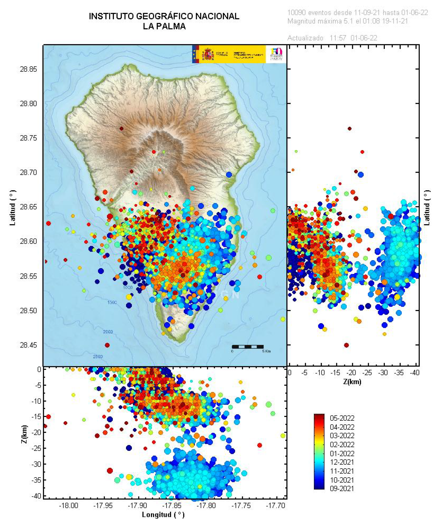
Before the eruption of the Cumbre Vieja volcano, the island of La Palma was considered an area with low seismicity; however, in 2017, seismic swarms of low intensity and at great depth began to occur. It was not until June 2021 when more and more seismic events began to be experienced on the island of La Palma, but a week before the eruption is when there were a large number of seismic swarms whose depth was decreasing, this being a powerful indication of the imminent eruption (See Figure 1).

2.2. Description of Selected Series

To carry out the study on how the eruption of the La Palma volcano has been influenced, the time series provided by the Bernese Software 5.2, corresponding to the values of ZTD and TEC, will be taken, which refer to the delay produced in the propagation of the signal from satellites to permanent GNSS stations as it passes through the atmosphere. In addition, the data will be expanded, in the case of ZTD values, making use of the GNSS stations provided by the Nevada Geodetic Laboratory (NGL).

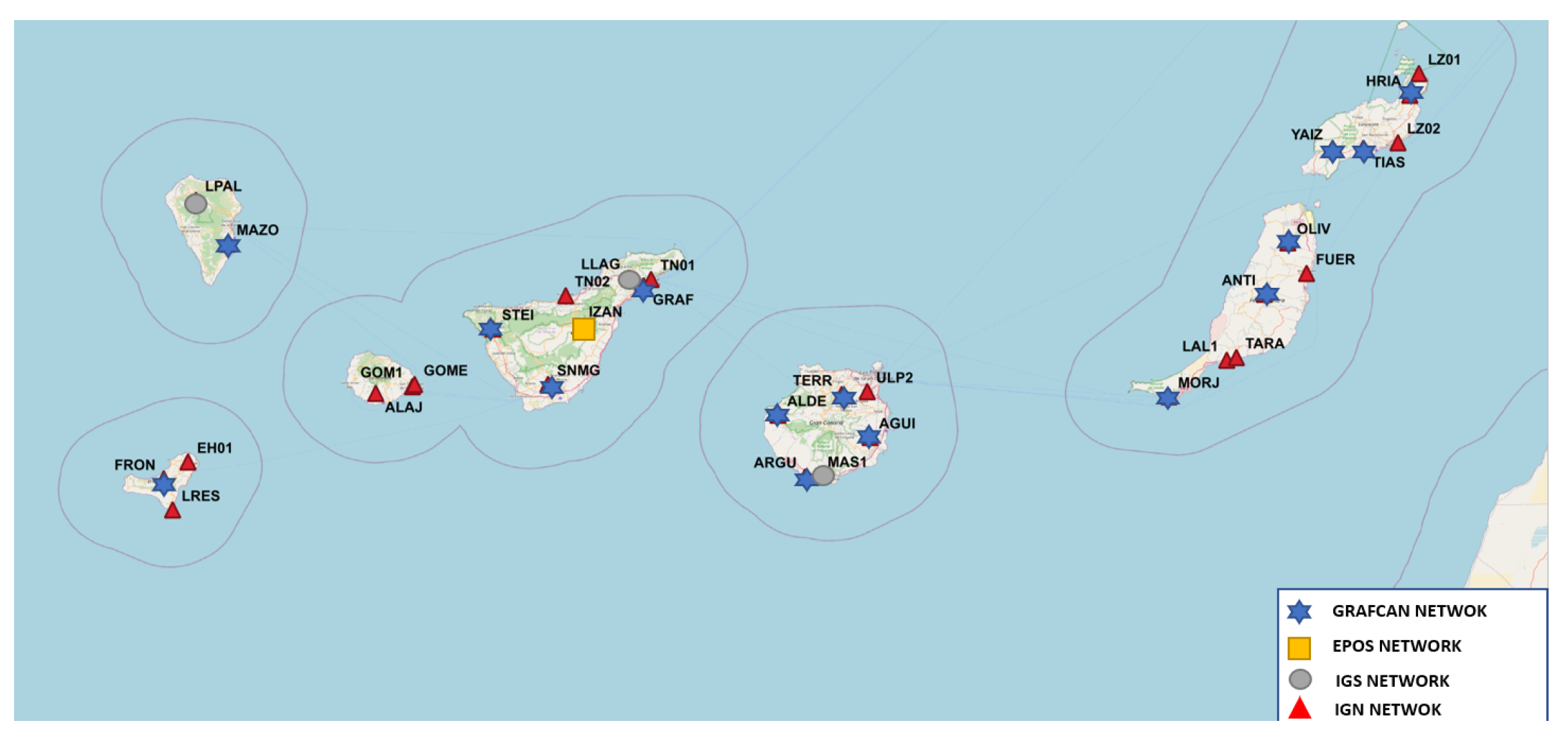
For this purpose, GPS stations located on the different islands that make up the Canary archipelago and that belong to the MAGNET network provided by NGL will be taken [5] (See Figure 2):

• La Palma: Garafia (LPAL), Villa de Mazo (MAZO).
• La Gomera: San Sebastián de La Gomera (GOME, GOM1), Alarejó (ALAJ).
• El Hierro: La Restinga (LRES), Frontera (FRON), Valverde (EH01).
• Tenerife: Güímar (IZAN), Santiago del Teide (STEI), San Miguel de Abona (SNMG), Santa Cruz de Tenerife (GRAF), La Laguna (LLAG), Santa cruz de Tenerife (TN01), Puerto de la Cruz (TN02).
• Gran Canarias: La Aldea de San Nicolás (ALDE), Teror (TERR), Agüimes (AGUI), Aguineguín (ARGU), Tafira Baja (ULP2), Maspalomas (MAS1).
• Lanzarote: Haría (HRIA), Yaiza (YAIZ), Tías (TIAS), Órzola (LZ01), Arrecife (LZ02).
• Fuerteventura: Morro Jable (MORJ), Tarajalejo (TARA), Antigua (ANTI), La Oliva (OLIV), Puerto del Rosario (FUER), La Lajita (LAL1).

3. Analytical and Statistical Techniques

GPS satellites have been used in this work. The GPS time series formed by the data from the ZTD and TEC values are a priori corrected when processing the data sent by the satellites to the GPS permanent stations. These values provide information on the atmospheric delay produced in the path of the GPS signal traveling from the satellites to a given GPS station.

These data usually contain outliers, so initial filtering must be used on the series obtained to eliminate them. Once the filtered series is obtained, analytical and statistical techniques can be applied to proceed to a descriptive analysis of the series.

For this study, ZTD and TEC values obtained through the Bernese 5.2 software will be taken. In addition, the number of permanent GNSS-GPS stations from which ZTD values are obtained will be increased, using the data provided by the NGL laboratory [6].

3.1. Initial Filters of the Series

The objective of any initial filtering that is applied to the GPS series consists of the elimination of data with very different values, outliers, from the rest of the series. In the case of non-linear series, this process is carried out by linear sections within the series. On the other hand, R contains a package, forecast, to filter time series data, that is based on the Box–Cox transform [7,8] and is completed by the tsoutliers() function. It is used to achieve greater linearity, homoscedasticity and a tendency towards a normal distribution of the values of the series.

3.2. Kalman

For this filtering, it is necessary to know what the dynamic linear models are like; assuming they are known, we proceed to define the Kalman filtering [9]. The Kalman filter is of a predictive–corrective type, as the parameter ${\theta }_t$ that determines the state of the model at time t is calculated, the estimation of the observations of the series is calculated [10]. Assuming ${\theta }_0\sim N(m_0,C_0)$:

$${\theta }_t=G_t{\theta }_{t-1}+c_i+R_i{W}_t$$

Furthermore, to calculate the estimate of the data of the series we will use:

$$y_t=F_t{\theta }_t+d_t+v_t$$

3.3. ARIMA Model

ARIMA models (integrated moving average autoregressive) are given by $ARIMA(p,d,q)$, deal with stationary time series and are made up of three models, the autoregressive (AR), the integrated (I), and the mean mobile (MA), which are defined, respectively, by p, d, and q; uniting these three models we have the ARIMA model, which is given by

$${\varphi }_p\left(B\right){(1-B)}^d{Y}_t={\varphi }_0+{\theta }_q\left(B\right)e_t$$

where $e_t$ represents the errors produced at time t and $Y_t$ the data of the series. What is more

$${\varphi }_p\left(B\right)=1-{\varphi }_{1}B-{\varphi }_2{B}^2-\dots -{\varphi }_p{B}^p$$

$${\theta }_q\left(B\right)=1-{\theta }_{1}B-{\theta }_2{B}^2-\dots -{\theta }_q{B}^q$$

where B is the delay operator.

3.4. ARMA Model

ARMA models, defined by $ARMA(p,q)$, deal with non-stationary series and are given by the union of autoregressive models (AR) and moving average models (MA). Therefore, joining the expressions of both models we obtain the expression of the ARMA model

$${\varphi }_p\left(B\right)Y_t={\varphi }_0+{\theta }_q\left(B\right)e_t$$

where ${\varphi }_p\left(B\right)$ and ${\theta }_q\left(B\right)$ are defined in the same way as in the ARIMA model.

3.5. STL Decomposition

STL decomposition (Seasonal and Trend decomposition procedure based on LOESS) additively decomposes a time series into its three components, trend, seasonality, and irregularities [11]. The time series can contain gaps due to various factors. These do not have a negative influence on the decomposition of the time series. Local regression (LOESS) is used to estimate the three components of the series because the STL decomposition fills in the gaps in its three components. STL decomposition consists of two processes, internal and external. In the internal process, in each position the values of the trend and seasonality components are estimated and updated with the LOESS regression. In the external process, the irregularities component of the series is obtained. The trend and seasonality components are smoothed [11].

4. Zenital Total Delay and Precipitable Water Vapor Parameters

Tropospheric refraction is the delay in the signal path caused by the neutral part of the atmosphere. An electromagnetic wave always propagates in a vacuum at the speed of light, but in this case the presence of the atmosphere affects the transmission causing the waves travel slower than they would do in a vacuum. This effect, and the fact that the curvature of the trajectory should be rectilinear, are the main causes of the tropospheric delay.

The total zenith delay (ZTD) is an estimate of the delay if the signal passes through the atmosphere in the zenith direction. Multiplying this value by the appropriate mapping function provides the tropospheric delay.

For radio waves, the tropospheric delay does not depend on frequency, so its effect cannot be completely eliminated and can only be modeled. One method to model the phenomenon is based on decomposing the (ZTD) into two factors.

A first factor would be the dry component of the atmosphere (ZHD) which is responsible for 90% of the signal delay and its value is very stable. The small variations that occur are proportional to pressure changes, which makes it possible to estimate ZHD values with high accuracy.

The second factor is the wet component of the atmosphere (ZWD). Although this factor contributes less than 10% to the signal delay, the variability and instability of the atmospheric water vapor distribution is mainly responsible for the variations of the (ZTD)

Thus,

$$ZTD=ZHD+ZWD.$$

(1)

This factor must be calculated for each measurement due to its great variability depending on the altitude, pressure and meteorological situation of the place. Following the Saastamoinen model, the ZHD value can be calculated as follows [12,13]

$$ZHD=0.002277·\frac{P}{1-0.0026·cos\left(2\varphi \right)-0.00028·h_0},$$

(2)

where P is the station’s atmospheric pressure (hPa), $\varphi$ denotes the station’s latitude and $h_0$ its respective altitude.

Using (1) the (PWV) values are calculated. Finally, the relation between the wet component of the atmosphere (ZWD) and the precipitable water vapor (PWV) is given by the following formula

$$PWV=\mathrm{\Pi }·ZWD,$$

(3)

$$\mathrm{\Pi }=\frac{{10}^6}{{\rho }_w·\frac{R}{m_w}·\left[\frac{k_3}{T_m}+k_2-\frac{m_w}{m_d}·k_1\right]},$$

(4)

where $\mathrm{\Pi }$ is the conversion factors between the ZWD and PWV; $T_m$ represents the average temperature in degrees Kelvin, ${\rho }_m$ is the density of the liquid water, R is the universal gas constant ($R=8314$ $\mathrm{Pa}·{\mathrm{m}}^3·{\mathrm{K}}^{-1}·{\mathrm{kmol}}^{-1}$), $m_w$ represents the molar mass of water vapor ($m_w=18.02\mathrm{kg}·{\mathrm{kmol}}^{-1}$), $m_d$ represents the molar mass of the dry atmosphere ($m_d=18.96\mathrm{kg}cot{\mathrm{kmol}}^{-1}$), y $k_1$, $k_2$ y $k_3$ are the following constants, $k_1=77.604\pm 0.014\mathrm{K}/\mathrm{hPa}$, $k_2=70.4\mathrm{K}/\mathrm{hPa}$ y $k_3=3.776\pm 0.014)\times {10}^5{\mathrm{K}}^2/\mathrm{hPa}$ [14].

5. Total Electron Content

The state of the ionosphere can be described by the electron density, $n_e$, which is in units of electrons per cubic meter. The impact of the ionosphere on the propagation of the signals is given by the TEC, which is called E:

$$E={\int }_i^k{n}_e\left(s\right)ds$$

E defines the signal (s) path emitted by the satellite (i) to the receiver (k). To estimate the values of the TEC, three types of mathematical models will be defined, which are [2]:

• Station-Specific TEC models.
• Global TEC model.
• Local TEC model.

In this work, the TEC values obtained from the station-specific TEC models have been used.

5.1. Station-Specific TEC Models

Station-specific TEC models are treated in exactly the same way as global models. A complete one is carried out with the set of parameters necessary to estimate the ionospheric values with respect to each station involved.

5.2. Global TEC Model

The global model for the estimation of the TEC values can also be used for regions, it is defined by

$$E(\beta ,s)=\sum _{n_{max}}^{n=0}\sum _n^{m=0}{\tilde{P}}_{nm}\left(sen\beta \right)(a_{nm}cos\left(ms\right)+b_{nm}sen\left(ms\right)),$$

where:

• $n_{max}$ is the maximum degree of the spherical harmonic expansion.
• ${\tilde{P}}_{nm}$ are the normalized associated Legendre functions of degree n and order m.
• $a_{nm},b_{nm}$ are the (unknown) TEC coefficients of the spherical harmonics, i.e., the global ionosphere model parameters to be estimated.
• $\beta$ is the geographic latitude of the intersection point of the line receiver–satellite with the ionospheric layer.
• s is the sun–fixed longitude of the ionospheric pierce point. s is related to the local solar time (LT) according to

  $$s=LT-\pi \approx UT+\lambda -\pi ,$$

  where UT is universal time and $\lambda$ is the geographic longitude of the intersection point.

6. Application of Methodology Developed and/or Adapted R

Application of Methods

The time series obtained contain the values of the amounts of ZTD and TEC that can be seen in the atmosphere. A series of statistical and analytical techniques will be applied to these time series at different times to see what the evolution of these values has been.

The following methodology will be applied. Firstly, we will apply an initial filtering to eliminate possible outliers, then we will use the ARIMA, ARMA, and Kalman methods and the decomposition of the time series in relation to its seasonality, trend, and noise components.

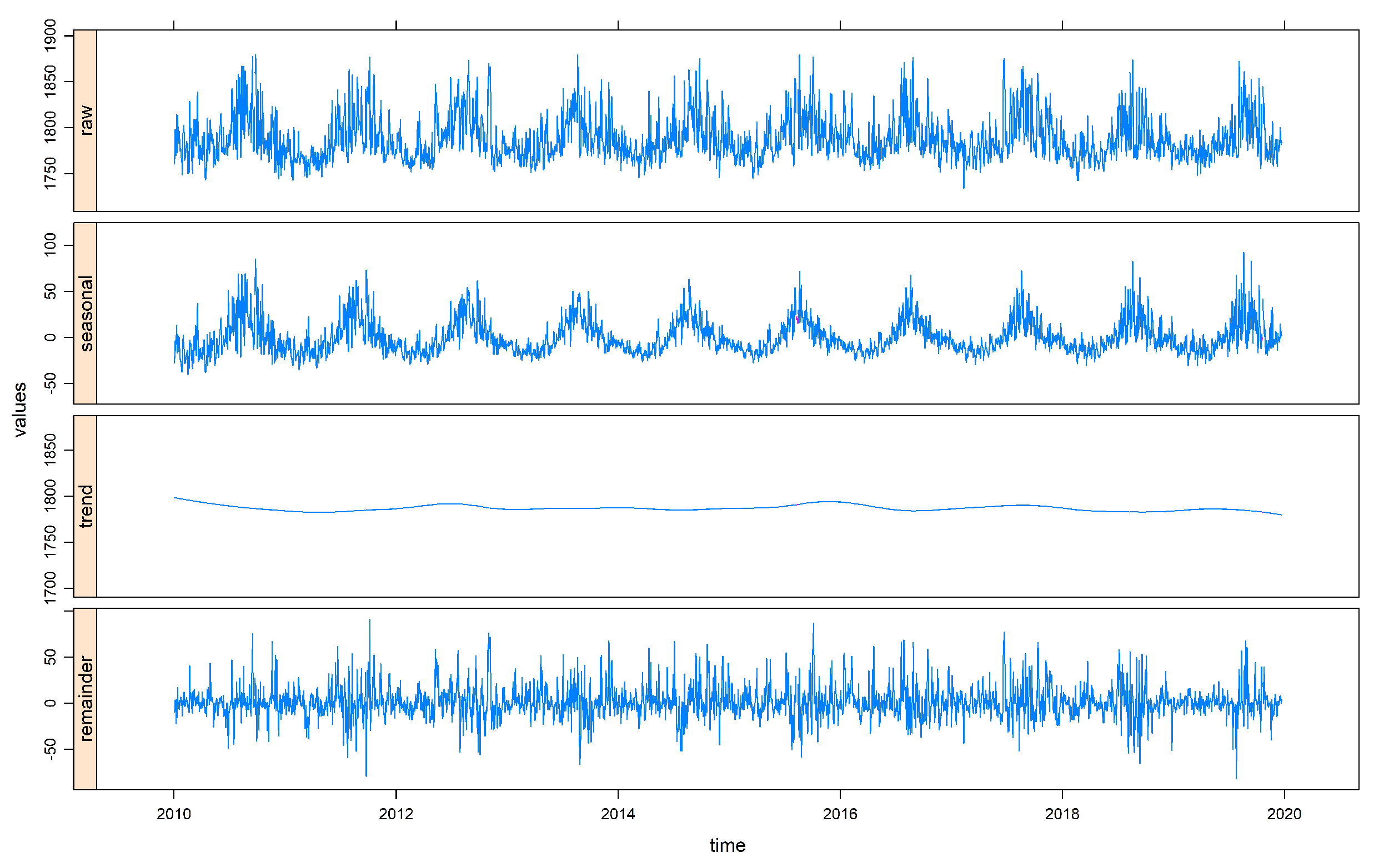
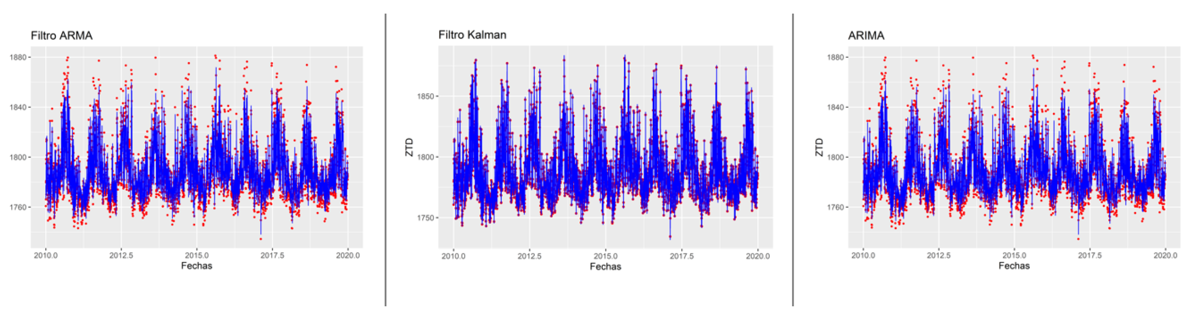
To give an idea of the behavior of the series, the corresponding results of applying the methodology, previously described, for the IZAN station in the time interval 2010–2020 are visualized, thus eliminating the possible influences that have occurred in the troposphere due to the volcano of La Palma, and, due to its location, the influence of the submarine volcano of El Hierro is also eliminated [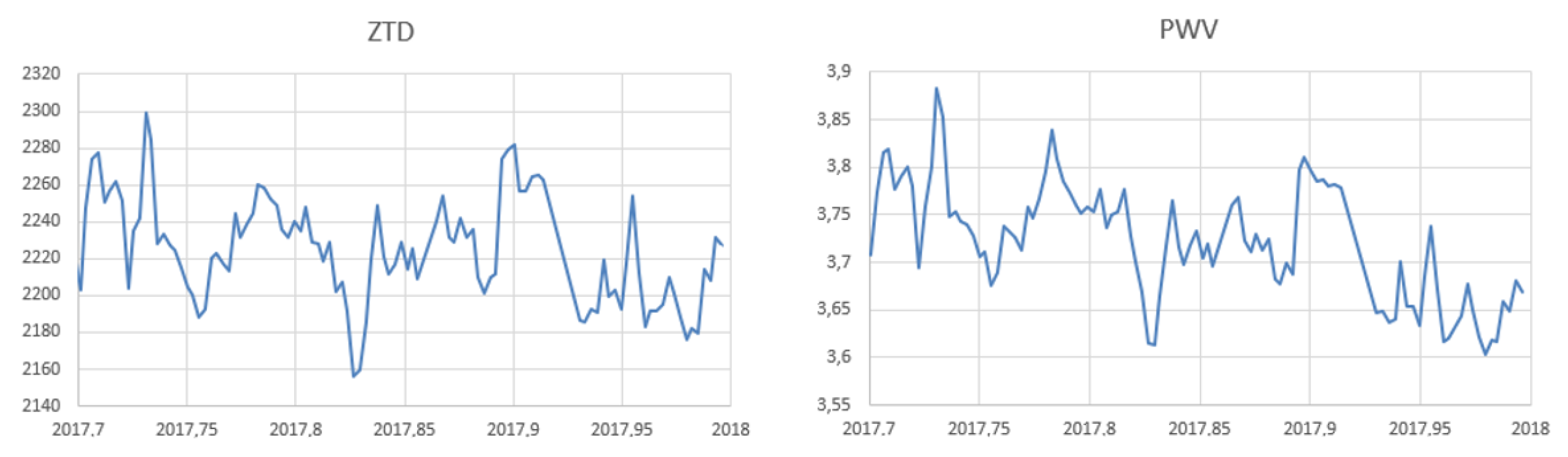15]. In addition, the graphs of the ZTD and PWV values corresponding to the EH01 station from September 2017 to 2018 will be shown.

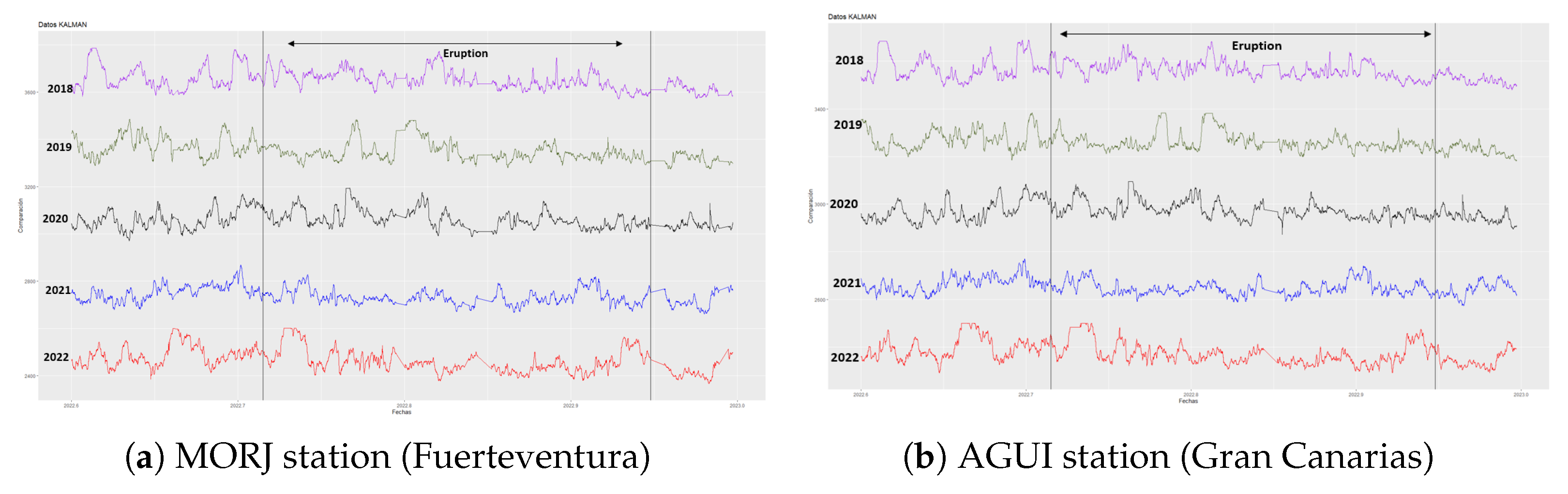
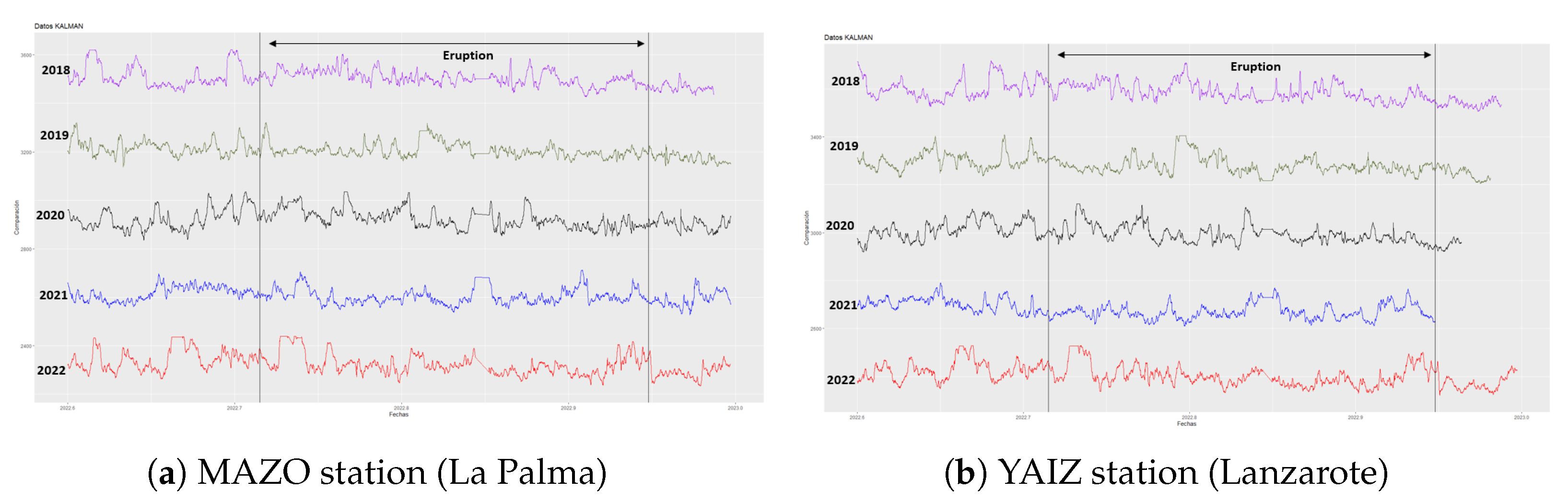
The ARIMA, ARMA, and Kalman methods will be applied to the permanent stations mentioned above, thus comparing the results obtained from each of the applied techniques, and the comparison between the ZTD and TEC values during the period from August to December in the years 2018, 2019, 2020, 2021, and 2022, marking the eruptive period in each of the years, the eruption occurring in the year 2021. A translation has been applied to these data to achieve an optimal visual comparison for the different years.

7. Conclusions

This paper seeks to know the influence that the eruption of the Cumbre Vieja volcano had on the ZTD and TEC values, for which the results obtained by applying the ARMA, ARIMA, and Kalman methods at different times have been analyzed. Observing the Figure 3 and Figure 4 shows the behavior without the volcanic influence of the IZAN station during the period 2010–2020. In both images, it can be seen that the data present a periodicity, after half the year it is seen how the time series grows, thus producing a seasonality that provides maximum points in the graph, which can be seen in the seasonal component that returns the STL decomposition. Figure 5 shows the comparison between the values of ZTD and PWV for station EH01 (El Hierro). 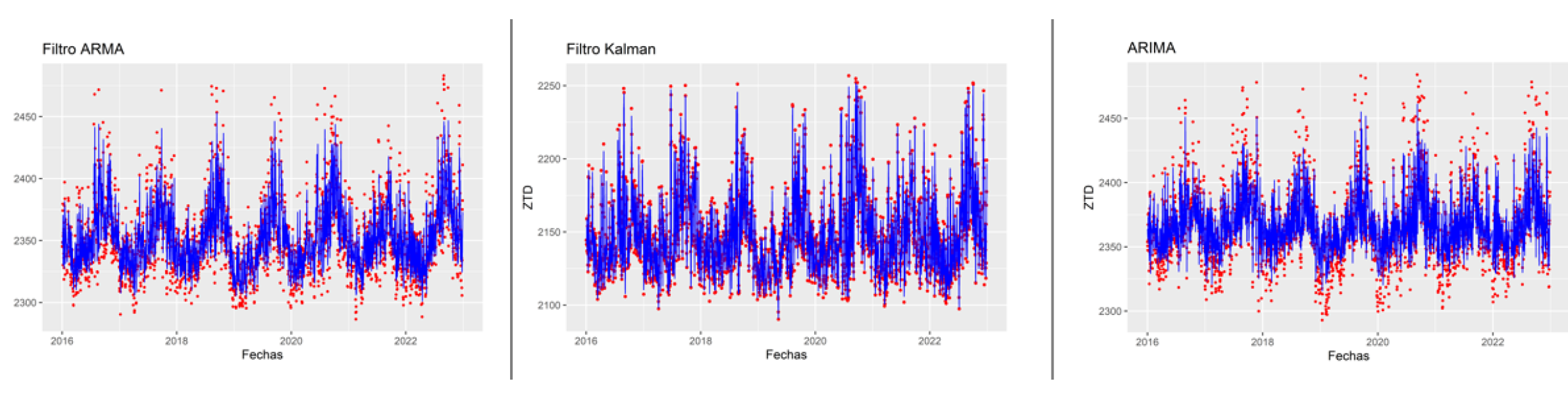Figure 6 shows the application of the ARMA, ARIMA and Kalman models for different stations. In the Figure 7 and Figure 8 obtained by comparing the methods during the months of August to December in the years 2018, 2019, 2020, 2021, and 2022, the data obtained by applying the various methods have been shown. A translation has been applied to these data to achieve a better visual comparison for the different years. It can be seen, as the data corresponding to the year 2021 are slightly more linear than the rest.

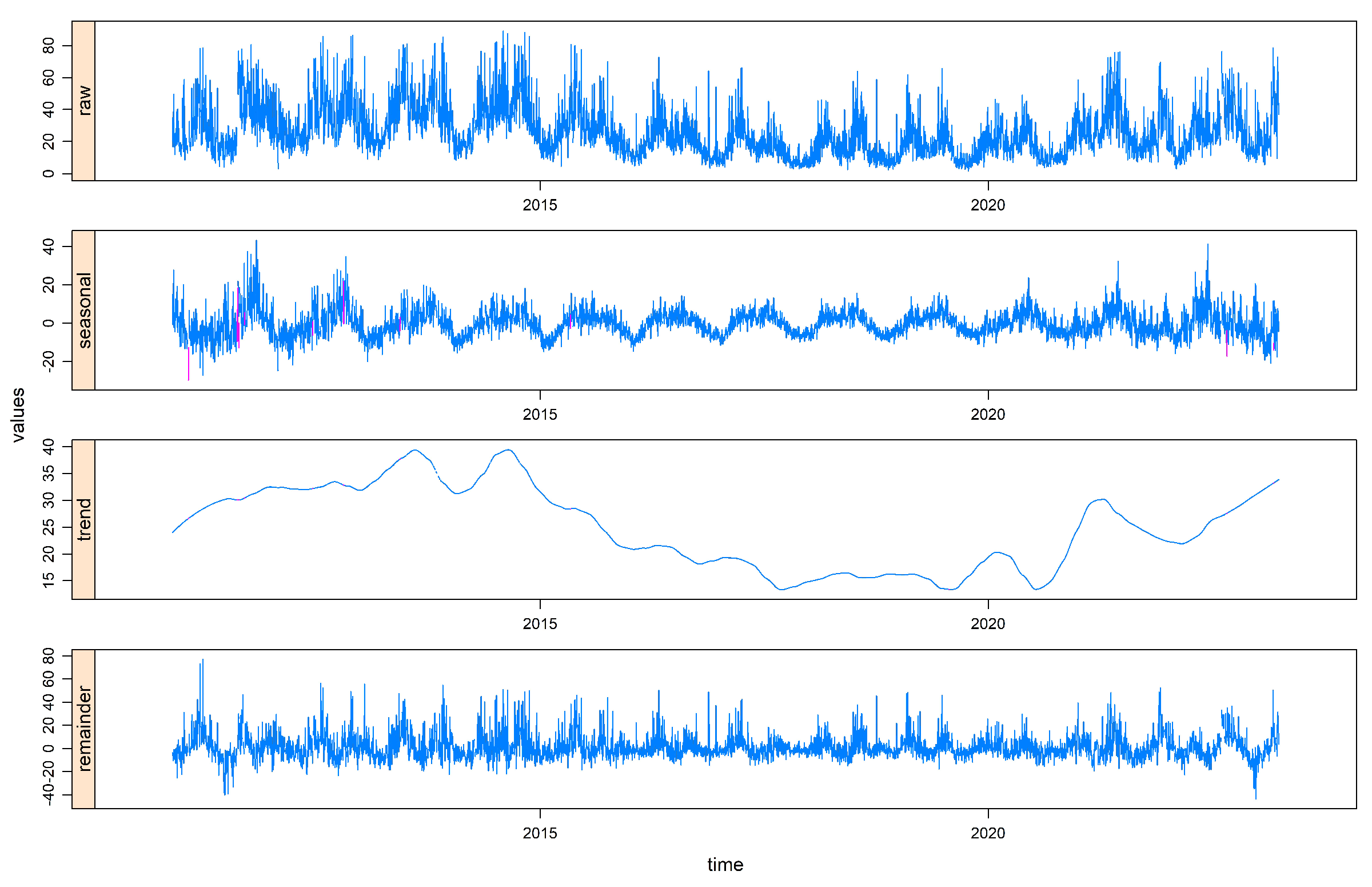
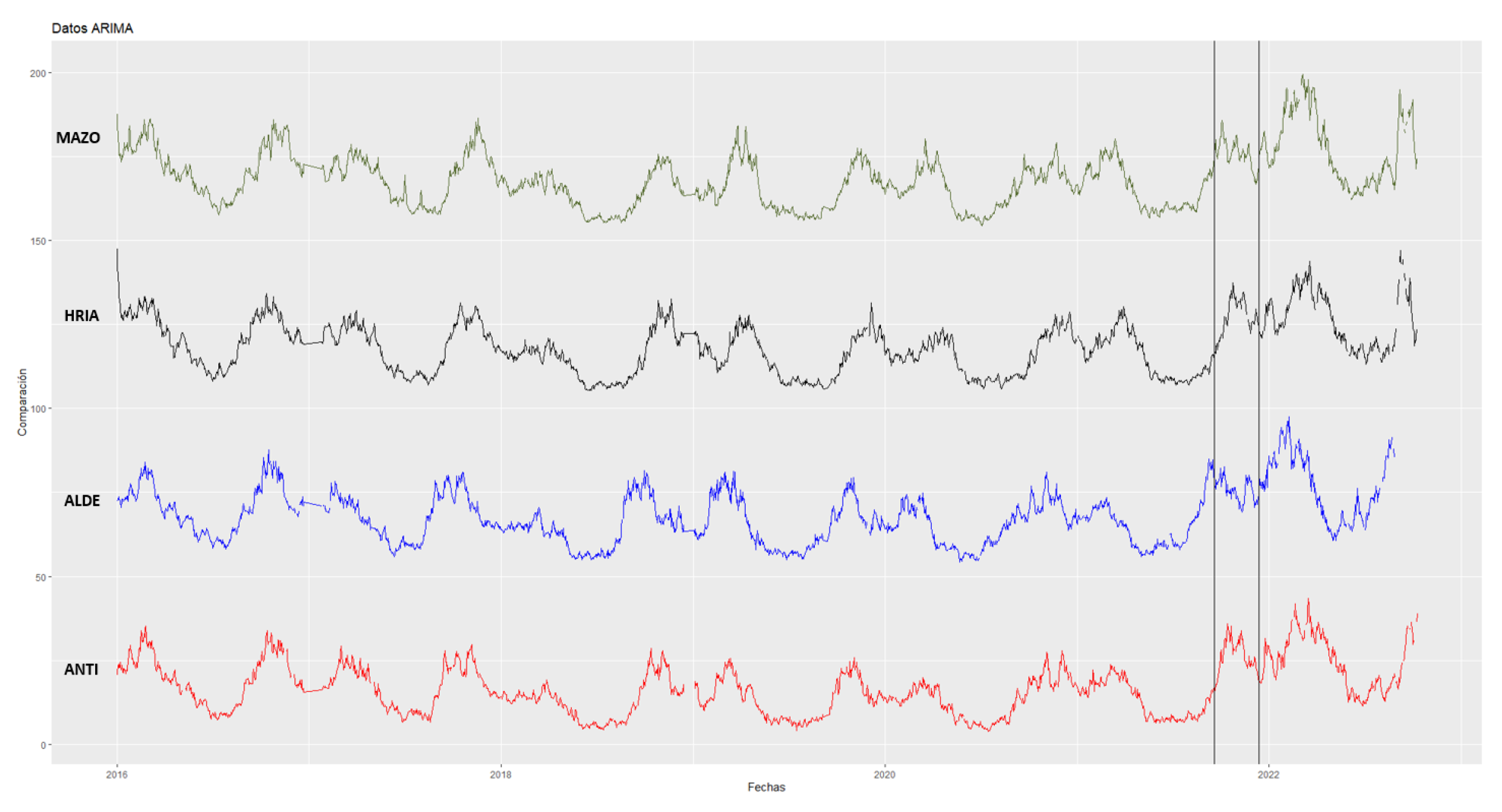
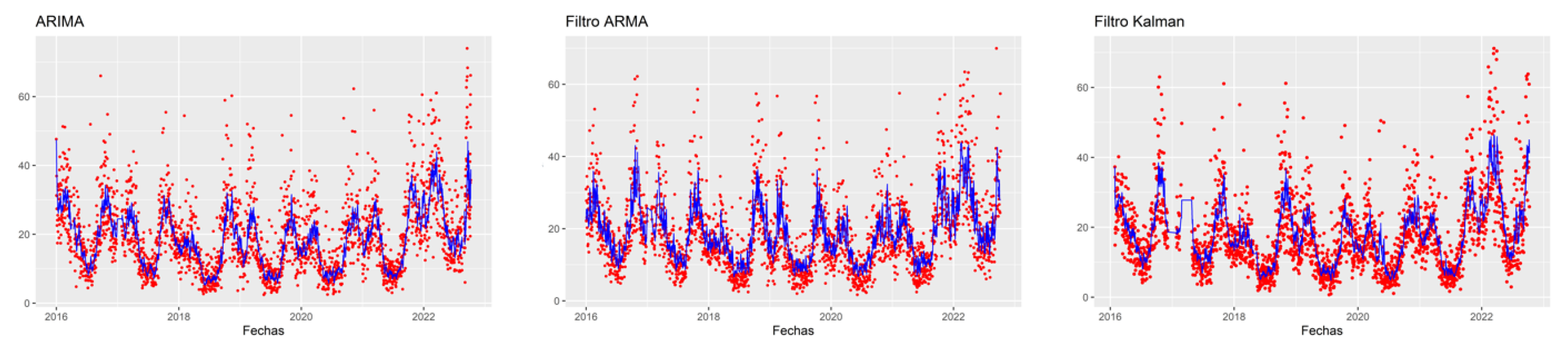
You can see the STL decomposition in Figure 9 for the TEC data, in the trend component the solar cycle that occurs every 11 years [2] is observed. In addition, Figure 9 shows the STL decomposition of MAZO (La Palma), in the seasonal component it can be seen that before 2022 the TEC values are higher. In Figure 10, the application of the ARIMA, ARMA models and the Kalman technique on the filtered data is shown. In Figure 11, there is a comparison of the ARIMA model for different stations with the dates on which the active volcano was marked; a rise can be seen during this period in the TEC values.

References

- Jin, S.; Jin, R.; Liu, X. GNSS Atmospheric Seismology; Springer: Berlin/Heidelberg, Germany, 2019. [Google Scholar]
- Dach, R.; Lutz, S.; Walser, P.; Fridez, P. Bernese GNSS Software Version 5.2. User Manual, Astronomical Institute, University of Bern, Bern Open Publishing, 2015; ISBN 978-3-906813-05-9. Available online: https://boris.unibe.ch/id/eprint/72297 (accessed on 14 April 2023).
- Gónzalez, Cárdenas, M.E.; Gosálvez, Rey, R.U.; Becerra, Ramírez, R.; Escobar, Lahoz, E. La Erupción de Cumbre Vieja de 2021; University of Castilla-La Mancha: Isla de La Palma, España, 2022. [Google Scholar]
- Sevilla de Lerma, M.J. Análisis de Series Temporales en Estaciones Permanentes GPS. Doctoral’s Dissertation, Universidad Complutense de Madrid, Madrid, Spain, 2015. [Google Scholar]
- Blewitt, G.; Hammond, W.C.; Kreemer, C. Harnessing the GPS data explosion for interdisciplinary science. Eos 2018, 99. [Google Scholar] [CrossRef]
- Barba, P.; Rosado, B.; Ramírez-Zelaya, J.; Berrocoso, M. Comparative Analysis of Statistical and Analytical Techniques for the Study of GNSS Geodetic Time Series. Eng. Proc. 2021, 5, 21. [Google Scholar] [CrossRef]
- Peña, D.; Peña, J. A normality test based on the Box-Cox transformation. Span. Stat. 1986, 33–46. [Google Scholar]
- Box, G.E.; Cox, D.R. An analysis of transformations. J. R. Stat. Soc. Ser. (Methodol.) 1964, 26, 211–243. [Google Scholar] [CrossRef]
- Martín Rodríguez, G. Representación en el Espacio de los Estados y Filtro de Kalman en el Contexto de las Series Temporales Económicas. Documentos de Trabajo Conjuntos: Facultades de Ciencias Económicas y Empresariales, Universidad de Las Palmas y Universidad de La Laguna, DT 2002/05. 2003, 5, 200246. Available online: https://accedacris.ulpgc.es/bitstream/10553/324/1/626.pdf (accessed on 14 April 2023).
- Prates, G.; García, A.; Fernández-Ros, A.; Marrero, J.M.; Ortiz, R.; Berrocoso, M. Enhancement of sub-daily positioning solutions for surface deformation surveillance at El Hierro volcano (Canary Islands, Spain). Bull. Volcanol. 2013, 75, 724. [Google Scholar] [CrossRef]
- Clevel, R.B.; Clevel, W.S.; McRae, J.E.; Terpenning, I. STL: A seasonal-trend decomposition. J. Off. Stat. 1990, 6, 3–73. [Google Scholar]
- Wu, M.; Jin, S.; Li, Z.; Cao, Y.; Ping, F.; Tang, X. High-precision GNSS PWV and its variation characteristics in China based on individual station meteorological data. Remote Sens. 2021, 13, 1296. [Google Scholar] [CrossRef]
- Aragón Paz, J.M. Estimación de paráMetros Troposféricos en Tiempo Casi Real para SUDAMérica Mediante téCnicas GNSS. Doctoral Dissertation, Universidad Nacional de La Plata, Buenos Aires, Argentina, 2020. [Google Scholar]
- Bevis, M.; Businger, S.; Herring, T.A.; Rocken, C.; Anthes, R.A.; Ware, R.H. GPS meteorology: Remote sensing of atmospheric water vapor using the Global Positioning System. J. Geophys. Res. Atmos. 1992, 97, 15787–15801. [Google Scholar] [CrossRef]
- Rosado, B.; Ramírez-Zelaya, J.; Barba, P.; de Gil, A.; Berrocoso, M. Comparative Analysis of Non-Linear GNSS Geodetic Time Series Filtering Techniques: El Hierro Volcanic Process (2010–2014). Eng. Proc. 2021, 5, 23. [Google Scholar]