Abstract
In time series analyses, the auto-regressive (AR) modelling of zero mean data is widely used for system identification, signal decorrelation, detection of outliers and forecasting. An AR process of order p is uniquely defined by p coefficients and the variance in the noise. The roots of the characteristic polynomial can be used as an alternative parametrization of the coefficients, which can be used to construct a continuous covariance function of the AR process or to verify that the AR process is stationary. In a previous study, we introduced an AR process of time variable coefficients (TVAR process) in which the movement of the roots was specified as a polynomial of order one. Until now, this method was analytically derived only for TVAR processes of orders one and two. Thus, higher-level processes had to be assembled by the successive estimation of these process orders. In this contribution, the analytical solution for a TVAR(3) process is derived and compared to the successive estimation using a TVAR(1) and TVAR(2) process. We will apply the proposed approach to a GNSS time series and compare the best-fit TVAR(3) process with the best-fit composition of TVAR(2) and TVAR(1) process.
1. Introduction
The auto-regressive process is a means in time series analysis and, among other things, this method is used to estimate discrete covariance functions (see [1] [p. 32, eq. (182)]) or to decorrelate observations by filtering [2,3,4]. Under the assumption of a non-stationary process, there are two possible states: first, that the roots of the characteristic polynomial are no longer in the unit circle, and therefore no covariances can be calculated, and secondly, the case we are looking at here, where the root changes over time, but always stays in the unit circle. This case has often appeared in the literature, but the TVAR coefficients, when used, were given a form of motion like polynomial motions (see [5,6]), trigonometric function [7], modified Legendre polynomials [8] and spherical sequences [9]. What all these methods often overlook is the resulting movement of the roots, as can be seen, for example, in [10]. In [11], it was derived how a TVAR process has to be calculated successively from TVAR(1) and TVAR(2) process estimates for a linear root movement. This method is now to be extended so that it can be applied directly to the TVAR(3) process without testing different series of TVAR(1) and TVAR(2) processes. Divided into five chapters, this extension is presented here. In Section 2, the necessary condition for the linear roots of a TVAR process of arbitrary order is derived again. In Section 3, additional restrictions are derived as sufficient conditions. In Section 4, the theory is tested on a GNSS time series and contrasted with successive estimations. The discussion of the results, as well as an overlook of further research directions, can be found in Section 5.
2. Successive Estimation Using TVAR(1) and TVAR(2) Processes
Ref. [10] defines the time variable auto-regressive process of the order p (TVAR (p) process) using the recursion formula
Here , , …, are the time-varying coefficients of the TVAR(p) process, and is an i.i.d. sequence with variance . As long as a single time is considered separately, the representation in (1) corresponds to a time-stable AR process of order p (TSAR(p) process):
According to [12] [p. 167], the TSAR Process is stationary if the roots (, , …, ) of the characteristic polynomial
are in the unit circle (∀). Ref. [11] has shown how TVAR processes with linear root movements are successively estimated using TVAR(1) and TVAR(2) processes, and the advantages of this method compared to the estimation of time constant AR processes. The general TVAR estimate consists of two steps: First, the coefficients of the TVAR process are replaced by polynomials, where the order of the polynomial is equal to the order of the coefficient
The general solution of can be calculated by a least squares adjustment using the system of equations
The order of the TVAR process is irrelevant for this calculation. Second, additional restrictions are put in place to ensure linear root movements. For orders 1 and 2, these restrictions were set out in the paper [11]. Now, this procedure is to be extended to the TVAR(3) process.
3. Restrictions of TVAR(3) Process with Linear Root Motion
The condition for the linear root movement arises from the transformation from the parameters () to the roots , respectively. Therefore, the representation of the roots from the coefficients for the time-constant case is considered first.
3.1. Calculation of the Roots from the Time-Stable Coefficients
The roots of a third-order polynomial
can be calculated after [13] [p. 22f] in a two-step procedure. The first step eliminates the monomial in (3) by substituting x with . For the resulting polynomial over y
the first roots of the Equation (4) can be determined using the Cardano solution:
where
This root is back-substituted to find the roots of the characteristic polynomial of the third order in (3):
The other two roots then result from
3.2. Restrictions for Linear Root Motion
These findings for a discrete point in time can be transferred to functions over time to derive the restrictions for linear root movements. However, this chapter does not derive the general condition for linear root motion; instead, the three sumands of
are individually converted into linear functions by restrictions. Because of the three conditions, all linear combinations of these functions (, and ) are automatically linear. This particularly applies to , and .
The conditions in (5), (6) and (7) have to be rewritten according to the conditions at the parameters . After the derivation of the coefficients in (2), is already a polynomial of first degree and the condition (7) is always met. To simplify the conditions in (5) and (6), both conditions are potentiated by 3 and then linked to each other via addition or multiplication:
This creates two new conditions: the first contains a third-order polynomial and the second a second-order polynomial, for which the equations are exactly satisfied if both sides have the same polynomial coefficients. Thus, the polynomial of order 3 in (8) includes four restrictions
and the polynomial of order 2 in (9) adds three further restrictions
4. Application: Two GNSS Time Series
To test the theory, the time series of an altitude component of a GNSS station (shown in Figure 1) is used. The data were provided by the Federal Institute of Hydrology (BFG), which operates a GNSS monitoring network for georeferencing and monitoring selected measuring stations.
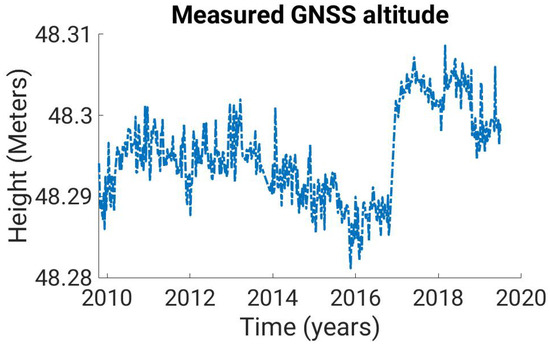
Figure 1.
A GNSS time series at the GNSS station in Pogum, Germany (TGPO) from end of 2009 to the begin of 2019.
Before the TVAR estimation can be performed, data jumps, data holes and trend must be removed from the observations. To eliminate the jump in the time series, all observations on the left side of the data jump are reduced by their mean value and the same is carried out for the right-side observations. The data gaps are interpolated by third-order splines. In order to establish the stationarity of the time series, each observation is reduced by its predecessor:
The offset of the resulting time series is eliminated by subtracting with the median of the time series. The result is shown in Figure 2.
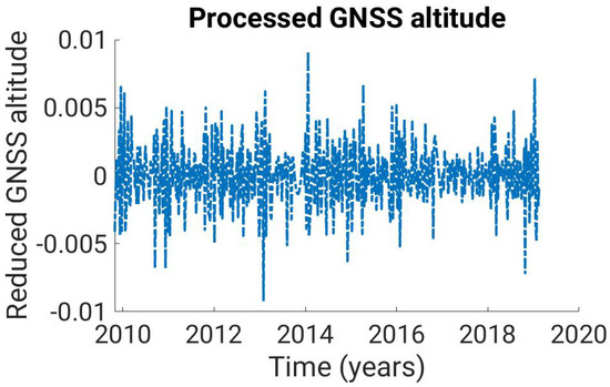
Figure 2.
Reduced time series . This is created from the time series by removing the data jump, extrapolating the data gaps and eliminating the trend.
In order to validate and compare the TVAR estimates later, we estimate time-stable AR(3) processes for a sliding window with the width of 100 observations. The roots of the AR(3) processes are shown in Figure 3. The time course goes from dark blue to light red, thus illustrating the temporal variability of the roots.
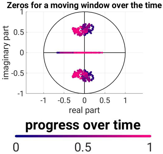
Figure 3.
The roots of stationary AR(3) processes from each 100 consecutive observations. Here, the same-colored points correspond to the evaluation of a window, and the color gradient represents the temporal assignment.
Now, the TVAR(3) process is estimated: On the one hand, this can be established via the direct method presented here for order 3 processes. The result is shown in Figure 4. Here, the linear movement of the roots is shown in the same color gradient as in Figure 3; the progress of the window had been displayed. For comparison, the roots from Figure 3 are shown as grey sequence in Figure 4 and Figure 5.
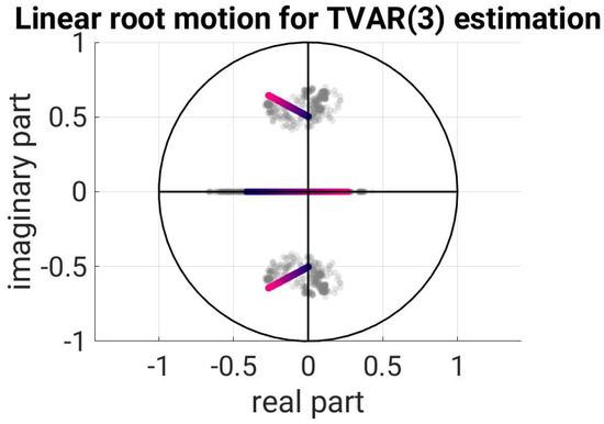
Figure 4.
Time course of the roots according to the direct TVAR(3) estimate.
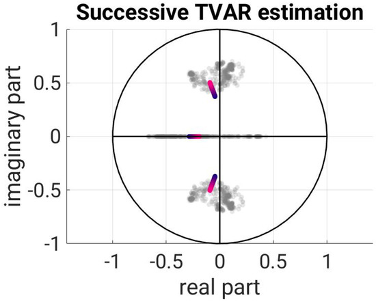
Figure 5.
Time course of the roots according to the best-fitted successive TVAR(3) estimate.
On the other hand, the successive estimation method from [11] was used to describe this time series. There are three ways to appreciate the TVAR(3) process:
- Via three TVAR(1) processes.
- Via a TVAR(1) process followed by a TVAR(2) process.
- Via a TVAR(2) process followed by a TVAR(1) estimate.
All three possibilities were realized and evaluated using the sum of squared residuals:
Here, is the error that occurs in the TVAR(3) estimation, and n is the number of errors per estimate. Method 3 had the smallest SSR, and was therefore used for the comparison. The resulting root movement is again contrasted with the result from the windowing and is shown in Figure 5.
In Figure 4, it can immediately be noted that the root motion of the direct calculation moves longitudinally through the roots of the windowing, while the roots of the successive estimation in Figure 5 show little movement and do not lie in the middle of the roots of the windowed version. Over time, the beginning and end points of the successive estimation are quite accurate in the first and last window, but the course of time is almost completely overlooked. The time course of the direct estimation has been approximated well by its counterpart.
5. Conclusions and Outlook
In this elaboration, a method has been developed which allows for TVAR(3) processes with linear root movements to be turned into estimates without sequential procedures. For this purpose, the TVAR(3) estimation was extended by three nonlinear conditions to obtain linear root motions. In an application, it was shown that the solution obtained by the direct estimation of a TVAR(3) process with linear root movements better fits the data than the successive estimation of TVAR(1) and TVAR(2) processes. Therefore, the method set out here shows a useful extension of the TVAR process estimation with linear root motions. In further studies, the conditions for the TVAR(4) process can be determined to expand the evaluation possibilities. Polynomial degrees higher than 4 are not possible. This follows from the realization that there is no way to analytically determine the roots for these polynomials (see [14]).
Author Contributions
Conceptualization, J.K.; methodology, J.K.; software, J.K.; validation, J.K., J.M.B. and W.-D.S.; formal analysis, J.K.; investigation, J.K.; resources, J.K.; data curation, J.K.; writing—original draft preparation, J.K.; writing—review and editing, J.K.; visualization, J.K.; supervision, W.-D.S.; project administration, W.-D.S.; funding acquisition, W.-D.S. All authors have read and agreed to the published version of the manuscript.
Funding
His research is funded by the Deutsche Forschungsgemeinschaft (DFG, German Research Foundation)—Grant No. 435703911 (SCHU 2305/7-1 ‘Nonstationary stochastic processes in least squares collocation—NonStopLSC’).
Institutional Review Board Statement
Not applicable.
Informed Consent Statement
Not applicable.
Data Availability Statement
Not applicable.
Conflicts of Interest
The authors declare no conflict of interest.
References
- Schuh, W.D. Signalverarbeitung in der Physikalischen Geodäsie. In Erdmessung und Satellitengeodäsie: Handbuch der Geodäsie, herausgegeben von Willi Freeden und Reiner Rummel; Rummel, R., Ed.; Springer Reference Naturwissenschaften; Springer: Berlin/Heidelberg, Germany, 2017; pp. 73–121. [Google Scholar] [CrossRef]
- Schubert, T.; Brockmann, J.M.; Schuh, W.D. Identification of Suspicious Data for Robust Estimation of Stochastic Processes. In Proceedings of the IX Hotine-Marussi Symposium on Mathematical Geodesy, Rome, Italy, 18–22 June 2018; Novák, P., Crespi, M., Sneeuw, N., Sansò, F., Eds.; Springer International Publishing: Cham, Switzerland, 2021. International Association of Geodesy Symposia. pp. 199–207. [Google Scholar] [CrossRef]
- Schuh, W.D.; Krasbutter, I.; Kargoll, B. Korrelierte Messung—Was Nun? In Zeitabhängige Messgrößen—Ihre Daten Haben (Mehr-)Wert; Neuner, H., Ed.; Wißner: Augsburg, Germany, 2014; Volume 74, pp. 85–101. [Google Scholar]
- Schuh, W.D.; Brockmann, J.M. Numerical Treatment of Covariance Stationary Processes in Least Squares Collocation. In Handbuch der Geodäsie: 6 Bände; Freeden, W., Rummel, R., Eds.; Springer Reference Naturwissenschaften; Springer: Berlin/Heidelberg, Germany, 2019; pp. 1–37. [Google Scholar] [CrossRef]
- Charbonnier, R.; Barlaud, M.; Alengrin, G.; Menez, J. Results on AR-modelling of Nonstationary Signals. Signal Process. 1987, 12, 143–151. [Google Scholar] [CrossRef]
- Kargoll, B.; Omidalizarandi, M.; Alkhatib, H.; Schuh, W.D. Further Results on a Modified EM Algorithm for Parameter Estimation in Linear Models with Time-Dependent Autoregressive and t-Distributed Errors. In Proceedings of the Time Series Analysis and Forecasting; Rojas, I., Pomares, H., Valenzuela, O., Eds.; Springer International Publishing: Berlin/Heidelberg, Germany, 2018; pp. 323–337. [Google Scholar]
- Grenier, Y. Time-Dependent ARMA Modeling of Nonstationary Signals. IEEE Trans. Acoust. Speech Signal Process. 1983, 31, 899–911. [Google Scholar] [CrossRef]
- Hall, M.; Oppenheim, A.V.; Willsky, A. Time-Varying Parametric Modeling of Speech. In Proceedings of the 1977 IEEE Conference on Decision and Control Including the 16th Symposium on Adaptive Processes and A Special Symposium on Fuzzy Set Theory and Applications, Tokyo, Japan, 7–9 December 1977; pp. 1085–1091. [Google Scholar] [CrossRef]
- Slepian, D. Prolate Spheroidal Wave Functions, Fourier Analysis, and Uncertainty—V: The Discrete Case. Bell Syst. Tech. J. 1978, 57, 1371–1430. [Google Scholar] [CrossRef]
- Kamen, E.W. The poles and zeros of a linear time-varying system. Linear Algebra Its Appl. 1988, 98, 263–289. [Google Scholar] [CrossRef]
- Korte, J.; Schubert, T.; Brockmann, J.M.; Schuh, W.D. On the Estimation of Time Varying AR Processes; International Association of Geodesy Symposia; Springer: Berlin/Heidelberg, Germany, 2023; pp. 1–6. [Google Scholar] [CrossRef]
- Dahlhaus, R. Fitting Time Series Models to Nonstationary Processes. Ann. Stat. 1997, 25, 1–37. [Google Scholar] [CrossRef]
- Ludyk, G. CAE von Dynamischen Systemen; Springer: Berlin/Heidelberg, Germany, 2013. [Google Scholar] [CrossRef]
- Ayoub, R.G. Paolo Ruffini’s Contributions to the Quintic. Arch. Hist. Exact Sci. 1980, 23, 253–277. [Google Scholar] [CrossRef]


Disclaimer/Publisher’s Note: The statements, opinions and data contained in all publications are solely those of the individual author(s) and contributor(s) and not of MDPI and/or the editor(s). MDPI and/or the editor(s) disclaim responsibility for any injury to people or property resulting from any ideas, methods, instructions or products referred to in the content. |
© 2023 by the authors. Licensee MDPI, Basel, Switzerland. This article is an open access article distributed under the terms and conditions of the Creative Commons Attribution (CC BY) license (https://creativecommons.org/licenses/by/4.0/).