Abstract
This paper analyzes how a robust and dynamic forecasting system was designed and implemented to predict material volumes for the inbound logistics network of an international automotive company. The system aims to reduce transportation logistics costs and improve demand capacity planning for freight forwarders. The forecasting horizon is set for 4 months and 12 months ahead in the future. To solve this problem, a time series modeling approach was carried out by using different time series forecasting methods like ARIMA, Neural Networks, Exponential Smoothing, Prophet, Automated Simple Moving Average, Multivariate Time Series, and Ensemble Forecast. Additionally, important data preprocessing methods and a robust model selection framework were used to train the models and select the best-performing one. This is known as Forward Chaining Nested Cross Validation with origin recalibration. The system performance was assessed using the Symmetric Mean Absolute Error (SMAPE). The final version of the forecasting system can deliver 4-month-ahead forecasts with a SMAPE lower than 10% for 86% of all material flow connections. The system’s forecast output is updated on a monthly basis and was integrated into the inbound logistics network system of the company.
1. Introduction
There are many business factors influencing a company’s performance. Among these, accurate forecasts have the greatest impact on an organization’s ability to satisfy customers and manage resources cost-effectively [1]. A forecast is not simply a projection of future business; it is a request for products and resources that ultimately impacts almost every business decision the company makes across sales, finance, production, management, logistics, and marketing [2]. An improvement in forecast accuracy, even just one percent, can have a ripple effect across the business, including reducing inventory buffers, obsolete products, expedited shipments, distribution center space, and non-value-added work [2].
Forecasting multiple time series can be challenging since every individual time series can display different properties. Some data might be trended, others might show seasonality. In other cases, data might just have random variations with underlying patterns which are hard to predict. Since there are different models whose properties better match up to particular time series characteristics [2,3,4], a common approach is to select the most effective and flexible models, blend their best features, and shift between them as needed to optimize forecast accuracy. Hence, enabling a forecasting system to automatically choose the best forecasting method over time is the best approach [2].
The current research considers an International Automotive Company that produces vehicles in more than 20 assembly plants around the world. The company currently has more than 1000 suppliers worldwide and more than 30 freight forwarders, which deliver different vehicle parts, components, and finished goods to their corresponding consolidation centers in the forwarding areas. To be precise, the company has an Area Forwarding-Based Inbound Logistics Network [5].
The increasing complexity in the Inbound Logistics Network, with regards to the production capacities from suppliers, the transportation availability from freight forwarders, and the changing materials demand from the assembly plants, have increased the need for reliable mid- and long-term capacity planning, especially for the freight forwarders. These are normally the actors in the logistics network with the lowest capacity and the less flexibility to abrupt planning changes. Therefore, a forecasting system focused on freight forwarders’ needs was set into place to predict inbound material transportation volumes from suppliers to plants.
Before the implementation of the forecasting system, there was a lack of synchronization between suppliers and freight forwarders, causing over- or under-capacity planning whenever a plant’s material demands change abruptly, leading to higher logistics transportation costs. Consequently, forecasting planning values delivered neither in the granularity nor in the frequency the freight forwarders expected.
The forecasting system has evolved since its creation in 2016. There have been three main Versions. Version 1.0 in 2016 which implemented five forecasting methods. Version 2.0 in 2018 implemented two additional forecasting methods, namely [6] and Multivariate Timeseries [7], as well as an automated outlier detection process [8] and a linear interpolation methodology [9]. Finally, Version 3.0 after the Coronavirus pandemic implemented further features related to improving production planning accuracy.
The system performance was assessed using the Symmetric Mean Absolute Error (SMAPE). Comparing the first and third versions, the system improved from 4-month-ahead to month-ahead forecasts with a SMAPE lower than 10% for 18% of all material flow connections, to a SMAPE lower than 10% for 86% of all material flow connections.
This paper is structured as follows: Section 2 points out the forecasting problem and explains the different strategies used in order to develop the forecasting system. Section 3 explains the forecasting system performance along the three versions. Limitations and further development are addressed in Section 4, and, finally, the conclusions are summarized in Section 5.
2. Materials and Methods
2.1. Business Problem Description
The realization of the forecasting system started with building an appropriate problem understanding together with the subject matter experts. Therefore, meetings with them were held in order to learn the most relevant characteristics of the logistic network, the data quality and availability, as well as the specific expectation of a forecasting system designed for the freight forwarders. From a methodological point of view, a time series approach was the most suitable tool since the problem comprises multiple hundreds of monthly time-related data. The system was developed using the programming language R.
The problem concerns the supply chain of an international automotive company with an Area Forwarding Inbound Logistics Network. This network consists of three major participants, (1) the assembly plant which has to be supplied with goods; (2) the suppliers which produce the material required by the plants. The suppliers are classified into groups, most likely regarding their geographical location. Such a group is called area forwarding. (3) Furthermore, the freight forwarder organizes the transportation of materials between the suppliers and the plants. In different areas, different freight forwarders can be hired by the same supplier. The freight forwarder operates a consolidation center within the area, collects goods from the suppliers, and gathers them in their consolidation center. This action is limited to cross-docking, i.e., there is no warehousing in the consolidation center. The pre-leg or first leg is the transportation step from the supplier to the consolidation center. At this point on, the goods from different suppliers in the area forwarding can be consolidated together. The transportation from the consolidation center to the assembly plants is called main leg transport. If the load in the pre-leg exceeds the volume of one vehicle, the materials are transported directly to the plants. This transportation type is called full truckload [5]. This network structure can be seen in Figure 1.
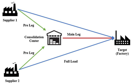
Figure 1.
Area Forwarding-based Inbound Logistics Network.
Syntetos’ Supply Chain Structure Framework is well known in the literature to help outline the components of a Logistics Supply Chain when it comes to forecasting [10]. Based on this framework, the company’s Inbound Logistics Network can be described as follows [1], (1) at the product dimension level the forecast regards all material components aggregated as tons; (2) at the location dimension it concerns all main leg material flows from the inbound material forwarding areas to the assembly plants; (3) at the time dimension forecasts are generated on a monthly basis for the next following 4 months and 12 months; and finally (4) at the echelon dimension the supply chain level corresponds to the material flows connections among the consolidation centers and the assembly plants.
2.2. Time Series Analysis
The project consisted of generating an adaptive and automated forecasting system for more than 400 main-leg material flows. Data were available on a monthly basis since 2014. The material flows display almost all possible demand patterns, i.e., positive and negative trends, seasonality, and irregular demand except for intermittent demand. Additionally, most of the time series contain outliers or missing values.
It is important to point out that a high correlation between the monthly production planning units and the monthly delivered material to the plants can be observed in the data. Another noticeable fact is that the monthly production planning forecasts are available up to 24 months into the future for every plant, giving an idea about how many vehicles are expected to be produced and how much material is expected to be delivered. Therefore, in order to make use of these data, rather than forecasting the monthly material volumes directly, a forecast of the ratio of material volume, and the production units (tons/vehicle units) is carried out:
This new time series is then referred to as time series (1). This is a smoother time series that is able to correct for outliers or extreme events in the material volumes. Finally, the business forecast in material tons is then given by the vehicle’s production forecast multiplied by the time series forecast. It is important to consider that since the vehicle’s production forecast is itself uncertain, its error is further propagated through the material volume forecast. This issue is addressed in version 3.0 of the forecasting system [11].
Regarding the error measures, the Mean Squared Error (MSE) was used to choose the best forecasting method in the model selection framework for a given material flow time series [4]. On the other hand, the Symmetric Mean Absolute Percentage Error (SMAPE) was used to evaluate the forecasts from the business perspective. Additionally, the SMAPE is a better estimator of the error than the MAPE when the true value of the forecast is close or equals zero since those tend to generate extremely large errors or infinite values [12]. Time series, with zero transported material volume, are common in this logistics network, and during the coronavirus crisis, it was even more likely to appear. When evaluating forecast accuracy, it is better to have different forecast error measures which can be then compared [4,13]. Therefore, the MSE was used to select the best-performing model; however, the interpretation from the business perspective and, therefore, the impact of the models will be analyzed using the SMAPE.
2.3. Model Selection Framework
According to the Logility Consulting Group [2], for many supply chain scenarios, it is best to employ a variety of methods to achieve optimal forecasts. Ideally, supply chain planners should take advantage of different methods and build them into the foundation of the forecast. The best practice is to use automated methods which switch to accommodate the selection and deployment of the most appropriate forecast method for optimal results. Henceforth, due to the nature of the problem, multiple models are evaluated and then the best-performing model on each material flow connection is selected to generate the monthly forecasts. To be precise, the Forward Chaining Nested Cross Validation with origin recalibration [4,14,15,16,17] method was implemented to carry out the model training and testing so that the best model can be chosen to generate the monthly forecasts. This method, explained in Figure 2, is able to replicate the data generation process so that the forecasting system learns in every iteration to select the best-performing forecasting algorithm; in consequence, it can dynamically adapt to short-term changes.
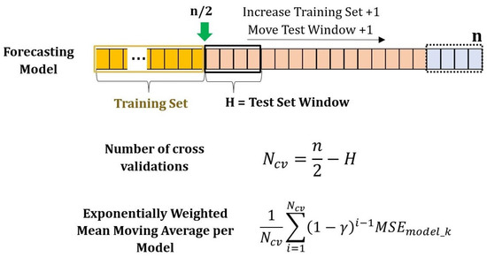
Figure 2.
Diagram of the Forward Chaining Nested Cross Validation with rolling origin recalibration described in [4,14,15,16,17].
A Nested Cross Validation approach provides an almost unbiased estimate of the true error of a model [17]. This refers to having two for loops in the train–test process; the inner for loop finds the best parameters estimates in the training set, then the outer for loop validates the true accuracy of the model using a rolling test window. Specifically, every time series, of n values, is split up into two sections, the training set and test set. Then, every model is fit using the training set and the best parameters are selected (inner for loop), then the model uses the best parameters to generate a forecast for the test window, and the MSE is calculated. Afterward, the training dataset increases by 1 value, and the test window is also moved 1 position into the future and the process is carried out repeatedly until no more test windows can be generated; this is called the literature forecast origin recalibration [16].
Due to the time dependency between the out-of-sample error measures of the cross-validation tests, a simple average of the resulting errors generates a biased indicator for choosing the best-performing model. Therefore, an exponential weighting approach can be applied to circumvent this problem [14]. The Exponentially Weighted Moving Average (EWMA) is a weighted average of all current and previous forecast errors, whose weights decrease geometrically with the “age” of the forecast error [4]. Therefore, the lowest resulting EWMA MSE is then used to select the best-performing model.
The resulting performance metrics are then stored in a database so that every month only the newest performance metrics for every material flow time series are added. This method enables the reduction in computing time and the forecast output for all the time series can be calculated in less than 30 min using a computer with 32 GB RAM and an Intel Core i7 Processor.
2.4. Forecasting System Version 1.0: First System Implementation
To create a forecasting system for monthly inbound material flows, first of all, meetings with the subject matter experts were held. From which the most relevant results were (1) the definition of the target variable, the monthly freight volume in tons; (2) the scope of the inbound logistics network, main legs; and (3) the forecast horizons, 4 months for mid-term and 12 months for long-term scenarios.
The subject matter experts pointed out the importance of including the production volume forecast as a feature in the forecasting process. For this, the time series transformation was implemented (see Equation (1)). This accounts for modeling the relationship between the monthly material flows in tons and the vehicles produced by each assembly plant and also the adjustment of extreme values in the times series. This is important since when outliers and missing values are incorrectly handled, they can certainly reduce the forecast accuracy [8,18].
Version 1.0 of the forecasting system was developed using the programming language R. The system focused on forecasting more than 400 main leg material flows within Europe. Furthermore, the model selection framework explained in Section 2 was also set up. This initial framework included the forecasting methods of Naive, ARIMA, Neural Network, Exponential Smoothing, and Ensemble Forecast. The last one refers to the average of the forecasts delivered by the other methods [19].
2.5. Forecasting System Version 2.0: New Forecasting Methods
Version 2.0 of the forecasting system implemented three additional forecasting methods to improve the forecast accuracy, namely Prophet Algorithm, Automated Simple Moving Average, and Multivariate Timeseries Method: Vector Autoregression.
The Prophet Algorithm from Facebook displays two main features, (1) parameters can easily accommodate seasonality with multiple periods and let the analyst make different assumptions about trends, (2) as opposed to ARIMA models, the measurements do not need to be regularly spaced, and missing values do not need to be interpolated, e.g., from removing outliers [6].
On the other hand, there are also important features that are left out when only using univariate methods. For this, Multivariate Methods are able to consider lag–cross correlations among different time series [7]. This cross-correlation feature, along with the historical data, considers the influence of past values of a time series A on the future value of a time series B and vice versa. Since there are multiple suppliers delivering to the same plants, the material quantity delivered from one supplier is highly correlated with the material delivered by other suppliers. This means a relevant cross-correlation between these material flows connections exist and can be exploited by this method.
Furthermore, a simple but useful method still not considered is the Simple Moving Average. The Simple Moving Average is the best model for products whose demand histories have random variations, including no seasonality or trend, or fairly flat demand [2]. However, finding the optimal parameters can be time-consuming. Therefore, using the R package smooth can help automate this process.
Additionally, the Ensemble Forecast method, which considers the simple linear combination (simple average) of the forecast values from the other methods, can be also extended, i.e., the Prophet Algorithm, Simple Moving Average, and Multivariate Time Series can also be included in the linear combination so that the likelihood of better forecasts accuracy increases [20].
One additional issue was the elimination of some past values due to a database update to the main Enterprise Resource System (ERP) Database. This leads to incomplete time series. Enabling a linear interpolation algorithm to find the missing values instead of using the mean of the observations can also improve forecasting accuracy. Linear interpolation is easy to implement [18], this enables us to find missing values for the time series in short computing run time. This method is efficient and most of the time is better than non-linear interpolations for predicting missing values [9].
Furthermore, an automated outlier detection and cleaning method was added. A common approach to deal with outliers in a time series is to identify the locations and the types of outliers and then use intervention models [21]. There are some main important issues caused by outliers, i.e., (a) the presence of outliers might result in an inappropriate model, (b) even if the model is appropriately specified, outliers in a time series might still produce bias in parameter estimates and, therefore, might affect the efficiency of outlier detection. A typical problem found in this approach is that both the types and locations of outliers may change at different iterations of model estimation, and (c) some outliers may not be identified due to a masking effect. For problems (b) and (c), Chen and Liu [8] designed a procedure that is less prone to the spurious and masking effects during outlier detection and is able to jointly estimate the model parameters and outlier effects. The approach is to classify an outlier impact into four types, an innovational outlier (IO), an additive outlier (AO), a level shift (LS), and a temporary change (TC). This method can be easily implemented using the R package tsoutliers. The process starts with setting SARIMA models to the time series, then the automated outlier detection method is applied to these ARIMA models, which delivers the outliers and their corresponding adjusted value. These adjusted values are then used instead of the outliers and a newly adjusted time series is generated, which can be later used for model training.
2.6. Forecasting System Version 3.0: Production Accuracy Improvement
Version 3.0 of the forecasting system focused on reducing the impact of the coronavirus crisis and the chip crisis by means of handling the increased volatility of both the material flows and the production planning so that reliable forecast values can still be delivered.
According to (Gultekin et. al, 2022), one of the most important freight forwarders’ risk areas, caused by the COVID-19 pandemic, was demand fluctuation. The pandemic increased the volatility in supply chain demand planning, making it even harder to generate accurate forecasts [22]. In total, 68% of the respondents on a 1000-company survey made by Capgemini 2020 stated that they experienced difficulties in demand planning due to a lack of data on fluctuating demand [23]. Furthermore, the current chip crisis is also one of the most relevant disruptive factors in the automotive supply chain. Opposed to forecasts, vehicle sales quickly rebounded within just a few months after the pandemic. Henceforth, imperfect inventory planning caused chip shortages and unprecedented halted production cycles [24].
Due to the heavy increase in the demand planning variability [23] post-COVID-19 outbreak, the production forecast has become less reliable. As explained in Section 2, when calculating the material volume forecast, the approach is to multiply the production demand planning by the time-series forecast. This leads, however, to error propagation since the production demand planning is itself a forecast. Therefore, in order to reduce this effect in the monthly material forecasting system, an additional data preprocessing approach was implemented.
This approach is called Production Planning Error Deviation Adjustment and helps to reduce the error propagation [11,25,26]. Since the production planning forecast is updated on a monthly basis, a database of monthly historical production plans was created. In other words, not only the actual number of vehicles to be produced are available but also the planning values in the previous months. The database consists of the monthly production plans since February 2019.
The approach is quite straightforward. The idea is to track the deviation of an actual production quantity from the forecast values in the past. For example, a plant produced 1000 in December 2020. If the planning value for this particular month is traced back to the previous months, then in some months the planning value would be over 1000 and in others under 1000, due to the variability in demand planning, as well as other internal and external factors. In consequence, using historical data, the relative error deviation to the actual produced cars can be calculated. The month distance from the production planning month to the actual production month will be called lag or planning horizon. Henceforth, let the Relative Planning Error Deviation for a lag l be
where = Relative Planning Error for lag l, corresponds to the planning vehicles for lag l, and to the actual produced vehicles.
This metric can be interpreted as follows. A value greater than 1 indicates that the planning demand was higher than the actual demand, therefore it was a planning overestimation. The opposite is a lower planning value than the actual demand, which is considered a planning underestimation.
Thence, to track the most recent changes in production planning the is calculated for every actual month available for the planning horizons 1 to 12 for every plant. To that end, the mean for lag l for every plant can be computed as
where is the number of values which could be calculated for the lag l with the available planning data. If the for a given plant for is 1.09, it means that historically the production planning overestimates on average about 9% the number of vehicles to be produced. Henceforth, the planning value can be adjusted by this amount.
Using the properties of the expected value of , assuming that the realizations of these errors are independent and identically distributed, an adjusted value of the vehicle’s demand planning can be computed. Since the actual number of produced vehicles in a month v is a constant and the expected value of is estimated with the most recent planning value, then the actual number of produced vehicles can be estimated as:
This formula enables us to estimate the true value of v, which the resulting demand planning values are now used to calculate the future monthly volume forecasts.
Figure 3 shows the Relative Mean Error Deviation (Production Forecast/Production Actual) for 4 plants. As expected, the further the forecasting horizon, the lower the quality of the forecasting values. Therefore, using the proposed method helps adjust the production planning data quality, and the forecast error propagation in the forecasting system is reduced therewith.
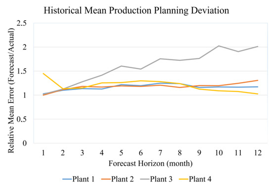
Figure 3.
Historical mean production planning deviation.
This was added as a data preprocessing step in the Forecasting System, enabling the future production demand planning values to be adjusted up to 12 months in the future.
3. Results
As pointed out in Section 2, the MSE was used to select the best-performing model. To analyze the business impact of the models, we used the SMAPE to compare model performance and improvement, since this enables a more straightforward interpretation of the error deviation. This section analyzes the performance of the forecasting system versions using the historically exponentially weighted moving average (EWMA) of the rolling 4-month-ahead out-of-sample SMAPEs. When comparing version A vs. version B, both systems’ versions were used to generate the forecasts for multiple months in the past using the same amount of data, then the EWMA is then calculated. With this, the EWMA-SMAPE Category distribution on the Material flow connections and the Cumulative EWMA-SMAPE Distribution is generated, as explained in the following sections.
3.1. Comparison Performance Version 1.0 vs. 2.0
The performance of the Forecast System Version 1.0 vs. Version 2.0 can be seen in Table 1.

Table 1.
EWMA-SMAPE Category Distribution on Material Flow Connections for Version 1.0 and 2.0.
To be precise, Table 1 shows the distribution of the EWMA SMAPE in groups. It is worth noting that the number of material flow connections with an EWMA SMAPE of less than 10% increased from 18.0% to 43.6%, i.e., about 25.6 pp (percentage points). Moreover, the number of material flow connections with an EWMA SMAPE higher than 40% decreased from 5.6% to 4.5%. Quantitatively, 80.1% of all material flows had an EWMA SMAPE of less than or equal to 20%, in comparison with the 66.7% of all material flows which had the same behavior when using version 1.0 of the forecasting system.
Regarding the different improvement steps carried out in version 2.0, Table 2 summarizes the results. The first column "Algorithms" presents the approaches used, whether it was a single forecasting method, a combination of multiple methods, or the implementation of data pre-processing steps. All tests were elaborated with the most recent data available at that moment. Furthermore, the column "Averaged EWMA SMAPE Improvement" shows the average percentage change for the EWMA SMAPE in the corresponding material flow connections selecting the new approach, which is found in the column "Material Flow Timeseries".
Table 2.
Improvement Results Forecasting System Versions 2.0 vs. 1.0.
First, the prophet algorithm was implemented; using the R package prophet [6]. This forecasting method showed an improvement of 9% in the material flows for monthly forecasts, with an average EWMA SMAPE improvement of 8.31%. Later, the algorithm Simple Moving Average (SMA) was introduced into the system. The function SMA from the R-Package smooth applies the Simple Moving Average method on a time series vector [27,28]. The SMA order was set to be chosen automatically by the function, which chooses the optimal one. In total, 24% of the material flows chose the SMA instead of the old methods. The average EWMA-SMAPE improvement was 3.78%.
For the implementation of the Multivariate Time Series, a vector autoregressive method was used. There are a couple of things which must be considered in advance. First, The Ljung-Box test is used to test the lag–cross correlation along n time series. The time series are divided into groups that are more likely to have the highest lag–cross correlation coefficient, namely, all the material flows coming to a single plant. Secondly, the automated vector autoregressive method might break down if too many time series with too few values are calculated. Explicitly, the algorithm takes up a large amount of memory and long runtime to calculate all the parameters involved in the matrices. Moreover, the number of lags consider to fit the model also affects the algorithm performance, which is why a 1-lagged automated vector autoregressive model was implemented in this case. Therefore, another routine was implemented to eliminate the parameters with a significance level lower than 5%. This step improved the model accuracy, as well as the final forecast errors. For this approach, 6.8% of the material flows realized a lower EWMA MSE cross-validation accuracy rather than using the old methods, that is an averaged EWMA SMAPE improvement of 23.78%.
Henceforth, the three new forecasting methods were tested together for all the material flow connections, for which, 42.8% of the connections displayed higher performance when choosing the new methods. This performance was translated into a 23.78% averaged EWMA SMAPE improvement in all four-step-ahead out-of-sample tests for data available.
Afterward, the data preprocessing methods were introduced. First, the automated outlier detection method together with the new forecasting algorithms was tested. These steps provided an improvement of 66.4% of the material flows with an average improvement for the EWMA SMAPE of 22.25%.
Later, the interpolation method for missing values was included delivering that 67.6% of the material flows chose the three new forecasting methods with an average improvement of 24.84% on the EWMA SMAPE. This can be seen in Figure 4. When plotting the cumulative EWMA SMAPE for all the material flow connections, the new forecasting system’s version shows a curve laying higher and more to the left of the graphic than version 1.0. This can be interpreted as more material flow connection forecasts displaying lower forecast errors.
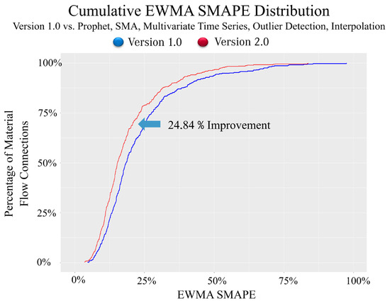
Figure 4.
Phase 1: EWMA MAPE comparison original forecasting system vs. improvements—Stand 2018.
Finally, from the company’s point of view, the SMAPE improvement has a greater impact on cost and demand capacity planning reduction when this is lower for material flow connections which transport on average more than 1000 tons monthly. Therefore, the logistics planners can better assess the forecasting system performance using a plot that shows the relationship between SMAPE performance and monthly average transported volume for every material flow connection. Figure 5 plots the average monthly material volume in tons and the EWMA SMAPE; every dot represents a material flow connection. From this plot, it can be implied that version 2.0 of the forecasting system delivered better results than version 1.0, in which almost all blue dots realized a lower four-month-ahead out-of-sample EWMA SMAPE than the red dots.
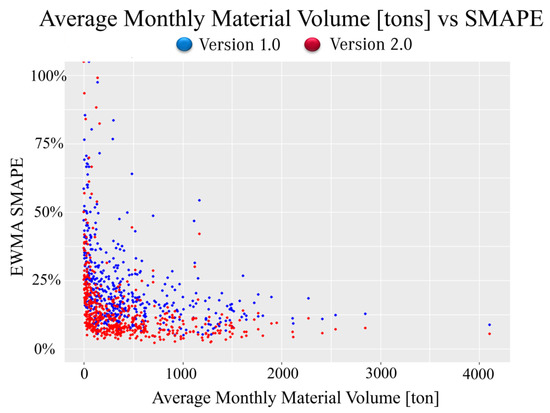
Figure 5.
Plot for Average monthly volume vs. EWMA SMAPE for Version 1.0 and 2.0.
3.2. Comparison Performance Version 2.0 and 3.0
The comparison of the Version 2.0 and Version 3.0 was carried out after the coronavirus crisis, at this time the structure of the inbound logistics network changed substantially, which is why the number of total material flows changed. The two versions of the system were assessed using new data, which is why the performance of Version 2.0 differs from that in the previous section.
The production accuracy improvement approach helped further improve the forecasting system. Considering that this approach traces the planning relative error deviation, future planning values are better estimated; thus, the monthly forecasts are more accurate. Table 3 summarizes the results after applying this methodology. When comparing the out-of-sample EWMA SMAPE values the new adjustment shows an improvement of 25.4% for material flow connections with an SMAPE lower than 10%. Furthermore, the number of material flow connections with a SMAPE greater than 40% was reduced from 2.7% to 0.2%. The major reason behind these improvements is due to two main factors, (1) the data input to the models uses the time series, which considers the historical production volume as an influencing factor; and (2) the final forecast is given by the production planning forecast times the time series forecast; the error propagation caused by the production planning is then highly reduced when applying the production accuracy improvement approach.
Table 3.
EWMA-SMAPE Category Distribution on Material Flow Connections for Version 2.0 and 3.0.
Finally, Figure 6 shows the performance of the forecasting system before and after applying this new approach, regarding the average monthly material volume and the SMAPE. It can be stated that the red dots representing the new forecasting system Version 3.0 realized a lower EWMA SMAPE over most material flow connections. Furthermore, material flow connections with more than 1000 tons on average also reached better performance, which can be directly translated into better performance planning in the inbound logistic network reducing logistic costs and capacity planning efforts.
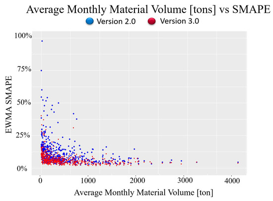
Figure 6.
Plot for Average monthly volume vs. EWMA SMAPE for Version 2.0 and 3.0.
4. Discussion
It was observed that after COVID-19, the prophet algorithm was the less recommended algorithm by the forecasting system; even in some months no material flow time series was predicted by it; i.e., the prophet algorithm was not capable of automatically adapting to the abrupt changes in the time series. This can be due to the decomposable time series model [6] in which the Facebook prophet is based, which resembles more than a mere curve fitting that does not take into account the conditional dependency of past realizations [29].
Further development of the forecasting system can be achieved by exploding the graph dependency structure of the data. Since capacity and production restrictions affect all plants, that means that future production capacity reductions in one plant can affect the production planning in another one. The use of most modern algorithms can help improve the forecasting accuracy and flexibility of the whole system. One proposed architecture is the use of Graph Neural Networks, which has been proven to successfully model graph-structured data [30].
5. Conclusions
The current research developed, designed, and implemented a monthly material flows forecasting system for the inbound logistics network of an international automotive company using multiple forecasting algorithms and robust data preprocessing routines. The system was also improved along with the changes in the market and adjusted to the company’s needs and challenges to deliver the highest forecasting accuracy, which was assessed using the Symmetric Mean Absolute Error (SMAPE). The output of the forecasting system was integrated into the inbound logistics system of the company delivering newly forecast values for the freight carriers on a monthly basis. This enabled the freight forwarders to better plan their capacities in the mid- and long-term (4-month-ahead and 12-month-ahead forecasts are delivered on a monthly basis) scenarios. Furthermore, the system supports the company by reducing logistics transportation costs and improving demand capacity planning since the material planning volume better meets the freight forwarder’s capacity.
Regarding the performance of the Forecasting System in the different versions; for 4-month-ahead forecast values, it can be seen that the number of material flows with an average EWMA-SMAPE of less than 10% increased through the different versions. From Version 1.0 to Version 2.0 the number of material flows with this performance increased from 18% to 43.6% (25.6 pp), whereas from Version 2.0 to Version 3.0 it increased from 60.3% to 85.7% (25.4 pp). This impact can be assessed using the Dupont Equation, which states that a 10% increase in forecasting accuracy can be translated into a return of shareholder value between 39% and 47% [2].
Furthermore, in the forecasting system’s versions 2.0 and 3.0, the methods having the highest impact on forecasting performance are those related to improving the data quality, i.e., the automated outlier detection procedure and the data interpolation method, which helped increase the impact of the three new algorithms from an average EWMA-SMAPE improvement of 7.8% of all material flow connections to 22.3%. In addition, the approach regarding production accuracy improvement helped increase the number of materials flows with an EWMA SMAPE of less than 10%. This result proves that when it comes to forecasting even the simplest method can deliver high performance if the quality of the input data is high enough.
The former assertion implies that the success of the forecasting system was not focused on the forecasting methods themselves but rather on the problem understanding, the data modeling, and the data preprocessing steps. Among these, we can highlight the use of the time series, the automatic outlier detection methods, and the error propagation correction for the production volume planning data. Enabling the system to robustly model the problem and adapt flexibly to upcoming supply chain disruption, not only from a mathematical but also from a business perspective, is the key to creating a highly performing forecasting system.
Author Contributions
Conceptualization, J.A.T.M. and A.K.; methodology, J.A.T.M., A.K., C.J.V.H. and E.L.A.; software, J.A.T.M. and A.K.; validation, J.A.T.M., A.K., C.J.V.H. and E.L.A.; formal analysis, J.A.T.M. and A.K.; investigation, J.A.T.M. and A.K.; resources, J.A.T.M.; data curation, J.A.T.M. and A.K.; writing—original draft preparation, J.A.T.M.; writing—review and editing, A.K., C.J.V.H. and E.L.A.; visualization, J.A.T.M.; supervision, A.K., C.J.V.H. and E.L.A. All authors have read and agreed to the published version of the manuscript.
Funding
This research received no external funding.
Institutional Review Board Statement
Not applicable.
Informed Consent Statement
Not applicable.
Conflicts of Interest
The authors declare no conflict of interest.
References
- Syntetos, A.A.; Babai, Z.; Boylan, J.E.; Kolassa, S.; Nikolopoulos, K. Supply chain forecasting: Theory, practice, their gap and the future. Eur. J. Oper. Res. 2016, 252, 1–26. [Google Scholar] [CrossRef]
- Logility. Eight Methods That Improve Forecasting Accuracy Eight Methods that Improve Forecasting Accuracy. Available online: https://www.logility.com/wp-content/uploads/dlm_uploads/2018/09/Eight-Methods-to-Improve-Forecasting-Accuracy-in-2019-Logility2019.pdf (accessed on 6 July 2023).
- Hyndman, R.J.; Khandakar, Y. Automatic Time Series for Forecasting: The Forecast Package for R. J. Stat. Softw. 2008, 27, 1–22. [Google Scholar] [CrossRef]
- Montgomery, D.; Jennings, C.; Kulahci, M. Introduction to Time Series Analysis and Forecasting; John Wiley & Sons: Hoboken, NJ, USA, 2008; p. 472. [Google Scholar]
- Schöneberg, T.; Koberstein, A.; Suhl, L. An optimization model for automated selection of economic and ecologic delivery profiles in area forwarding based inbound logistics networks. Flex. Serv. Manuf. J. 2010, 22, 214–235. [Google Scholar] [CrossRef]
- Taylor, S.J.; Letham, B. Forecasting at Scale. PeerJ 2017, 5, e3190v2. [Google Scholar] [CrossRef]
- Tsay, R.S. Multivariate Time Series Analysis with R and Financial Applications; John Wiley and Sons: Hoboken, NJ, USA, 2014. [Google Scholar]
- Chen, C.; Liu, L.M. Joint Estimation of Model Parameters and Outlier Effects in Time Series. JASA J. Am. Stat. Assoc. 1993, 88, 284–297. [Google Scholar] [CrossRef]
- Gnauck, A. Interpolation and approximation of water quality time series and process identification. Anal. Bioanal. Chem. 2004, 380, 484–492. [Google Scholar] [CrossRef]
- Punia, S.; Singh, S.P.; Madaan, J.K. A cross-temporal hierarchical framework and deep learning for supply chain forecasting. Comput. Ind. Eng. 2020, 149, 106796. [Google Scholar] [CrossRef]
- Lorenzato de Oliveira, J.F.; Pacífico, L.D.S.; Gomes de Mattos Neto, P.S.; Barreiros, E.F.S.; Rodrigues, C.M.d.O.; Filho, A.T.d.A. A hybrid optimized error correction system for time series forecasting. Appl. Soft Comput. 2020, 87, 105970. [Google Scholar] [CrossRef]
- Vladik, K.; Hung, T.; Nguyen, R.O. How to Estimate Forecasting Quality: A System-Motivated Derivation of Symmetric Mean Absolute Percentage Error (SMAPE) and Other Similar Characteristics; Technical Report: UTEP-CS-14-53; University of Texas at El Paso: El Paso, TX, USA, July 2014. [Google Scholar]
- Fildes, R.; Goodwin, P. Against your better judgment? How organizations can improve their use of management judgment in forecasting. Interfaces 2007, 37, 570–576. [Google Scholar] [CrossRef]
- Hjorth, U. Model Selection and Forward Validation. Scand. J. Stat. 1982, 9, 95–105. [Google Scholar]
- Bergmeir, C.; Benítez, J.M. On the use of cross-validation for time series predictor evaluation. Inf. Sci. 2012, 191, 192–213. [Google Scholar] [CrossRef]
- Tashman, L.J. Out-of-sample tests of forecasting accuracy: An analysis and review. Int. J. Forecast. 2000, 16, 437–450. [Google Scholar] [CrossRef]
- Varma, S.; Simon, R. Bias in Error Estimation When Using Cross-Validation for Model Selection. BMC Bioinform. 2006, 7, 91. [Google Scholar] [CrossRef]
- Lepot, M.; Aubin, J.-B.; Clemens, F.H.L.R. Interpolation in Time Series: An Introductive Overview of Existing Methods, Their Performance Criteria and Uncertainty Assessment. Water 2017, 9, 796. [Google Scholar] [CrossRef]
- Claeskens, G.; Magnus, J.R.; Vasnev, A.L.; Wang, W. The forecast combination puzzle: A simple theoretical explanation. Int. J. Forecast. 2016, 32, 754–762. [Google Scholar] [CrossRef]
- Smith, J.; Wallis, K.F. A simple explanation of the forecast combination puzzle. Oxf. Bull. Econ. Stat. 2009, 71, 331–355. [Google Scholar] [CrossRef]
- Box, G.; Tiao, G.C. Intervention Analysis with Applications to Economic and Environmental Problems. J. Am. Stat. Assoc. 1975, 70, 70–79. [Google Scholar] [CrossRef]
- Gultekin, B.; Demir, S.; Gunduz, M.A.; Cura, F.; Ozer, L. The logistics service providers during the COVID-19 pandemic: The prominence and the cause-effect structure of uncertainties and risks. Comput. Ind. Eng. 2022, 165, 107950. [Google Scholar] [CrossRef]
- Gya, R.; Lago, C.; Becker, M.; Junghanns, J.; Petit, J.-P.; Perea, L.; Schneider-Maul, R.; Dahlmeier, S.C.; Kumar, V.; Penka, A.; et al. Fast Forward Rethinking Supply Chain Resilence for a Post-COVID-19 World. Available online: https://www.capgemini.com/wp-content/uploads/2020/11/Fast-forward_Report.pdf (accessed on 6 July 2023).
- Alam, S.F.; Crean, S.; LeBlanc, J.; Naik, V. The Long View of the Chip Shortage: Building Resiliency in Semiconductor Supply Chains. Available online: https://www.accenture.com/_acnmedia/PDF-159/Accenture-The-Long-View-Of-The-Chip-Shortage.pdf (accessed on 6 July 2023).
- Liu, H.; Chen, C. Data processing strategies in wind energy forecasting models and applications: A comprehensive review. Appl. Energy 2019, 249, 392–408. [Google Scholar] [CrossRef]
- De Mattos Neto, P.; Cavalcanti, G.; Madeiro, F. Nonlinear Combination Method of Forecasters applied to PM Time Series. Pattern Recognit. Lett. 2017, 95, 65–72. [Google Scholar] [CrossRef]
- Svetunkov, I. Statistical Models UNDERLYING Functions of ’Smooth’ Package for R; Workingpaper; Lancaster University Management School: Lancaster, UK, 2017. [Google Scholar]
- Svetunkov, I.; Petropoulos, F. Old dog, new tricks: A modelling view of simple moving averages. Int. J. Prod. Res. 2017, 56, 1–14. [Google Scholar] [CrossRef]
- Seitz, S. Online: Facebook Prophet, COVID and Why I Do not Trust the Prophet. 2022. Available online: https://www-sarem–seitz-com.cdn.ampproject.org/c/s/www.sarem-seitz.com/facebook-prophet-covid-and-why-i-dont-trust-the-prophet/amp/ (accessed on 6 July 2023).
- Wu, Z.; Pan, S.; Long, G.; Jiang, J.; Zhang, C. Graph WaveNet for Deep Spatial-Temporal Graph Modeling. arXiv 2019, arXiv:1906.00121. [Google Scholar] [CrossRef]


Disclaimer/Publisher’s Note: The statements, opinions and data contained in all publications are solely those of the individual author(s) and contributor(s) and not of MDPI and/or the editor(s). MDPI and/or the editor(s) disclaim responsibility for any injury to people or property resulting from any ideas, methods, instructions or products referred to in the content. |
© 2023 by the authors. Licensee MDPI, Basel, Switzerland. This article is an open access article distributed under the terms and conditions of the Creative Commons Attribution (CC BY) license (https://creativecommons.org/licenses/by/4.0/).