Automata Based Multivariate Time Series Analysis for Anomaly Detection over Sliding Time Windows ^†

Abstract

We describe an optimal linear time complexity method for extracting patterns from sliding windows of multivariate time series that depends only on the length of the time series. The method is implemented as an open-source Java library and is used to detect anomalies in multivariate time series.

1. Introduction

Multivariate time series [1,2] are sequences or streams of more than one time-dependent variable corresponding to the simultaneous evolution of several variables over time. They can be observed in many areas and can thus be used to describe the evolution of key indicators.

Context. The analysis of time series makes it possible to extract certain behaviours that can be described by patterns [3]. These patterns inform us about the evolution of variables and provide trends observed in the time series. Patterns describing abnormal situations can be captured by regular expressions. The analysis of the time series consists of first identifying pattern occurrences in the time series, then associating a numerical value with each occurrence through the computation of a feature value. Anomaly detection then performs according to the following steps:

• Symbolically describe abnormal behaviours through patterns;
• Find the occurrences of these patterns in the time series;
• Identify the occurrences of those patterns whose numerical characteristics are deviant.

To identify these patterns, Beldiceanu et al. [3,4] used transducers, i.e., finite-state automata producing an output, which made it possible to efficiently identify pattern occurrences and calculate the corresponding feature value. This work and that of Arafailova [5] laid the necessary foundations for the development of our tool for detecting anomalies in time series.

Question addressed by this paper. The challenge is to design an efficient algorithm capable of identifying a succession of pattern occurrences denoting anomalies within the sliding time windows of a multivariate time series, where the patterns are described generically.

Our contribution. Given a multivariate time series with measurements over n instants and all sliding time windows over m consecutive instants, we describe an optimal time complexity algorithm in $\Theta \left(n\right)$ to identify all time windows containing occurrences of patterns corresponding to anomalies. A parameterised version [6] of this algorithm handling a variety of patterns was implemented as a Java library.

Paper organisation. In Section 2, we present the required background, such as patterns, features, and transducers. Then, in Section 3, we define the extraction of patterns occurrences on sliding windows; we present how patterns are evaluated both qualitatively and quantitatively using regular expressions and features. In Section 4, we present our anomaly detection tool and illustrate its use in Section 4.2 on environmental sensor data [7].

2. Background on Multivariate Time Series

A multivariate time series is obtained by observing the evolution of d measures over regular periods [8]. It is denoted as a n-dimensional array $\mathcal{X}=⟨X_1,X_2,\cdots ,X_n⟩$, where n is the length of the time series, d is the number of measures, $X_i\in {\mathbb{R}}^d$ is the i-th vector of measures, and $X_i^j$ is the j-th component of vector $X_i$. As a stream is unbounded, searching anomalies on a full stream does not make sense as data is generated continuously and sent in multiple data records; we rather want to identify anomalies on sliding windows of the stream [9]. Each window is a subsequence denoted by $X_{i,j}$ (with $i<j$) whose measures are defined from instant i to instant j. The next section shows how to describe conditions between two consecutive measures of a multivariate time series.

2.1. Alphabet as a Mean to Describe Conditions between Adjacent Measures

To specify patterns on a multivariate time series, the first step is to describe the basic elements of a pattern, namely a finite set of conditions between p consecutive measures of the time series. Each condition is interpreted as the letter of the alphabet $\Sigma$ that we now introduce.

Definition 1 

(alphabet). Given p consecutive measures $X_i,X_{i+1},\cdots ,X_{i+p-1}$, an alphabet Σ is defined as a set of mutually exclusive conditions $\{C_1,C_2,\cdots ,C_k\}$ such that $C_1\vee C_2\vee \cdots \vee C_k$ is true, where each condition $C_{\ell }$ (with $\ell \in [1,k]$) compares the components of $X_i,X_{i+1},\cdots ,X_{i+p-1}$ using the operators <, =, or >. Each condition $C_{\ell }$ of Σ must have its mirror condition $C_{\ell }^{mir}$ in Σ, where $C_{\ell }^{mir}$ is obtained by flipping the comparison operators < and > in $C_{\ell }$. Each of the conditions $C_1,C_2,\cdots ,C_k$ will be called a symbolic letter [10].

2.2. Signature of the Multivariate Time Series

The first step to analyse a multivariate time series $\mathcal{X}$ is to generate the sequence $\mathcal{S}$ of symbolic letters $S_i$ (with $i\in [1,n-p+1]$) associated with p consecutive measures of $\mathcal{X}$. This leads to the notion of signature $\mathcal{S}$.

Definition 2 

(Signature, arity). Consider a sequence of n measures $\mathcal{X}$ and a function  $\mathcal{F}:{\mathbb{R}}^p\to \Sigma$, where Σ is a finite set denoting an alphabet. Then, the signature of $\mathcal{X}$ is a sequence of symbolic letters $\mathcal{S}=⟨S_1,S_2,\cdots ,S_{n-p+1}⟩$ where each $S_i$ equals $\mathcal{F}(X_i,\cdots ,X_{i+p-1})$.

The alphabet $\Sigma$ is used to define regular expressions to symbolically characterise the occurrences of anomalies in $\mathcal{S}$. For this, we use patterns and features.

2.3. Pattern and Feature as Qualitative and Quantitative Aspects of Anomalies

The qualitative aspect of anomalies is described as the words of the language ${\mathcal{L}}_{\sigma }$ associated with the regular expression $\sigma$ defined over the alphabet $\Sigma$ [11].

Definition 3 

(Patterns [3]). A pattern σ over the alphabet Σ is a triple $⟨reg,b,a⟩$, where $reg$ is a regular expression over Σ that is only matched by non-empty words, while b and a are two non-negative integers, whose role is to delete parts of the pattern that are used to detect the start and end of a pattern.

Definition 4 

(Pattern reverse [4]). Two patterns $\sigma =⟨reg,b,a⟩$ and ${\sigma }^r=⟨re{g}^r,b^r,a^r⟩$ are the reverse of each other if $w_1{w}_2\cdots w_k\in {\mathcal{L}}_{\sigma }\iff w_k^{mir}{w}_{k-1}^{mir}\cdots w_1^{mir}\in {\mathcal{L}}_{{\sigma }^r}$, $a=b^r$, $b=a^r$.

A list of 22 patterns can be found in [4,12].

Features. After identifying a pattern occurrence in a time series, it is possible to characterise it with a numerical value. For this, we use features, which are functions allowing us to compute certain characteristics of a pattern occurrence, such as the min/max value. In [4], Beldiceanu et al. used five features for the quantitative evaluation of patterns in the context of sliding windows: one, width, surface, min, and max.

Aggregators. Sometimes, several occurrences of a pattern are identified in a sliding window. To obtain a unique result for the whole window, we use aggregators, which are functions that aggregate the features values on the different occurrences of the pattern. In [3,4], three aggregation functions are proposed: min, max,  and sum. In this paper, we only use the sumaggregator. To identify patterns occurrences in a time series, we use transducers.

2.4. Seed Transducers

Identifying pattern occurrences is achieved by using seed transducers [3]. We use deterministic finite transducers [13,14], which are automata $\mathcal{M}$ that generate an output sequence over the alphabet ${\Sigma }^{{}^{\prime }}$ from an input sequence over the alphabet $\Sigma$. To identify the occurrences of a pattern $\sigma$, our transducer reads one by one the symbolic letters $S_i$ in $\Sigma$ and triggers a transition from state $q_{i-1}$ to $q_i$ to produce a semantic letter ${\tau }_i$ in ${\Sigma }^{{}^{\prime }}$ associated with $S_i$. Each semantic letter designates a phase in the recognition of an occurrence of the pattern, e.g., when an occurrence of $\sigma$ is found, the semantic letter $\mathrm{FOUND}$ is generated. The semantic letter ${\mathrm{MAYBE}}_b$ means that the transducer has found the first letters of a potential occurrence of $\sigma$ but needs to read more letters to confirm it. The output alphabet ${\Sigma }^{{}^{\prime }}=\{\mathrm{OUT},{\mathrm{MAYBE}}_b$, ${\mathrm{OUT}}_r,\mathrm{FOUND},{\mathrm{FOUND}}_e,\mathrm{IN},{\mathrm{MAYBE}}_a,{\mathrm{OUT}}_a\}$ of a seed transducer is called the semantic alphabet. More details about their meaning can be found in [3].

Example 1. 

Let us consider a temperature and humidity measuring device that allows one measurement every hour. Our multivariate time series $\mathcal{X}$ is given in Table 1. Assume we want to identify the situation where, for two consecutive measures, i.e., $p=2$, both the temperature and the humidity increase. For this purpose, we define the alphabet $\Sigma =\{<,\le ,=,\ge ,>,\gtrless \}$ as:

$$\left\{\begin{array}{cc}<:\hfill & if{X}_i^1<X_{i+1}^1\wedge X_i^2<X_{i+1}^2\hfill \\ \le :\hfill & if(X_i^1<X_{i+1}^1\wedge X_i^2=X_{i+1}^2)\vee (X_i^1=X_{i+1}^1\wedge X_i^2<X_{i+1}^2)\hfill \\ =:\hfill & if{X}_i^1=X_{i+1}^1\wedge X_i^2=X_{i+1}^2\hfill \\ \ge :\hfill & if(X_i^1>X_{i+1}^1\wedge X_i^2=X_{i+1}^2)\vee (X_i^1=X_{i+1}^1\wedge X_i^2>X_{i+1}^2)\hfill \\ >:\hfill & if{X}_i^1>X_{i+1}^1\wedge X_i^2>X_{i+1}^2\hfill \\ \gtrless :\hfill & if(X_i^1>X_{i+1}^1\wedge X_i^2<X_{i+1}^2)\vee (X_i^1<X_{i+1}^1\wedge X_i^2>X_{i+1}^2)\hfill \end{array}\right.$$

Table 1. Multivariate time series $\mathcal{X}$: temperature and humidity level evolution over 17 h.

Time	1 am	2 am	3 am	4 am	5 am	6 am	7 am	8 am	9 am	10 am	11 am	12 pm	1 pm	2 pm	3 pm	4 pm	5 pm
Temp. (C)	19.3	21.5	19.2	21.4	23.6	22.8	22.8	20.1	20.9	21.5	22.7	23.6	23.6	19.2	21.5	21.5	21.5
Hum. (%)	74.9	52.2	74.8	52.1	73.2	72.3	65.7	55.9	52.1	64.5	64.5	72.7	62.4	59.8	52.1	55.2	55.2

We then define two patterns using the following observation. Normally, when the temperature increases, the humidity decreases and vice versa. Thus, when both metrics change in the same way (increasing or decreasing), it may be a sign of an anomaly. 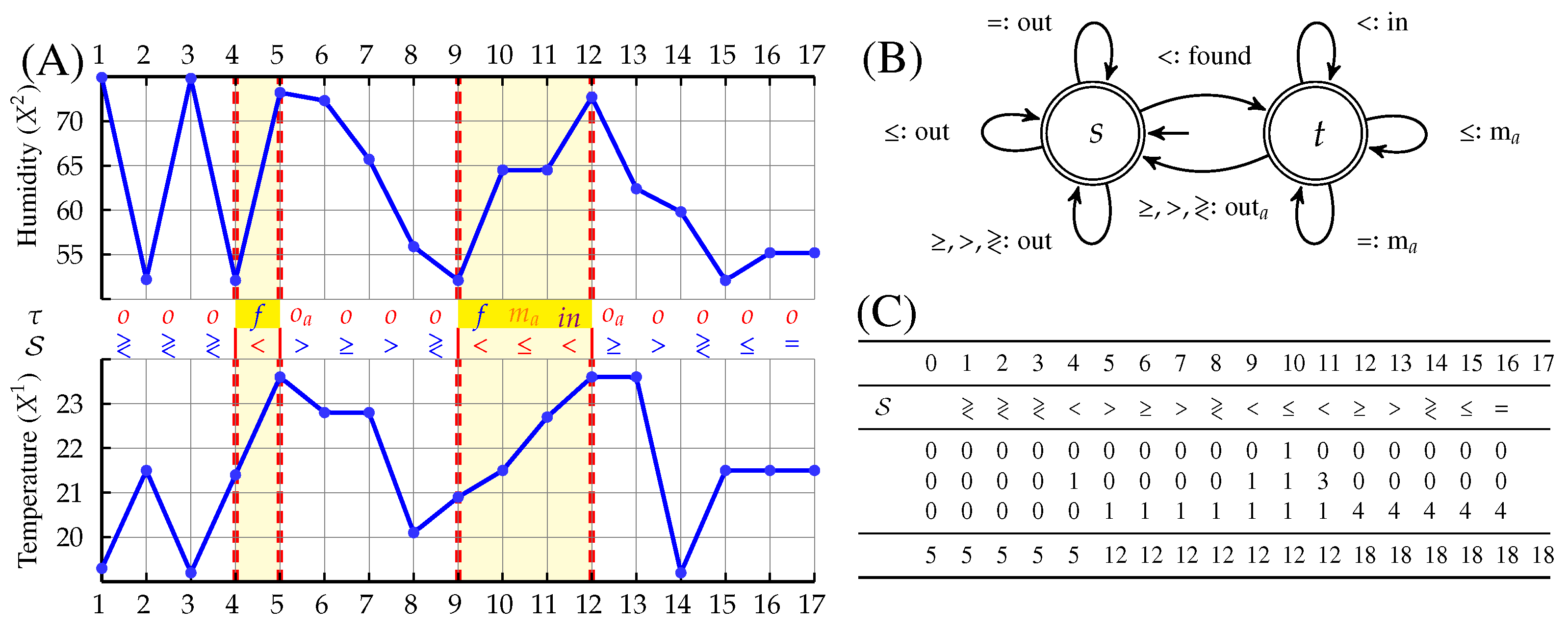These problematic changes are captured by the patterns and , respectively, corresponding to ${>|>(>|=|\ge )}^{*}>$ and ${<|<(<|=|\le )}^{*}<$, where describes a simultaneous decrease in both temperature and humidity, and an increase. Figure 1A shows two maximal occurrences of in the multivariate time series $\mathcal{X}$. Using the $\mathrm{W}\mathrm{IDTH}$ feature, we obtain $f_1=2$ and $f_2=4$ as the lengths of the two occurrences. Using the sumaggregator, we obtain a total length $g=6$. These values are computed using the transducer given in Figure 1B, which describes the transitions from the initial state s.

Figure 1. (A) Occurrences of pattern in a multivariate time series, (B) Transducer of pattern , (C) Accumulators updates.

3. Optimal Patterns Extraction from Sliding Windows

As explained in Section 2, the analysis of time series makes it possible to characterise them qualitatively with patterns, and quantitatively with features. The sum of the feature values of all pattern occurrences in a time series is called its contribution. We describe an optimal time-complexity algorithm for computing such contribution. This algorithm is used both when a multivariate time series corresponds to a single finite sequence of timed data, or when we have a data stream consisting of successive subsequences of timed data. Without lost of generality, we focus on a single finite sequence and show how to generalise it to a stream at the end of this section.

3.1. Register-Based Features Evaluation on a Time Series

Consider a multivariate time series $\mathcal{X}=⟨X_1,X_2,\cdots ,X_n⟩$, a pattern $\sigma$ and a feature f. To obtain the contribution of $\sigma$ on $\mathcal{X}$ we associate three accumulators $\mathrm{R}$, $\mathrm{C}$ and $\mathrm{D}$ to the transducer $\mathcal{M}$ of $\sigma$. We obtain a register automaton [3] in which each accumulator is updated as $\mathcal{X}$ is read:

• R gradually records the sum of the feature values of f on each completely terminated found occurrence of $\sigma$ (i.e., ${\tau }_i\in \{{\mathrm{OUT}}_a,{\mathrm{FOUND}}_e\}$);
• C stores the feature value of the current occurrence for which we did not yet reach the end (i.e., ${\tau }_i\in \{\mathrm{FOUND},\mathrm{IN}\}$);
• D contains the feature value of the current potential part of an occurrence (${\tau }_i\in \{{\mathrm{MAYBE}}_b,{\mathrm{MAYBE}}_a\}$).

Accumulators $\mathrm{R}$, $\mathrm{C}$, and $\mathrm{D}$ are updated according to the semantic letter ${\tau }_i$ returned by $\mathcal{M}$. Details of this evaluation can be found in [3,12].

Example 2 

(Continuation of Example 1). Reading $S_9=$ ‘<’ leads to ${\tau }_9=$ found. As shown in Table C of Figure 1, we then compute $\mathrm{C}\leftarrow \mathrm{D}+1$ (i.e., $C\leftarrow 1$), meaning that the length of the current occurrence of is 1. Similarly, ${\tau }_{10}=m_a$ means that we obtain a potential extra part of the already found occurrence of . We then compute its length with $\mathrm{D}\leftarrow \mathrm{D}+1$. ${\tau }_{11}=in$ means that we are still inside an occurrence of . It then confirms the membership of the encountered extra parts. Thus, we compute $\mathrm{C}\leftarrow \mathrm{C}+\mathrm{D}+1$. Finally, ${\tau }_{12}=o_a$ means that we are no longer in an occurrence of . We then compute $\mathrm{R}\leftarrow \mathrm{R}+\mathrm{C}$ to integrate $\mathrm{C}$ in $\mathrm{R}$.

3.2. Register-Based Features Evaluation on Sliding Windows

The contribution of a pattern on a sliding window $X_{i,j}=X_i,X_{i+1},\cdots ,X_j$ [15,16] is computed using Equation (1).

$$f_{\sigma }\left(X_{i,j}\right)=\left\{\begin{array}{cc}0\hfill & \mathrm{if}\mathrm{there}\mathrm{is}\mathrm{no}\mathrm{occurrence}\mathrm{of}\sigma \hfill \\ f_{\sigma }\left(X_{1,j}\right)+f_{{\sigma }^r}\left(X_{n,i}\right)-f_{\sigma }\left(X_{1,n}\right)\hfill & \mathrm{otherwise}.\hfill \end{array}\right.$$

(1)

Computing $f_{\sigma }\left(X_{i,j}\right)$ involves different steps. The first step consists of checking the presence of an occurrence of $\sigma$ in $X_{i,j}$, and the second step computes $f_{\sigma }\left(X_{1,j}\right)$, $f_{{\sigma }^r}\left(X_{n,i}\right)$, and $f_{\sigma }\left(X_{1,n}\right)$. In this section, we first show how to compute the contribution of $\sigma$ on $X_{1,j}$, then describe our method of identifying occurrences of $\sigma$ on sliding windows.

• Computing the Contribution of $\sigma$ on a Sliding Window 

In Equation (1), $f_{\sigma }\left(X_{1,n}\right)$ corresponds to the final value of $\mathrm{R}$ after reading $\mathcal{X}$ and $f_{\sigma }\left(X_{1,j}\right)$ to its value after reading the subsequence $X_{1,j}$. Similarly, $f_{{\sigma }^r}\left(X_{n,i}\right)$ corresponds to the value of $\mathrm{R}$ after reading the reverse sequence $X_{n,i}^r$ using the transducer of ${\sigma }^r$. To compute $f_{\sigma }\left(X_{i,j}\right)$, we first have to know the values of $\mathrm{R}$, $\mathrm{C}$, and $\mathrm{D}$ associated with each semantic letter returned. A first step is, therefore, performed to acquire the needed values exploited to optimally compute $f_{\sigma }\left(X_{i,j}\right)$.

• Pattern Occurrences Checker in Slidings Windows

To obtain an optimal time complexity algorithm, we also need to check whether each sliding window contains at least one pattern occurrence, i.e., see the first case of Equation (1). A naïve approach would be to check whether there is an occurrence of $\sigma$ in each window independently. Thus, considering a window size of m, the occurrence check of $\sigma$ on all sliding windows would lead to a time complexity of $O(m·n)$ [4].

To obtain an optimal time complexity of $\Theta \left(n\right)$, we create a new array, denoted as $\mathrm{E}$, which provides for each position in the time series, the end of the next occurrence of pattern in $\mathcal{X}$. Indeed, if there is an occurrence of $\sigma$ in $X_{i,j}$, then this occurrence will be defined between positions u and v, with $i\le u\le v\le j$. The accumulator $\mathrm{E}$ will indicate that an occurrence of $\sigma$ ends at v. Similarly, given that ${\sigma }^r$ and ${\mathcal{X}}^r$ are, respectively, the reverse of $\sigma$ and $\mathcal{X}$, then the end of an occurrence of ${\sigma }^r$ in ${\mathcal{X}}^r$ matches the start of an occurrence of $\sigma$ in $\mathcal{X}$ [4]. This makes it possible to say that an occurrence of $\sigma$ begins at u. The new accumulator $\mathrm{E}$ records at position k the end of the next occurrence of $\sigma$ from $X_k$. Table $\mathrm{C}$ of Figure 1 gives the values of $\mathrm{E}$ indicating the end of the next occurrences of in the multivariate time series $\mathcal{X}$ of Example 1.

• Computing the End of the Next Pattern Occurrence from the Pattern Transducer

Depending on the presence of found or found_e in the transducer $\mathcal{M}$, two cases must be distinguished:

-

When found_e $\in \mathcal{M}$, $\mathrm{E}$ is updated according to lines 3–9 of Algorithm 1;

-

When found $\in \mathcal{M}$, $\mathrm{E}$ is updated according to lines 10–20 of Algorithm 1.

In Algorithm 1, we use two types of assignments: value assignment, denoted ‘←’, and variable linkage, denoted ‘=’. For the first one, a value is directly assigned to a variable. For the second one, two variables are made equal using a linked list; when one of these variables is assigned, this assignment is automatically propagated to all the linked variables.

Linking two consecutive subsequences of a data stream. To find a pattern occurrence located across consecutive subsequences of a data stream, we use a buffer that records the last $m-1$ measures. Each new received sequence $⟨X_1,X_2,\cdots ,X_k⟩$ then integrates these past measurements as follows: $\mathcal{X}=⟨X_{-m+1},X_{-m+2},\cdots X_0,X_1,X_2,\cdots ,X_k⟩$.

Algorithm 1: Computing the end of the next occurrence of pattern for each position.

4. Anomaly Detection Tool

In this section, we describe an anomaly detection tool that exploits the efficient evaluation of patterns contributions on sliding windows. First, we give the key parameters of the tool. Then we present some experiments carried out.

4.1. Parameters

Anomaly detection is used to identify suspicious behaviour as data evolve. We use three parameters, namely: (i) the pattern $\sigma$ we are looking for, (ii) the feature f we consider, and (iii) the window size m. Anomalies occur when there are unusual values and when the sum of them exceeds a given threshold. We add two parameters to adjust the sensitivity of our tool to small variations in consecutive measures, and to multiple occurrences of unusual values:

• The minimum difference threshold ${\delta }_X$ is used to determine the minimum variation for two consecutive measures to be considered as different.
• The occupation percentage threshold $ϵ$ is the minimum percentage of the window occupation by the pattern wrt its contribution within the window. Thus, an anomaly is detected when the occupation percentage exceeds $ϵ$.

4.2. Experiments

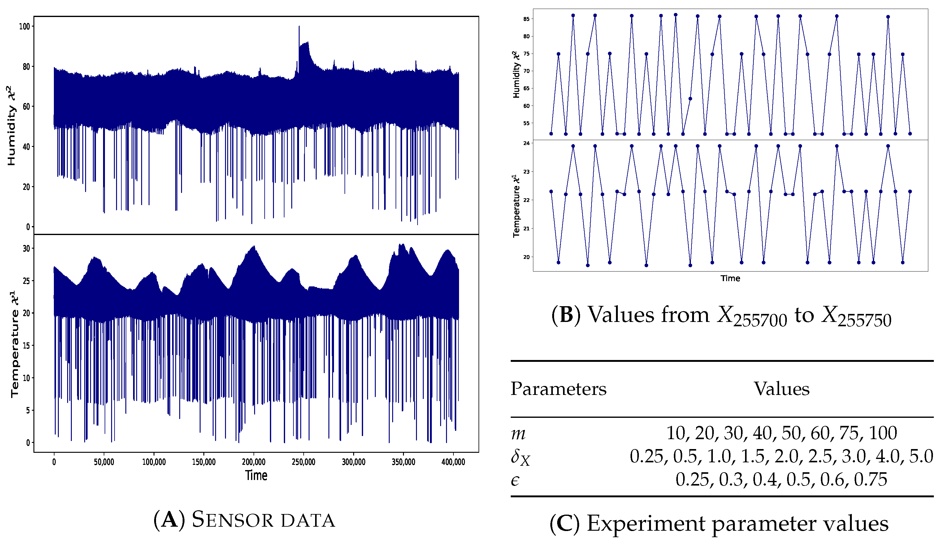
We have implemented our anomaly detection tools using Java 17. For the experiments, we analysed data from an environmental sensor [7]. These data show the evolution of temperature and humidity measurements over time, as shown in Figure 2. A visual analysis of Figure 2A highlights the existence of strong variations in the dataset with temperature or humidity, often dropping sharply to 0. A similar phenomenon can be observed with temperature increases of more than three degrees. Figure 2B gives a zoom-in and more detailed view of these variations. Each of these variations are potential anomalies that the tool identifies.

Figure 2. Evolution of the values of the analysed dataset and summary of the values of the parameters used in our experiments.

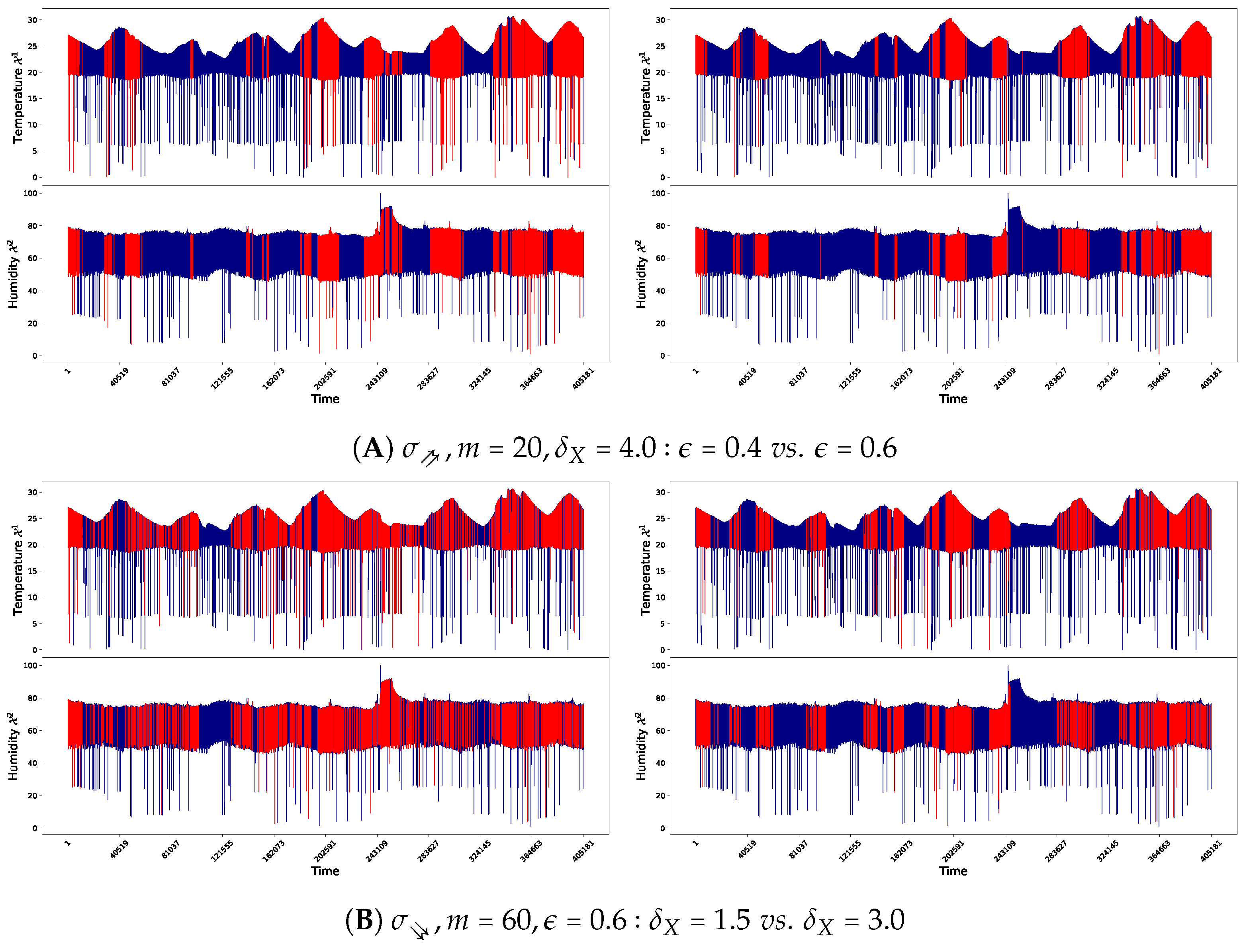
For our analysis, we used combinations of values of the previous parameters of Figure 2C. For all the combinations of values, we followed the following protocol: first, we identify problematic windows; second, we colour them in red and plot them; then we analyse the effects of each parameter variations. For space reasons, we will only show the results of two combinations of parameters, one for each of pattern and . The analysis of the results shown in Figure 3 then allows us to conclude that our tool allows one to efficiently identify anomalies occurrences in windows. The addition of parameters ${\delta }_X$ and $ϵ$, and the possibility of choosing the pattern to identify makes it possible to characterise the anomalies and to adjust their detection in a better way.

Figure 3. Problematic windows identified when using patterns and , and varying the values of ${\delta }_X$ and $ϵ$. These problematic windows are plotted in red, the non-problematic windows remain in blue.

• Effects of ${\delta }_X$ Variation

When analysing the effect of ${\delta }_X$ on the results, we notice that, as expected, small values of ${\delta }_X$ lead to the detection of more problematic windows. Indeed, large values of ${\delta }_X$ make it possible to ignore the small variations in the values of $X_k\in \mathcal{X}$ to consider only the large variations. Therefore, many, probably non-problematic occurrences of patterns are ignored. Conversely, with small values of ${\delta }_X$, these occurrences will be considered problematic and lead to more anomalies being detected. This behaviour is maintained whatever the pattern, the dataset or the values of m and $ϵ$.

• Effects of m and $ϵ$ Variation

The analysis of the effects of m and $ϵ$ shows that the bigger m is, the smaller must $ϵ$ be (and vice versa), if we want to catch a maximum number of problematic windows. Indeed, a large window size m may make it unlikely to find a high number of occurrences of $\sigma$. Therefore, the values of these two parameters should be adjusted inversely. This behaviour is maintained whatever the pattern, the dataset, or the values of ${\delta }_X$.

5. Conclusions

In this paper, we have proposed an efficient method for multivariate time series analysis. This transducer-based approach makes it possible to extract occurrences of patterns on sliding windows and to characterise them quantitatively with an optimal time complexity. We used the method for detecting anomalies and obtained a parameterised detection tool. The experiments we conducted show the ability of our approach to efficiently identify inconsistencies in data. In the future, we may consider other uses such as the automatic annotation of multivariate time series or the generation of time series.

References

- Audibert, J. Unsupervised Anomaly Detection in Time-Series. (Détection Non Supervisée des Anomalies Dans Les Séries Temporelles). Ph.D Thesis, Sorbonne University, Paris, France, 2021. [Google Scholar]
- Fawaz, H.I.; Forestier, G.; Weber, J.; Idoumghar, L.; Muller, P. Deep learning for time series classification: A review. Data Min. Knowl. Discov. 2019, 33, 917–963. [Google Scholar] [CrossRef]
- Beldiceanu, N.; Carlsson, M.; Douence, R.; Simonis, H. Using finite transducers for describing and synthesising structural time-series constraints. Constraints 2016, 21, 22–40. [Google Scholar] [CrossRef]
- Beldiceanu, N.; Carlsson, M.; Quimper, C.; Restrepo-Ruiz, M. Classifying Pattern and Feature Properties to Get a Θ(n) Checker and Reformulation for Sliding Time-Series Constraints. CoRR. 2019. abs/1912.01532. Available online: https://arxiv.org/abs/1912.01532 (accessed on 5 July 2023).
- Arafailova, E. Functional Description of Sequence Constraints and Synthesis of Combinatorial Objects. Ph.D. Thesis, IMT Atlantique, Nantes, France, 2018. [Google Scholar]
- Hien, A.; Beldiceanu, N.; Quimper, C.; Restrepo-Ruiz, M. Code and Supplementary Material. 2023. Available online: https://gitlab.com/postdochien/atisad (accessed on 5 July 2023).
- Stafford, G. Environmental Sensor Telemetry Data. 2020. Available online: https://www.kaggle.com/datasets/garystafford/environmental-sensor-data-132k (accessed on 5 July 2023).
- Morrill, J.; Fermanian, A.; Kidger, P.; Lyons, T.J. A Generalised Signature Method for Time Series. CoRR. 2020. abs/2006.00873. Available online: https://arxiv.org/abs/2006.00873 (accessed on 5 July 2023).
- Keogh, E.; Chu, S.; Hart, D.; Pazzani, M. Segmenting Time Series: A Survey and Novel Approach. In Data Mining in Time Series Databases; World Scientific: Singapore, 2004; Volume 57, pp. 1–21. [Google Scholar] [CrossRef]
- Veanes, M.; Hooimeijer, P.; Livshits, B.; Molnar, D.; Bjørner, N.S. Symbolic finite state transducers: Algorithms and applications. In Proceedings of the 39th ACM SIGPLAN-SIGACT, Philadelphia, PA, USA, 25–27 January 2012; pp. 137–150. [Google Scholar] [CrossRef]
- Crochemore, M.; Hancart, C.; Lecroq, T. Algorithms on Strings; Cambridge University Press: Cambridge, MA, USA, 2007. [Google Scholar]
- Arafailova, E.; Beldiceanu, N.; Douence, R.; Carlsson, M.; Flener, P.; Rodríguez, M.A.F.; Pearson, J.; Simonis, H. Global Constraint Catalog, Volume II, Time-Series Constraints. CoRR. 2016. abs/1609.08925. Available online: https://arxiv.org/abs/1609.08925 (accessed on 5 July 2023).
- Sakarovitch, J. Elements of Automata Theory; Cambridge University Press: Cambridge, MA, USA, 2009. [Google Scholar]
- Hopcroft, J.E.; Motwani, R.; Ullman, J.D. Introduction to Automata Theory, Languages, and Computation, 3rd ed.; Pearson International Edition: London, UK, 2006. [Google Scholar]
- Kolev, B.; Akbarinia, R.; Jiménez-Peris, R.; Levchenko, O.; Masseglia, F.; Patiño, M.; Valduriez, P. Parallel Streaming Implementation of Online Time Series Correlation Discovery on Sliding Windows with Regression Capabilities. In Proceedings of the 9th International Conference on Cloud Computing and Services Science, Heraklion, Crete, Greece, 2–4 May 2019; SciTePress: Setúbal, Portugal, 2019; Volume 1, pp. 681–687. [Google Scholar]
- Kontaki, M.; Papadopoulos, A.N.; Manolopoulos, Y. Adaptive similarity search in streaming time series with sliding windows. Data Knowl. Eng. 2007, 63, 478–502. [Google Scholar] [CrossRef]
Disclaimer/Publisher’s Note: The statements, opinions and data contained in all publications are solely those of the individual author(s) and contributor(s) and not of MDPI and/or the editor(s). MDPI and/or the editor(s) disclaim responsibility for any injury to people or property resulting from any ideas, methods, instructions or products referred to in the content. |
© 2023 by the authors. Licensee MDPI, Basel, Switzerland. This article is an open access article distributed under the terms and conditions of the Creative Commons Attribution (CC BY) license (https://creativecommons.org/licenses/by/4.0/).