Abstract
The study proposes an ensemble spatiotemporal methodology for short-term rainfall forecasting using several data mining techniques. Initially, Spatial Kriging and CNN methods were employed to generate two spatial predictor variables. The three days prior values of these two predictors and of other selected weather-related variables were fed into six cost-sensitive classification models, SVM, Naïve Bayes, MLP, LSTM, Logistic Regression, and Random Forest, to forecast rainfall occurrence. The outperformed models, SVM, Logistic Regression, Random Forest, and LSTM, were extracted to apply Synthetic Minority Oversampling Technique to further address the class imbalance problem. The Random Forest method showed the highest test accuracy of 0.87 and the highest precision, recall and an F1-score of 0.88.
1. Introduction
Rainfall is identified as one of the most chaotic and dynamic phenomena that varies spatiotemporally [1]. Heavy and extreme rainfall creates a serious threat to human lives and properties through severe flooding. Therefore, an accurate rainfall nowcasting is of great significance in preventing devastating consequences.
The data mining techniques optimally capture the hidden spatiotemporal patterns among largely available weather-related data [2]. Many researchers achieved high prediction accuracy in rainfall classification using techniques such as Random Forest, Artificial Neural Network (ANN), K—Nearest Neighbour (KNN) and Support Vector Machine (SVM). As a recent trend, deep learning methods such as Convolutional Neural Network (CNN) and Long-Short-Term-Memory (LSTM) are employed to explore the meteorological big data due to its promising technical advantages and performance [3]. The study performed in [4] used K-means clustering to predict rainfall states. The identified clusters were used as predictands for training the Classification and Regression Tree (CART) model with five climate input variables and obtained a satisfactory value of goodness-of-fit. Another study performed CART and C4.5 models with thirteen input variables to predict the chance of rain and gained average accuracies of 99.2% (CART) and 99.3% (C4.5) [5]. Moreover, [6] modeled weekly rainfall with weather variables using ANN and produced higher prediction accuracy than multiple linear regression model. The summer precipitation patterns over eastern China were modeled using multinomial logistic regression (MLR) by [7] and gained a prediction accuracy range of (60–70%). Authors of [8] compared several machine learning models in classifying month of a year as dry or wet. The rainfall classification carried out by [9] concluded that Decision Trees and Random Forests could perform well even with a low proportion of training data. A similar study conducted by [10] extracted the Adaboost algorithm, which produced F1-score of 0.9726. Authors of [11] carried out rainfall classification addressing the class imbalance through over and under-sampling techniques, and the results indicated varying performance with different inputs generated by resampling techniques.
Our study employed several cost-sensitive machine learning models, including Penalized SVM and Complement Naïve Bayes followed by a resampling technique to address the natural rarity of extreme rainfall events. Prior to that two spatial input variables were generated by modeling satellite data with deep learning method (CNN) and rainfall at nearby rain gauging stations with Spatial Kriging. Therefore, the study focused on three solutions proposed by the literature [12] for imbalance learning. Moreover, we have performed a comparative study between machine learning and deep learning models suggested by many researchers [11,12].
2. Materials and Methods
2.1. Description of Data
The weather data was obtained from the Meteorology Department of Sri Lanka based on the Kalu River basin over the period from 2015 to 2019. It includes daily data on 28 variables including rainfall at target rain gauging station (Rathnapura), rainfall of six nearby gauging stations, relative humidity, mean sea level pressure, wind speed, temperature, sunshine hours, evaporation, and Southern Oscillation Index. Additionally, the study collected daily satellite images (with a size of 500 × 512 pixels) covering the river basin from China Meteorological Administration National Satellite Meteorological Center for the same time period.
2.2. Methods
The main objective of the study is to forecast rainfall occurrences from highly imbalanced spatiotemporal time series data by using machine learning and deep learning methods. Initially, the rainfall classes needed to be identified. Therefore, with the cutoff levels established by Meteorology Department of Sri Lanka and a comparison of flood occurrence with respect to rainfall at Rathnapura, the rainfall values were categorized into three classes, ‘No rainfall’, ‘Normal rainfall’, and ‘Extreme rainfall’. Following the norm of the Department of Meteorology, Sri Lanka, the cutoff level for extreme events was set at 110 mm of rainfall. Then, the methodology illustrated in Figure 1 was carried out.
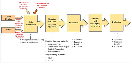
Figure 1.
Ensemble Spatiotemporal Data Mining Approach.
The Spatial Kriging was applied to predict current day (t) rainfall at Rathnapura using current day rainfall values of six nearby stations to incorporate spatial correlation between nearby stations and target station to final model. The previous day (t − 1) satellite image was modeled to predict the current day (t) rainfall class through CNN model. Then, the predicted rainfall class of the day t with the predicted rainfall value of the same day were brought as predictor variables to the final dataset along with other selected variables. The values of these predictor variables of last three consecutive days (t, t − 1, t − 2) were fed into six classifiers from different model families (Linear Classifier, Ensemble, and deep and sequential learning) for forecasting next day (t + 1) actual rainfall class of target variable or the response variable.
2.2.1. Spatial Kriging
Let the rainfall value in Rathnapura on a particular day be . In Spatial Kriging estimates of , is modeled through the rainfall values of neighboring sample locations , i.e., . It gives an optimal linear combination of with weights , which are taken according to covariance values [13].
2.2.2. Multi-Layer Perceptron (MLP)
MLP is a feed forward neural network that consists of three types of layers, the input layer, hidden layer (s), and output layer [14]. Let us consider a MLP model (see Figure 2) with one hidden layer.
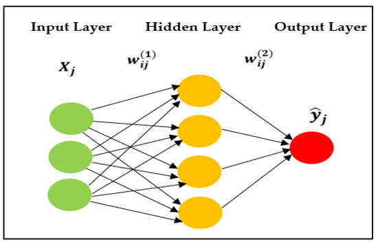
Figure 2.
A multilayer perceptron model with one hidden layer.
Here, the is the input to the neuron of the input layer, the is the weight of the link connecting neuron of the input layer to neuron of the hidden layer, is the bias associated with the neuron of the hidden layer, and is the activation function associated with the hidden layer. Then, the net output from neuron of the hidden layer is given by (see Equation (2)). is the weight of the link connecting neuron of the hidden layer to neuron of the output layer, is the bias associated with the neuron of the output layer, and is the activation function associated with the output layer. In this case, . The output of that neuron of the output layer (or, in our case, the final rainfall prediction at Rathnapura by MLP) will be [15]. Since the network is fully connected, each unit has its own bias, and there is a weight for every pair of units in two consecutive layers. Then, the MLP network computations can be written as:
2.2.3. Long Short-Term Memory (LSTM)
LSTM has four neural network layers interacting in a very special way. Its memory cell consists of a forget gate, input gate, and output gate [16].
As shown in Figure 3, the output of the last moment and current input value are fed into the forget gate to obtain the following output at the forget gate.
where , —weight at forget gate, —bias at forget gate, current input value, —output at previous moment. Then, the same previous output and current input value are inputted to the input gate, and the output value and candidate cell state at the input gate are calculated as below.
where , —weight at input gate, —bias at input gate, —weight at candidate input gate, —bias at candidate input gate. Update the current cell state using the following formulae.
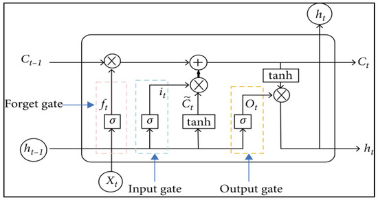
Figure 3.
LSTM structure diagram (Adapted with permission from Ref. [17]. 2020, Wenjie Lu et al.).
The and are then fed into output gate at time and obtain output at output gate as follows. Here, —weight at output gate and —bias at input gate.
Finally, the output of the LSTM was obtained using the current cell state and output at the output gate using the following formulae.
2.2.4. Convolutional Neural Network (CNN)
CNN is very popular for image processing and computer vision. It consists of three layers as seen in Figure 4. Convolution layer performs linear convolution operation, and the features of the data are extracted. Since the feature dimensions are very high, a pooling layer is added after the convolution layer. To make a final forecast, a fully connected (FC) layer (or dense layer) is added, and inputs to this layer are the flattened features resulted from convolutional and pooling layers [18,19].
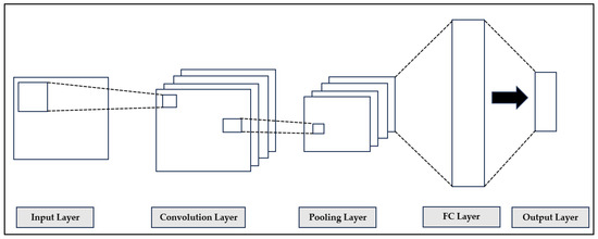
Figure 4.
The architecture of CNN.
2.2.5. Random Forest (RF)
RF is known as a supervised ensemble learning method. The method constructs a multitude of decision trees with controlled variation at the training phase. Then, using bagging, each tree in the ensemble is constructed (with sample with replacement) from training data. In the classification problem, each tree in ensemble is a base classifier to identify the class of the unlabeled observation. Through voting of each classifier for their predicted classes, the final class is obtained computing the majority votes [20,21].
2.2.6. Support Vector Machine (SVM)
SVM classifier finds a hyperplane to segregate the nodes for classification. The following optimization problem is solved when deriving the optimal hyperplane which separates two classes.
where is the class label, is the weights vector, is the input feature vector, is the transformation function, is the degree of misclassification corresponding to , is the regularization parameter and is the bias.
The optimal hyperplane (a maximum marginal hyperplane (MMH)) is learnt by training the samples using several kernel functions such as linear, radial basis function (rbf) and polynomial (poly) [22]. The Penalized SVM (PSVM or Cost-sensitive SVM) is a modification of SVM that weighs the margin proportional to the class importance which can be applied to an imbalanced dataset [23,24].
2.2.7. Naïve Bayes (NB)
The Naïve Bayes Algorithm is based on the Bayes Theorem of probability.
where, : The posterior probability of the class of interest given predictor, : The prior probability of the class of interest, : The probability of predictor given class C, and : The prior probability of predictor.
NB method calculates the probability of an observation belonging to a certain class. The Complement Naïve Bayes (CNB) method computes the probability of the observation belonging to all the classes. Thus, CNB is more suitable in dealing with imbalanced datasets [25].
2.2.8. Multinomial Logistic Regression (MLR)
Multinomial Logistic Regression is the generalization of Logistic regression which allows more than two categories of output variable. It also obtains maximum likelihood estimation to evaluate the probability of categorical membership [26]. The formula of MLR is as follows:
where is the probability of in class, is the probability of in class, is the intercept, is the vector of covariates for the class of the output variable , and is the input feature vector [27].
2.3. Imbalanced Learning
The data mining techniques will produce biased classification if the dataset is imbalanced [11]. Moreover, it can lead to a problem in ignoring the minority class entirely in the case where the predictions on the minority class are most important. This is a major issue found in rainfall forecasting. Certain methodologies can deal with the class imbalance of the data.
2.3.1. Cost—Sensitive Learning
This tactic uses penalized learning algorithms which give higher misclassification costs (or weights) for instances of the minority class and lower misclassification costs for the majority class [12,24].
2.3.2. Resampling Techniques
The resampling techniques are applied to obtain more balanced datasets. In this study, Synthetic Minority Oversampling Technique (SMOTE) which synthesizes new samples from the minority class was applied.
2.4. Model Evaluation
The metrics, Accuracy, Precision, Recall and F1-Score were used to evaluate the classification models, and the Spatial Kriging model results were evaluated using Mean Absolute Error (MAE), Root Mean Squared Error (RMSE), and R2 value.
Firstly, the cost-sensitive approach was followed in rainfall class prediction. Through the model evaluation results, the best set of models were chosen to apply the resampling technique. The final evaluation based on resampling was taken into consideration in selecting the best model for rainfall classification. Before applying the classification models, all the input variables were normalized. The machine learning and deep learning algorithms were run in Python.
3. Results and Discussion
As mentioned previously, initially the Spatial Kriging method was applied to find the daily rainfall prediction at Rathnapura gauging station.
The results shown in Table 1 indicate that the Spatial Kriging model fitted using the rainfall values of nearby stations cannot be solely used to explain the variation of the rainfall at target station, yet, they have an influence on the target station’s rainfall.

Table 1.
Performance of Spatial Kriging method.
Then, the previous day’s (t − 1) satellite image was modeled with the current day’s (t) rainfall occurrence in Rathnapura using the CNN model. The best model parameters obtained via 60 trials of training the models CNN, MLP and LSTM are presented in Table 2.
Table 2.
Parameter specification of CNN, MLP and LSTM models.
The CNN model showed 64.9% of Accuracy and Recall with 59.7% of Precision and 52.8% of F1-Score. The results also suggest the same conclusion produced by the Spatial Kriging method.
However, applying Spatial Kriging reduced the dimensions (number of input variables) of the final model. This method along with satellite images analysis are set to incorporate the spatial variation of the rainfall data to the final model.
The predictions obtained from the above two spatial models were incorporated as new predictor variables to the final dataset. Then, there were 23 predictor variables. The values of the past three days (t, t − 1, t − 2 on (2)) spatial correlation between nearby stations and target station to final model. t − 2) of each predictor variables were modeled with the next day (t + 1) actual rainfall class since through a preliminary data analysis we could identify that the past three days rainfall values have much impact on the next day (t + 1) rainfall occurrence.
To address the class imbalance, cost-sensitive models were applied. The entire data set was split as 80% for training and 20% for testing. For the training set, Repeated Stratified 5—Fold Cross Validation (which repeats the cross-validation procedure multiple times) was applied to further address the class imbalance problem. Table 3 and Table 4 show model performance.
Table 3.
The performance of cost-sensitive models in training sets.
Table 4.
The performance of cost-sensitive models in test set.
The training and testing performances indicate that cost-sensitive SVM, Random Forest, Multinomial Logistic Regression, and LSTM models have performed better in terms of metrics, especially precision, recall, and F1-score, which are more suitable in evaluating class-imbalanced problems [28]. The selected models depict more than 70% Accuracy, Precision, Recall, and F1-Score.
Then, for the selected models, the SMOTE resampling technique was applied. The performance was evaluated after refitting the balanced dataset using the selected best set of models. The following Table 5 and Table 6 illustrate the final performance results.
Table 5.
The performance of cost-sensitive resampled models in training set.
Table 6.
The performance of cost-sensitive resampled models in test set.
It can be observed that after two operations, the performance of all selected models has improved. Out of them, the Random Forest method gives the best and consistent performance in both the training set and in the final evaluation (in test set) of the selected models (nearly 88% of Accuracy, Precision, Recall, and F1-Score).
Overall, the study results indicate the importance of incorporating spatial variation of the rainfall data in predicting future events and highlight the effectiveness of step-wise imbalance learning to obtain consistent and more accurate predictions which could not be attained in some previous studies.
4. Conclusions
In this study, we proposed a novel ensemble spatiotemporal data mining approach to forecast rainfall occurrence at the Rathnapura gauging station. Spatial Kriging and a Deep Learning model (CNN) were employed to capture the spatial variation over the selected grid. The temporal variation of the rainfall data was brought to the model by modeling with the three past consecutive days’ values of the variables. Five cost-sensitive models were further improved to address the imbalanced problem found in rainfall classes through a resampling technique. The final performance summary emphasizes the outperformance of the cost-sensitive resampled Random Forest method (nearly 88% of accuracy, precision, recall, and F1-score) in forecasting future rainfall occurrences.
During the study, we found the complexity of working with high number of predictor variables. Therefore, our future studies are expected to enhance further by focusing on feature selection and application of dimension reduction prior to the model application. Collecting data for an extended period (e.g., 30 years) and selecting novel approaches will also be taken into consideration when dealing with highly imbalanced rainfall data.
Author Contributions
Conceptualization, C.T. and S.S.; methodology, S.S. and C.T.; software, S.S.; validation, S.S.; formal analysis, S.S.; investigation, C.T., M.M. and P.L.; resources, S.S.; data curation, S.S.; writing—original draft preparation, S.S.; writing—review and editing, C.T. and M.M.; visualization, S.S.; supervision, C.T., M.M. and P.L.; project administration, C.T.; funding acquisition, C.T. All authors have read and agreed to the published version of the manuscript.
Funding
This research was funded by the Research Grant of the University of Colombo, Sri Lanka, grant number AP/3/2019/CG/30.
Institutional Review Board Statement
Not applicable.
Informed Consent Statement
Not applicable.
Data Availability Statement
The data that support the findings of this study are available from the authors upon reasonable request.
Acknowledgments
The authors wish to acknowledge Irrigation Department of Sri Lanka for providing flood related data and the China Meteorological Administration National Satellite Meteorological Center (NSMC) for providing the satellite data for the study.
Conflicts of Interest
The authors declare no conflict of interest.
References
- Hussein, E.A.; Ghaziasgar, M.; Thron, C.; Vaccari, M.; Jafta, Y. Rainfall Prediction Using Machine Learning Models: Literature Survey. In Artificial Intelligence for Data Science in Theory and Practice; Studies in Computational, Intelligence; Alloghani, M., Thron, C., Subair, S., Eds.; Springer: Cham, Switzerland, 2022; Volume 1006. [Google Scholar] [CrossRef]
- Parmar, A.; Mistree, K.; Sompura, M. Machine Learning Techniques For Rainfall Prediction: A Review. In Proceedings of the 2017 International Conference on Innovations in information Embedded and Communication Systems (ICIIECS), Coimbatore, India, 17–18 March 2017. [Google Scholar]
- Sun, D.; Wu, J.; Huang, H.; Wang, R.; Liang, F.; Xinhua, H. Prediction of Short-Time Rainfall Based on Deep Learning. Math. Probl. Eng. 2021, 2021, 6664413. [Google Scholar] [CrossRef]
- Kannan, S.; Ghosh, S. Prediction of daily rainfall state in a river basin using statistical downscaling from GCM output. Stoch. Environ. Res. Risk Assess. 2010, 25, 457–474. [Google Scholar] [CrossRef]
- Ji, S.-Y.; Sharma, S.; Yu, B.; Jeong, D.H. Designing a rule-based hourly rainfall pre-diction model. In Proceedings of the 2012 IEEE 13th International Conference on Information Reuse & Integration (IRI), Las Vegas, NV, USA, 8–10 August 2012; Volume I. [Google Scholar] [CrossRef]
- Sharma, M. Comparative Study of rainfall forecasting models MA Sharma. JB Singh N. Y. Sci. J. 2011, 4, 115–120. [Google Scholar]
- Gao, L.; Wei, F.; Yan, Z.; Ma, J.; Xia, J. A Study of Objective Prediction for Summer Precipitation Patterns Over Eastern China Based on a Multinomial Logistic Regression Model. Atmosphere 2019, 10, 213. [Google Scholar] [CrossRef]
- Aguasca-Colomo, R.; Castellanos-Nieves, D.; Méndez, M. Comparative Analysis of Rainfall Prediction Models Using Machine Learning in Islands with Complex Orography: Tenerife Island. Appl. Sci. 2019, 9, 4931. [Google Scholar] [CrossRef]
- Zainudin, S.; Jasim, D.; Abu Bakar, A. Comparative Analysis of Data Mining Techniques for Malaysian Rainfall Prediction. Int. J. Adv. Sci. Eng. Inf. Technol. 2016, 6, 1148. [Google Scholar] [CrossRef]
- Singh, G.; Kumar, D. Hybrid Prediction Models for Rainfall Forecasting. In Proceedings of the 2019 9th Inter-national Conference on Cloud Computing, Data Science & Engineering (Confluence), Noida, India, 10–11 January 2019; pp. 392–396. [Google Scholar] [CrossRef]
- Oswal, N. Predicting rainfall using machine learning techniques. arXiv 2019, arXiv:1910.13827. [Google Scholar]
- Katrakazas, C.; Antoniou, C.; Yannis., G. Time Series Classification Using Imbalanced Learning for Real-Time Safety Assessment. In Proceedings of the Transportation Research Board 98th Annual Meeting, Washington, DC, USA, 13–17 January 2019. [Google Scholar]
- Cuenca, J.; Correa-Flórez, C.; Patino, D.; Vuelvas, J. Spatio-Temporal Kriging Based Economic Dispatch Problem Including Wind Uncertainty. Energies 2020, 13, 6419. [Google Scholar] [CrossRef]
- Abirami, S.P.; Chitra, P. Chapter Fourteen—Energy-efficient edge based real-time healthcare support system. Adv. Comput. 2020, 117, 339–368. [Google Scholar]
- Grosse, R. Lecture 5: Multilayer Perceptrons. 2018. Available online: https://www.cs.toronto.edu/~rgrosse/courses/csc321_2018/readings/L05%20Multilayer%20Perceptrons.pdf (accessed on 1 February 2023).
- Understanding LSTM Networks. Available online: https://colah.github.io/posts/2015-08-Understanding-LSTMs/ (accessed on 1 February 2023).
- Lu, W.; Li, J.; Li, Y.; Sun, A.; Wang, J. A CNN-LSTM-Based Model to Forecast Stock Prices. Complexity 2020, 2020, 6622927. [Google Scholar] [CrossRef]
- How Do Convolutional Layers Work in Deep Learning Neural Networks? Available online: https://machinelearningmastery.com/convolutional-layers-for-deep-learning-neural-networks/ (accessed on 1 February 2023).
- Torres, J.F.; Hadjout, D.; Sebaa, A.; Martínez-Álvarez, F.; Troncoso, A. Deep Learning for Time Series Forecasting: A Survey. Big Data. Feb. 2018, 2021, 3–21. [Google Scholar] [CrossRef]
- Goehry, B.; Yan, H.; Goude, Y.; Massart, P.; Poggi, J.M. Random Forests for Time Series. REVSTAT Stat. J. 2021. accepted. Available online: https://revstat.ine.pt/index.php/REVSTAT/article/view/400 (accessed on 1 February 2023).
- Fawagreh, K.; Gaber, M.; Elyan, E. Random Forests: From Early Developments to Re-cent Advancements. Syst. Sci. Control. Eng. 2014, 2, 602–609. [Google Scholar] [CrossRef]
- Yu, N.; Haskins, T. KNN, An Underestimated Model for Regional Rainfall Forecasting. arXiv 2021, arXiv:2103.15235. [Google Scholar]
- Cost-Sensitive SVM for Imbalanced Classification. Available online: https://machinelearningmastery.com/cost-sensitive-svm-for-imbalanced-classification/ (accessed on 2 February 2023).
- How to Handle Imbalanced Classes in Machine Learning. Available online: https://elitedatascience.com/imbalanced-classes (accessed on 2 February 2023).
- Complement Naive Bayes (CNB) Algorithm. Available online: https://www.geeksforgeeks.org/complement-naive-bayes-cnb-algorithm/ (accessed on 2 February 2023).
- Kwak, C.; Clayton-Matthews, A. Multinomial logistic regression. Nurs. Res. 2002, 51, 404–410. [Google Scholar] [CrossRef] [PubMed]
- Hashimoto, E.M.; Ortega, E.M.M.; Cordeiro, G.M.; Suzuki, A.K.; Kattan, M.W. The multinomial logistic regression model for predicting the discharge status after liver transplantation: Estimation and diagnostics analysis. J. Appl. Stat. 2019, 47, 2159–2177. [Google Scholar] [CrossRef] [PubMed]
- Andersson, M. Multi-Class Imbalanced Learning for Time Series Problem: An Industrial Case Study. Master’s Dissertation, Uppsala University, Uppsala, Sweden, 2020. Available online: http://urn.kb.se/resolve?urn=urn:nbn:se:uu:diva-412799 (accessed on 2 February 2023).


Disclaimer/Publisher’s Note: The statements, opinions and data contained in all publications are solely those of the individual author(s) and contributor(s) and not of MDPI and/or the editor(s). MDPI and/or the editor(s) disclaim responsibility for any injury to people or property resulting from any ideas, methods, instructions or products referred to in the content. |
© 2023 by the authors. Licensee MDPI, Basel, Switzerland. This article is an open access article distributed under the terms and conditions of the Creative Commons Attribution (CC BY) license (https://creativecommons.org/licenses/by/4.0/).